
The Relationship between River Flow Regimes and Climate Indices of ENSO and IOD on Code River, Southern Indonesia


1
Department of Environmental Engineering, Universitas Islam Indonesia, Yogyakarta 55584, Indonesia
2
Graduate School of Engineering, Gifu University, Gifu 5011193, Japan
3
River Basin Research Center, Gifu University, Gifu 5011193, Japan
*
Author to whom correspondence should be addressed.
Water 2021, 13(10), 1375; https://doi.org/10.3390/w13101375
Submission received: 6 April 2021
/
Revised: 30 April 2021
/
Accepted: 11 May 2021
/
Published: 14 May 2021
(This article belongs to the Section Hydrology)
Abstract
:Predicting the streamflow regimes using climate dynamics is important in water resource management. However, in Indonesia, there are few studies targeting climate indices and streamflow. A previous study found difficulty in developing a statistical prediction model for this relationship due to its non-linear nature. This study attempted to address that gap by applying multiple regression (MR) models using second- and third-order polynomial functions to show the non-linear relationship between climate and flow regime indices. First, a correlation analysis was performed to check the variable relationships. There was a good and significant correlation of El Niño Southern Oscillation (ENSO) with the flow regime indices. Secondly, MR models were developed with the same-time variables. The developed model showed that the Indian Ocean Dipole (IOD) had the effect of strongly increasing the high flow in La Niña phases. Finally, time-lagged MRs were developed aiming at forecasting. Lagged MR models with six-month leading climate indices demonstrated a relatively good correlation with the observed data (mostly R > 0.700) with moderate accuracy (root mean square error = 44–51%). It suggests that the forecasting of flow regime may be possible using ENSO and IOD indices.
1. Introduction
Understanding the pattern of streamflow dynamics is important in conserving an ecosystem and anticipating water disasters. The pattern of streamflow can be defined by the river flow regime. Flow regime is a term used by ecohydrologists to define five aspects of river flow: the magnitude, timing, frequency, duration, and rate of change [1,2]. Recently, the perspective of flow regime was suggested to be shifted toward the climate and ecological dynamics in the future [3]. In this context, studies to deepen the understanding and predictability of the flow regime based on climate are growing in importance.
Indonesian rainfall is known to be affected by the El Niño Southern Oscillation (ENSO). The ENSO is a periodical variation in sea surface temperatures over the Pacific Ocean, which consists of El Niño and La Niña phases. El Niño is known to correlate with less rainfall in Indonesia—causing drought over most parts of Indonesia—as opposed to La Niña, which increases the rainfall in Indonesia [4,5]. The influence of ENSO events was found to be well-correlated to rainfall in southern Indonesia [6,7].
Indonesian rainfall is also affected by another climate phenomenon—the Indian Ocean dipole (IOD) [8]. The IOD is a seasonal oscillation of sea surface temperatures in the Indian Ocean. The high activity of the IOD has been recognized to cause droughts in Indonesia [9]. A study in northwestern Java showed that IOD events affect the interannual rainfall variation in the dry season [10]. Furthermore, the rainfall in southern Sumatra and Java, facing the Indian Ocean, was negatively correlated with the IOD [7].
ENSO and IOD effects are also being studied for their direct influence on streamflows, especially for ENSO. An earlier study of the influence of ENSO on streamflows in 1993 found that there was a coherent and significant streamflow response to ENSO in four regions of the United States [11]. The effect of ENSO on streamflows has been studied in many regions around the world [12,13,14,15].
In Indonesia, there was a study of the effects of ENSO and IOD on the streamflow in Citarum River, West Java [16]. The study found that the extreme high streamflow events were associated with La Niña and negative IOD, while the extreme low streamflow events were associated with positive IOD and El Niño. However, the authors of [16] acknowledged the difficulty in developing a statistical prediction model of the relationship due to various climate phenomena. The authors of [16] claimed that the relationship of ENSO and IOD on streamflow becomes non-linear in some seasons, and thus they focused the discussion only on the peak of the IOD event with a correlation analysis.
The relationship between ENSO and IOD also has been questioned for their independency to each other. While many studies have reported that the IOD is statistically independent to ENSO (e.g., [9,17,18,19], some studies argued that the ENSO and IOD are not totally independent (e.g., [20,21,22]).
In this study, we attempted to investigate the non-linear relationship of ENSO and IOD on streamflow by applying multiple polynomial regression analysis. We aimed to demonstrate the predictability of streamflow regimes using ENSO and IOD in Code River, southern Java Island, Indonesia (Figure 1). The study mainly consisted of three parts. First, we investigated the relationship of ENSO and IOD with streamflow by correlation analysis. Secondly, multiple polynomial regression models using ENSO and IOD indices as predictors were developed with consideration of the average duration. Finally, the forecasting ability of a time-lagged regression model was investigated. The streamflow forecast using climate indices will be beneficial for water resource management.
2. Study Area
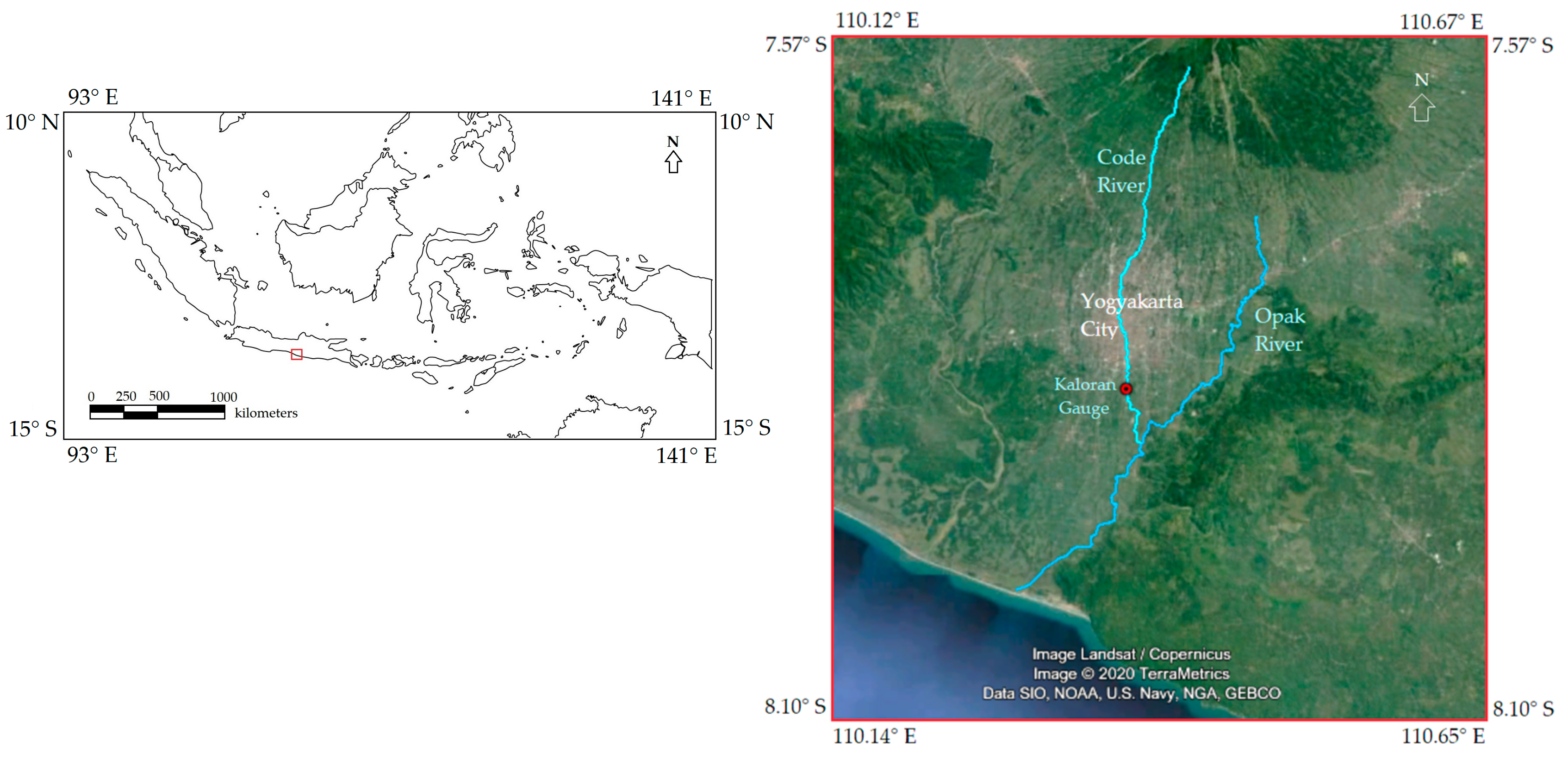
The Special Region of Yogyakarta is a small Indonesian province located in the southern central region of Java Island, occupying an area of 3179 km2. One of the main rivers in the province is Opak River. Many streams of Opak River tributaries cross in the center of the province in Yogyakarta City. One of the tributaries is Code River, a well-known stream, which often represents Yogyakarta City. Code River basin occupies an area of approximately 40 km2. Code River joins Opak River after traveling south for 41 km from its spring on Mount Merapi, north of Yogyakarta (Figure 1). As the stream is situated in a strategic location, Code River holds not only cultural value but also aesthetic value and tourism potential [23].
Based on the Köppen climate type, the Yogyakarta region typically has a tropical savanna (Aw) climate type. Sometimes, this region has a tropical monsoon (Am) climate type. The region has dry months from May to October (MJJASO)—with August as the driest—and wet months from November to April (NDJFMA)—with January or February as the wettest. The annual rainfall varies between 400 to 3600 mm. The average temperature varies from 22 °C in the upstream area to 27 °C in the downstream area. The lowest temperatures occur in the dry months (June to August). The dry months have lower temperatures compared with the wet months owing to the cold wind from the southern hemisphere (Australia) winter [24].
3. Data and Methods
3.1. Data
The streamflow data used in this study were from the gauge station Kaloran in the downstream part of Code River (Figure 1). The streamflow dataset was obtained from the Indonesian Ministry of Public Works and Housing. The daily streamflow data of Kaloran station is available for 21 years, covering 1994 to 2018. The river flow regime parameters used in this study are the average flow, high flow, and low flow as defined by the flow duration curve. The average flow was Q50 (50% percentile flow), the high flow was Q10 (10% percentile flow), and the low flow was Q90 (90% percentile flow). The high flow index is important for flood prevention, while the low flow index is useful for drought anticipation and environmental flow setting.
The climate variables used in this study are the Southern Oscillation Index (SOI) as the ENSO index and Dipole Mode Index (DMI) as the IOD index. The DMI is the commonly used index for IOD, and it is easily obtainable. The SOI was chosen as an easily defined traditional ENSO index and it is frequently used by researchers to show the relationship between ENSO and precipitation (e.g., [25,26]). The ENSO year annual variations and rainfall patterns in Indonesia were in high coherence, as shown by the SOI in a long-series dataset (1885–1983) [25]. The measure of SOI is based on the difference in sea level pressures between Darwin and Tahiti [27]. In contrast, the other ENSO indices were mostly based on the sea surface temperature anomalies in the tropical Pacific Ocean, such as NINO 3.4. The NINO 3.4 was identified as the most representative index for ENSO since the publication in 1997 [28] and was frequently used in recent studies (e.g., [19,29,30]). SOI and NINO 3.4 were well-correlated and not statistically different in most of the seasons [28]. Our calculations also indicated that SOI gave a slightly better correlation than NINO 3.4 in a longer duration average (not shown). Hence, the traditional SOI is used in this study. The SOI (standardized) and DMI data were obtained from the National Oceanic and Atmospheric Administration (NOAA) of the USA.
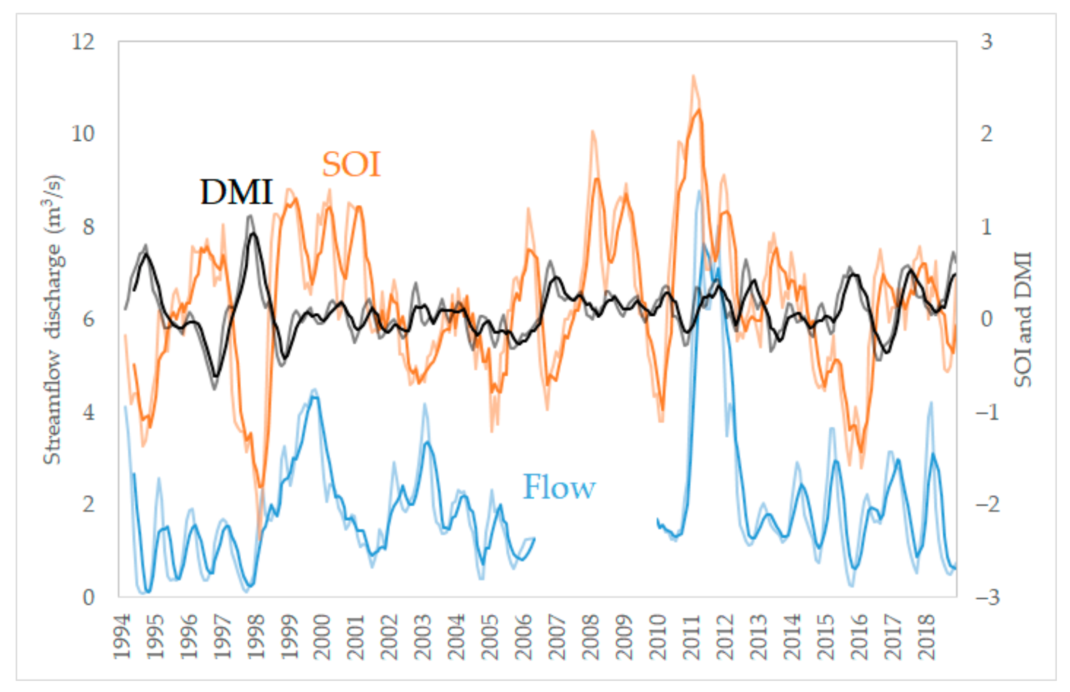
The time series of the 3- and 6-month averaged data of streamflow, SOI, and DMI are shown in Figure 2. The missing data of streamflow from the period 2006–2009 are dominated by La Niña (high SOI) events in the wet seasons of 2008 and 2009. The strong La Niña events in 2011 can cover the information of strong La Niña events on the analysis. The strong El Niño (low SOI) events captured in 1998/1999 and 2015/2016 were two of the three super El Niño events identified since 1980 [29].
3.2. Methods
The Pearson correlation was used to find the correlation coefficient R. The datasets used for the analysis were monthly data. While the climate indices were already in the monthly dataset, the monthly flow regime indices datasets were obtained by extracting the Q50, Q10, and Q90 from the 1-month daily data. The significance of the correlation was evaluated using a two-tailed t-test at the 95% confidence level.
Regression models were developed using SOI and DMI as predictors to predict the average (Q50), high (Q10), and low (Q90) flow indices. We found that the correlation coefficient between monthly SOI and DMI is −0.316, which is statistically insignificant. However, the deviation from the dependent part has importance. Therefore, we used both SOI and DMI on the prediction of streamflow using multiple regression models. Multiple regression models were developed using first-, second-, and third-order polynomial functions. The calculation of regression model parameters was performed at a 95% confidence level.
The estimated value of the regression models was then calculated by taking the model term coefficients to the equation of the regression models as shown in Equations (1)–(3). The accuracy of the regression models was evaluated by the estimated–observed correlation coefficient and the standard error of the regression models. The calculation for the standard error of estimation used the root mean square error (RMSE) following Equation (4) [31] and is displayed as a percentage to the average of the observed values.
The model equation of the first-order polynomial regression with two predictors:
y = β0 + β1 × 1 + β2x2 + ε.
The model equation of the second-order polynomial regression with two predictors:
y = β0 + β1x1 + β2x2 + β3x12 + β4x22 + β5x1x2 + ε.
The model equation of the third-order polynomial regression with two predictors:
with:
y = β0 + β1x1 + β2x2 + β3x12 + β4x22 + β5x1x2 + β6x13 + β7x23 + β8x12x2 + β9x1x22 + ε
y = flow regime index (Q50, Q10, Q90);
x1 = SOI;
x2 = DMI;
β = coefficient of model term; and
ε = model error.
with:
y = observed values;
y’ = estimated values;
N = number of observations;
k = number of parameters to be estimated (the number of β, except the intercept); and
notes the summation for the monthly set of the x1, x2, and y.
4. Results
4.1. Correlation Analysis
The coefficients of the correlation between the observed flow regime indices and climate indices (SOI and DMI) in the monthly datasets are shown in Table 1. SOI (ENSO) had a distinctively higher correlation with the flow regime indices than the DMI (IOD). The coefficients of the correlation of the climate indices with the flow regime indices were between 0.330 to 0.347 for SOI and −0.031 to −0.099 for DMI. Although the SOI correlations are at a lower level, they are statistically significant. The correlation of DMI to the streamflow in this study is negligible due to its near-zero correlation coefficients. Previous studies in northwestern Java showed that rainfall had a negative correlation with IOD [10] and that most low flow events in rivers were linked with a positive IOD [16]. These different results may be caused by different timescales used by the studies. It is discussed further in Section 5.1.
The correlation coefficients on 3- and 6-month moving averaged datasets were also calculated to investigate the temporal effect. The 3- and 6-month moving average time series are also shown in Figure 2. Six months was the longest averaging period to show the Indonesian biannual seasons. For the SOI, the 6-month moving average had a higher correlation than did the 3-month moving average and the original dataset. The 6-month moving average increased the correlation coefficient from the original dataset by 0.167, 0.136, and 0.157 for Q50, Q10, and Q90, respectively. These results signal that the ENSO effect has a longer timescale than 1 month and that the peak is at the 6-month scale. On the other hand, the moving average datasets of DMI did not show a noticeable change from the original datasets.
The correlation coefficient becomes higher at the longer timescale of the moving average. It is because the moving average eliminated the variations which are shorter than the averaging period. This tendency may be related to the elimination of variation under a 3- or 6-month timescale; for example, Madden–Julian Oscillation (MJO). The active phase of MJO, which lasts about 1 or 2 months [32], has been known to increase the extreme precipitation events over western and central Indonesia [33]. We eliminated this kind of noise because this study focused on the ENSO and IOD, which are in a longer timescale variation.
The effect of ENSO on the flow regime was clearly more dominant than the effect of DMI in Code River (Table 1). Based on the two-tailed t-test, the correlations of SOI to the flow regime indices were all significant, as opposed to the DMI correlations to the flow regime indices, which were all not significant. With low and insignificant correlation values, IOD had no association with the observed streamflow of Code River. ENSO, on the other hand, had a positive association with the streamflow—and was the highest in a 6-month timescale. This effect of ENSO was essentially the same with Q50, Q10, and Q90.
The moving average may be considered to reduce the degree of freedom of the data and may change the result of statistical analysis. Therefore, we checked the worst case by calculating the correlation coefficient using one datum for each averaging period. For the 3-month (6-month) moving average, it was one datum every 3 (6) months, making a total number of data used in each analysis become one-third (one-sixth) of the original moving average datasets had. The results are similar to the values in Table 1. For example, the correlation coefficient of Q50 in the 3- and 6-month moving average by this calculation are 0.440 and 0.516, respectively. The status of the significancy also did not change.
4.2. Multiple Regression Analysis
Equations (1)–(3) were used to develop multiple polynomial regression (MR) models to estimate the Q50, Q10, and Q90 using SOI and DMI as predictors, with the original dataset and 3- and 6-month moving average datasets. The regression models were evaluated by correlation coefficients (R) between the estimated and the observed flow regime (Q50, Q10, and Q90), root mean square error (RMSE, Equation (3), and the adjusted coefficient of determination (R2).
Higher R values between the estimated and observed flow regimes were identified on higher order regressions and longer timescales (Table 2). The highest correlation (R = 0.746) was achieved by the third-order MR for Q50 in the 6-month moving average timescale. The higher order MRs and a longer timescale of moving average were identified as having a lower RMSE and a higher adjusted R2 (Figure 3). The results suggest that the best model’s skill was achieved by the 6-month moving average dataset with third-order MR. Due to the much lower model’s skill achieved by first-order MR, from now on the first-order MR will be omitted from the analysis.
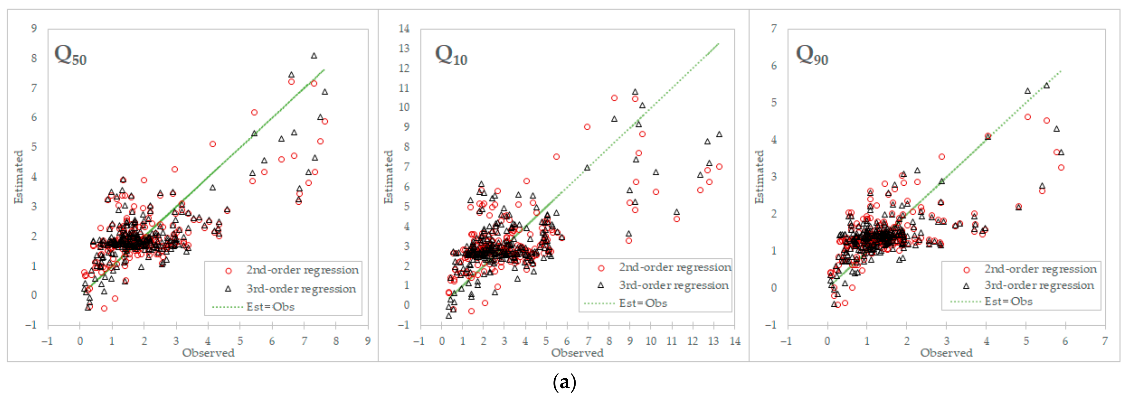
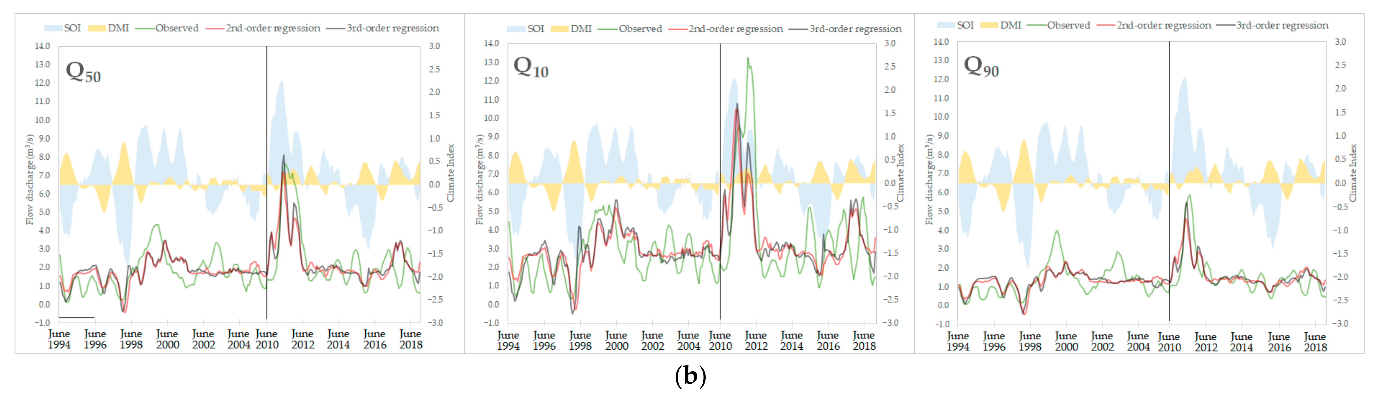
Figure 4 shows the estimated results of the 6-month moving average MR models in scatterplots and time series graphs. The scatterplot of the estimated versus observed values in Figure 4 shows that Q50 had the most accurate estimates and that the Q10 had the least accurate estimates. For all flow indices, both second- and third-order MR models had a tendency to underestimate in higher flows. On all flow indices, the third-order MR estimate tended to have a higher value compared with the second-order estimate. The MR models shown in time series (Figure 4) showed that the models had the highest accuracy, mostly in the extreme values, corresponding to strong (positive and negative) SOI values, such as in late 1994, mid-1998, early 2011, and late 2015.
4.3. Lagged Multiple Regression Analysis
The objective of MR analysis with variables at the same period was to investigate the tendencies of the relationships and cannot be used for forecasting the future without dynamical model prediction. A lagged MR with different periods of response and predictor variables should be used for forecasting the future of the response variables. The climate indices in this study may be able to forecast streamflow in the future with a few months lag applied in the MR. This possibility was attempted in this study through analyzing the MR with the climate indices dataset of 6 months before the streamflow dataset.
The MR with the same period variables (the MR used in Section 4.2) is labeled by lag0 and the MR with 6-month lagged variables is labeled by lag6. The lag0 regression result is provided in Section 4.2 and shows that the 6-month moving average was the best timescale to reduce variation noises and achieve the highest model skill (highest correlation with the observed flow, lowest standard error, and highest coefficient of determination). Hence, in this lagged MR, we used only the 6-month moving average dataset with second- and third-order MR. Additionally, the lag6 MR did not temporally overlap with the use of the 6-month moving average dataset. The model evaluations are shown in Table 3 and Figure 5.
Based on the correlation coefficient (R) of the estimated and observed values, lag6 performed well with a higher R compared with lag0. The third-order regressions had a higher correlation to the observed values than the second-order regressions. However, both orders showed similar patterns (Figure 5). The evaluation of the RMSE and adjusted R2 showed that the lag6 regressions had a lower error and higher R2 compared with lag0, but not by much. This indicates that lagged-time regressions had a slightly better accuracy over the same-time regressions in predicting the flow regimes using SOI and DMI. With these evaluation results, the lag6 MR is able to make forecasts regarding streamflow.
5. Discussion
5.1. IOD Climate Effects
The correlation analysis showed that SOI was a prominent indicator of streamflow while DMI was not. Despite its low and insignificant correlation in this study, DMI has been acknowledged for its effect on rainfall (and thus streamflow) in Indonesia [7,9,10]. A previous study in West Java clearly identified a positive IOD (with DMI) in the low flow period [16]. The timescale of the previous study was 3 months, focusing on the September–November (SON) period. In contrast, this study considered all months. The correlation analysis results (Section 4.1) captured the correlation of the ENSO-streamflow but could not capture the correlation of the IOD-streamflow.
Despite the low correlation of IOD to the flow regime indices (Section 4.1), the time series of the observed and estimated flows showed that the period of high positive IOD mostly appeared in events of extremely low flow, such as in the year 1994 (Figure 1 and Figure 5). This agrees with the previous study, which concluded that positive IOD was associated with low flow periods. Considering that the regression models in this study presented relatively good evaluations, IOD can be confirmed to modulate the ENSO–streamflow relationship.
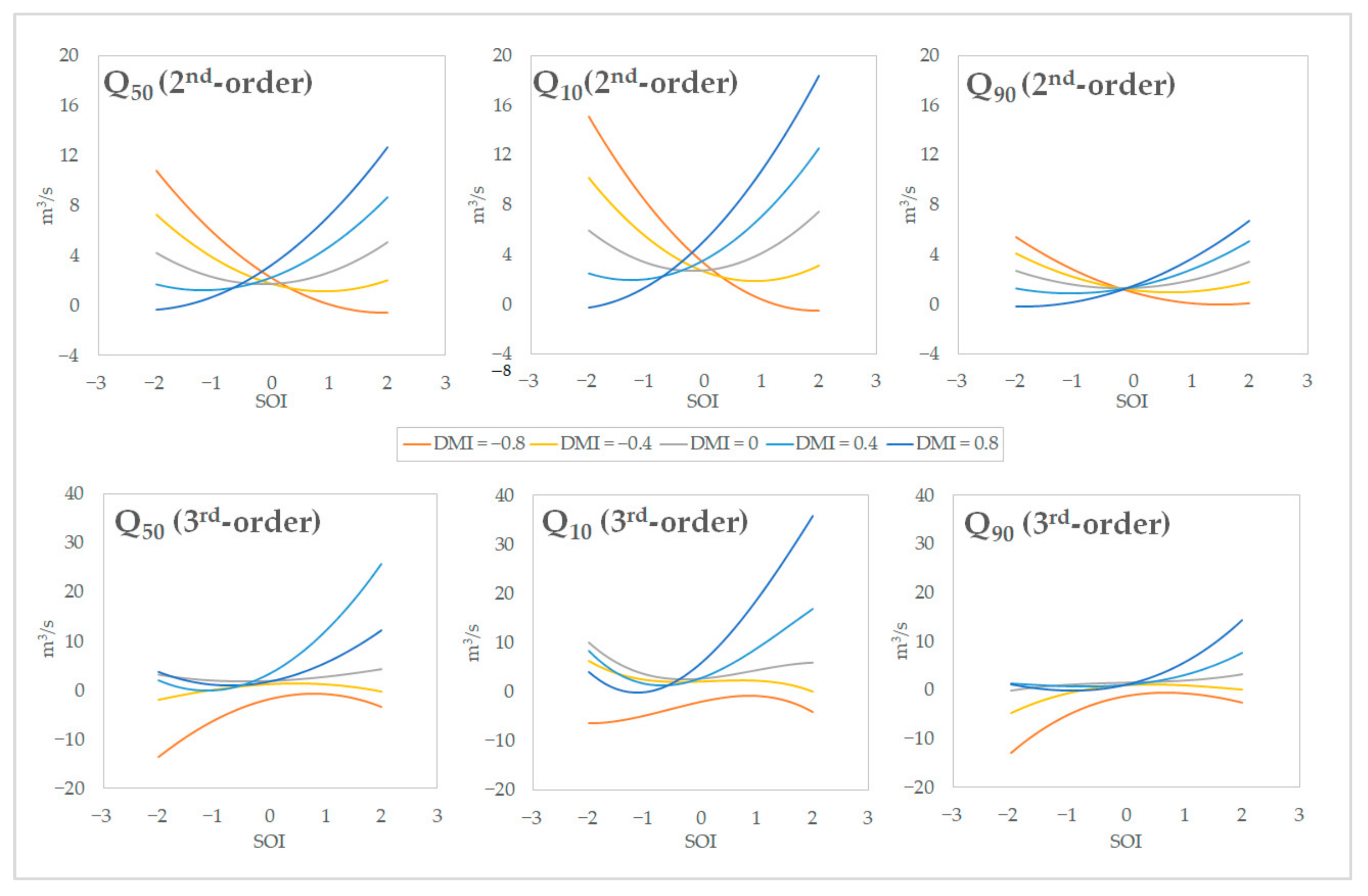
To further investigate the IOD contribution to the ENSO–streamflow relationship in the model we developed, we applied the second- and third-order regression models (6-month moving average) on varied dummy values of SOI and DMI. The range of SOI (DMI) values in the 6-month moving average dataset was −1.80 to 2.27 (−0.61 to 0.93), and thus the SOI (DMI) variation in this simulation was set from −2 to 2 (−0.8 to 0.8). The correlation of SOI–streamflow is already known to be positive; thus, a higher SOI should produce higher streamflow. In this case, we tested whether positive DMI (pDMI) and negative DMI (nDMI) changed the tendency of the positive relationship.
The behavior of MR functions is depicted by simulation using the dummy data in Figure 6. The simulations showed that in a higher positive SOI (pSOI), a higher pDMI produced a more significant increase in the streamflow, and a lower nDMI produced a relatively constant decrease in the streamflow. The second-order MR produced more physically appropriate estimates than the third-order MR, which allowed the estimate values to be below zero, especially on a negative SOI (nSOI). It is due to the lack of variance of nSOI-nDMI combination in the dataset for developing the regression models.
In this dummy simulation, the effect of DMI on the SOI–streamflow relationship in this simulation was more apparent at a higher flow to strongly increase the flow in positive SOI events. This modulation of SOI dependency due to the DMI cannot be expressed in linear (first-order) MR. This is due to the crossing terms containing both SOI and DMI included in the second- or third-order MR equations are necessary to express this modulation.
5.2. Flow Regimes Forecasting
The flow regime index Q50 can be beneficially used for the general purpose of water resource management, while Q10 and Q90 can be used for anticipating flood and drought events, respectively. Six months in advance is a good period for forecasting the flow regime in the sense of water resource management. This provides sufficient time for counteracting the impact of the flow regime behavior in the future. The evaluation of the 6-month lagged multiple regression models in this study showed a good correlation and moderate accuracy (Table 3). This indicates that the current last 6-month average of SOI and DMI would be able to predict the Q50, Q10, and Q90 6 months in the future using the regression model coefficients developed in this study (Table 4), with some notes on the accuracy.
Simple and usable models are important for practical uses, such as forecasting. The goal in developing multiple regression equations is to include meaningful variables that explain most of the data variability [34]. In general, the second-order MR is recommended by considering its model evaluation which was good enough and not far behind the third-order MR (Table 3). Furthermore, a lower order polynomial MR can keep the model equation simple and may prevent extreme results in the case of inputs outside the considered range.
The Q50 MR models had similar accuracy in second- and third-order MR (Figure 5), indicating that both regression orders can be used to forecast Q50 with a tendency to underestimate. The only noticeable difference between the two MR orders was in the combination event of strong negative IOD (less than −0.5) and strong positive ENSO (greater than 0.5). In such an event, which was captured only once in this study (in 1997), the third-order MR estimated an immediate reduced flow, while the second-order MR did not (Figure 5, bottom row). For the general purpose of river flow information, a simpler equation with second-order regression may be better.
The Q10 MR models have the least accuracy among the three flow indices (Figure 5). The most accurate estimation of the model was only found in two events with a combination of positive SOI and positive DMI, in 2011–2012 and 2018. Although the accuracy of both was similar, the third-order MR was better than the second-order regression in forecasting Q10. This is because the third-order MR tended to produce a higher estimate than the second-order MR (especially in the event of positive SOI and DMI). A higher estimation of high flow is usually favored to set a safety margin in the event of floods.
The Q90 MR models had better accuracy in the third-order MR than in the second-order MR (Figure 5). The MR models of Q90 had almost equal numbers in producing underestimated and overestimated values. However, the underestimated (overestimated) values tended to be in the higher (lower) level of Q90, while an underestimation is more favorable for anticipating drought and conserving ecosystems in rivers.
5.3. Model Validation
The relationships among variables found in this study are expected to be useful for predicting streamflow using the climate indices. The regression equations in this study (Table 4) can be used for forecasting after model validation is applied to them. However, we could not conduct model validation due to a lack of enough data. The streamflow data we obtained only covered 21 years, which included only four or five ENSO cycles. We need all 21 years of data to capture the variations of ENSO and IOD. We concluded that the IOD modulates the ENSO–streamflow relationship. Hence, with more ENSO and IOD data for at least two additional ENSO cycle periods, we would be able to capture the modulation in our models and make a model validation.
6. Conclusions
We developed multiple regression (MR) models to predict the flow regimes of Code River using the ENSO and IOD indices with second- and third-order polynomial functions. First, the relationship of the SOI (ENSO) and DMI (IOD) to the Code River streamflow was checked. Good and significant correlations of SOI to the flow regime indices were found in the 6-month moving average dataset. However, the use of monthly data in this study could not capture the effect of IOD in a simple correlation analysis.
Despite the insignificant low DMI correlation to the flow regime indices, the observed and estimated values in this study mostly agreed with a previous study in Citarum River, in that the extreme low flows appeared in strong positive IOD periods. Considering the relatively good model evaluation obtained by the MR models in this study, in further investigation, the IOD was confirmed to modulate the ENSO–streamflow relationship. This effect could be captured by second- and third-order polynomial MRs. The effect of IOD on the streamflow was identified to greatly increase the higher flows (of Q50 and Q10) in the positive ENSO phases.
In the MR analysis, the 6-month moving average was identified as the highest correlated timescale. We also identified that the third-order regression was a better model skill compared with the second-order regression. However, the difference between their estimation results was not significant. Therefore, both regression orders can be used to make a prediction. A time-lagged MR analysis was conducted using the 6-month moving average dataset and the two regression orders. We found that 6-month lagged (lag6) MR were better in explaining more variability of the flow regime compared with the same-time (lag0) MR. The lag6 MR model showed a relatively good evaluation with moderate accuracy: most R values with the observed data were over 0.700, 44–51% RMSE, and 0.470–0.590 adjusted R2.
Flow regime forecasting using 6-month lagged (lag6) multiple polynomial regression was possible with some caution regarding the model’s accuracy. Q50 was found to have the most stable and accurate estimates and thus, it is recommended for use with second-order MR for forecasting. Q10 and Q90 demonstrated lower model accuracy, and we recommend using third-order MR for forecasting. It is beneficial for water resource managers to be able to forecast the flow regime indices in the next 6 months using climate indices.
The lag6 MR model is expected to be useful for streamflow forecasting after a proper model validation in the future. In this study, the model validation could not be done due to a lack of data, making the validation work for the future. This study was, nonetheless, able to demonstrate non-linear climate–streamflow relationships and streamflow predictability with the climate indices using multiple polynomial regressions.
Author Contributions
Conceptualization, A.R.N. and I.T.; methodology, I.T.; software, A.R.N.; validation, A.R.N. and I.T.; formal analysis, A.R.N.; investigation, A.R.N.; resources, I.T.; data curation, A.R.N.; writing—original draft preparation, A.R.N.; writing—review and editing, I.T. and M.H.; visualization, A.R.N.; supervision, I.T.; project administration, A.R.N.; funding acquisition, A.R.N. and I.T. All authors have read and agreed to the published version of the manuscript.
Funding
This research received no external funding.
Institutional Review Board Statement
Not applicable.
Informed Consent Statement
Not applicable.
Data Availability Statement
SOI data can be found here: https://www.cpc.ncep.noaa.gov/data/indices/soi (accessed on 12 May 2021). DMI data can be found here: https://psl.noaa.gov/gcos_wgsp/Timeseries/Data/dmi.had.long.data (accessed on 12 May 2021). The Code River streamflow data are available on request from the Indonesian Ministry of Public Works, Direktorat Bina Teknik Sumber Daya Air ([email protected]).
Conflicts of Interest
The authors declare no conflict of interest.
References
- Richter, B.D.; Baumgartner, J.V.; Powell, J.; Braun, D.P. A Method for Assessing Hydrologic Alteration within Ecosystems. Conserv. Biol. 1996, 10, 1163–1174. [Google Scholar] [CrossRef] [Green Version]
- Poff, N.L.; Allan, J.D.; Bain, M.B.; Karr, J.R.; Prestegaard, K.L.; Richter, B.D.; Sparks, R.E.; Stromberg, J.C. The Natural Flow Regime. Bioscience 1997, 47, 769–784. [Google Scholar] [CrossRef]
- Poff, N.L. Beyond the natural flow regime? Broadening the hydro-ecological foundation to meet environmental flows challenges in a non-stationary world. Freshw. Biol. 2018, 63, 1011–1021. [Google Scholar] [CrossRef]
- Ropelewski, C.F.; Halpert, M.S. Global and Regional Scale Precipitation Patterns Associated with the El Niño/Southern Oscillation. Mon. Weather Rev. 1987, 115, 1606–1626. [Google Scholar] [CrossRef] [Green Version]
- Hendon, H.H. Indonesian rainfall variability: Impacts of ENSO and local air-sea interaction. J. Clim. 2003, 16, 1775–1790. [Google Scholar] [CrossRef]
- Aldrian, E.; Susanto, R.D. Identification of three dominant rainfall regions within Indonesia and their relationship to sea surface temperature. Int. J. Climatol. 2003, 23, 1435–1452. [Google Scholar] [CrossRef]
- Lee, H.S. General Rainfall Patterns in Indonesia and the Potential Impacts of Local Seas on Rainfall Intensity. Water 2015, 7, 1751–1768. [Google Scholar] [CrossRef]
- Aldrian, E.; Dümenil Gates, L.; Widodo, F.H. Seasonal variability of Indonesian rainfall in ECHAM4 simulations and in the reanalyses: The role of ENSO. Theor. Appl. Climatol. 2007, 87, 41–59. [Google Scholar] [CrossRef] [Green Version]
- Saji, N.; Goswami, B.; Vinayachandran, P.; Yamagata, T. A dipole mode in the Tropical Ocean. Nature 1999, 401, 360–363. [Google Scholar] [CrossRef] [PubMed]
- Jun-Ichi, H.; Mori, S.; Kubota, H.; Yamanaka, M.D.; Haryoko, U.; Lestari, S.; Sulistyowati, R.; Syamsudin, F. Interannual rainfall variability over northwestern Jawa and its relation to the Indian Ocean Dipole and El Niño-Southern Oscillation events. Sci. Online Lett. Atmos. 2012, 8, 69–72. [Google Scholar] [CrossRef] [Green Version]
- Kahya, E.; Dracup, J.A. U.S. streamflow patterns in relation to the El Niño/Southern Oscillation. Water Resour. Res. 1993, 29, 2491–2503. [Google Scholar] [CrossRef]
- Cardoso, A.O.; Silva Dias, P.L. The relationship between ENSO and Paraná River flow. Adv. Geosci. 2006, 6, 189–193. [Google Scholar] [CrossRef] [Green Version]
- Cluis, D.; Laberge, C. Analysis of the El Niño Effect on the Discharge of Selected Rivers in the Asia-Pacific Region. Water Int. 2002, 27, 279–293. [Google Scholar] [CrossRef]
- Zhang, Q.; Xu, C.Y.; Jiang, T.; Wu, Y. Possible influence of ENSO on annual maximum streamflow of the Yangtze River, China. J. Hydrol. 2007, 333, 265–274. [Google Scholar] [CrossRef]
- Mohsenipour, M.; Shahid, S.; Nazemosadat, M.J. Effects of El Nino Southern Oscillation on the Discharge of Kor River in Iran. Adv. Meteorol. 2013, 2013. [Google Scholar] [CrossRef]
- Sahu, N.; Behera, S.K.; Yamashiki, Y.; Takara, K.; Yamagata, T. IOD and ENSO impacts on the extreme stream-flows of Citarum river in Indonesia. Clim. Dyn. 2012, 39, 1673–1680. [Google Scholar] [CrossRef]
- Ashok, K.; Guan, Z.; Yamagata, T. Influence of the Indian Ocean Dipole on the Australian winter rainfall. Geophys. Res. Lett. 2003, 30, 3–6. [Google Scholar] [CrossRef]
- Behera, S.K.; Luo, J.J.; Masson, S.; Rao, S.A.; Sakuma, H.; Yamagata, T. A CGCM study on the interaction between IOD and ENSO. J. Clim. 2006, 19, 1688–1705. [Google Scholar] [CrossRef]
- Hendrawan, I.G.; Asai, K.; Triwahyuni, A.; Lestari, D.V. The interanual rainfall variability in Indonesia corresponding to El Niño Southern Oscillation and Indian Ocean Dipole. Acta Oceanol. Sin. 2019, 38, 57–66. [Google Scholar] [CrossRef]
- Xie, S.P.; Annamalai, H.; Schott, F.A.; McCreary, J.P. Structure and mechanisms of South Indian Ocean climate variability. J. Clim. 2002, 15, 864–878. [Google Scholar] [CrossRef] [Green Version]
- Kajtar, J.B.; Santoso, A.; England, M.H.; Cai, W. Tropical climate variability: Interactions across the Pacific, Indian, and Atlantic Oceans. Clim. Dyn. 2017, 48, 2173–2190. [Google Scholar] [CrossRef] [Green Version]
- Rao, J.; Garfinkel, C.I.; White, I.P.; Schwartz, C. The Southern Hemisphere Minor Sudden Stratospheric Warming in September 2019 and its Predictions in S2S Models. J. Geophys. Res. Atmos. 2020, 125, 1–19. [Google Scholar] [CrossRef]
- Soemardiono, B.; Gusma, A.F. The Development of Code River Area in Yogyakarta as a Sustainable Urban Landscape Asset acknowledging Local Traditional Knowledge. Int. Rev. Spat. Plan. Sustain. Dev. 2014, 2, 4–18. [Google Scholar] [CrossRef] [Green Version]
- Smith, P.J.; Krishnamurti, T.N.; Gentili, J. Malaysian-Australian Monsoon. Encyclopedia Britannica. Available online: https://www.britannica.com/science/Malaysian-Australian-monsoon (accessed on 12 May 2021).
- Ropelewski, C.F.; Halpert, M.S. Precipitation Patterns Associated with the High Index Phase of the Southern Oscillation. J. Clim. 1989, 2, 268–284. [Google Scholar] [CrossRef] [Green Version]
- Hamada, J.I.; Yamanaka, M.D.; Matsumoto, J.; Fukao, S.; Winarso, P.A.; Sribimawati, T. Spatial and temporal variations of the rainy season over Indonesia and their link to ENSO. J. Meteorol. Soc. Jpn. 2002, 80, 285–310. [Google Scholar] [CrossRef] [Green Version]
- Trenberth, K.E. Signal Versus Noise in the Southern Oscillation. Mon. Weather Rev. 1984, 112, 326–332. [Google Scholar] [CrossRef] [Green Version]
- Bamston, A.G.; Chelliah, M.; Goldenberg, S.B. Documentation of a Highly ENSO-Related SST Region in the Equatorial Pacific: Research Note. Atmos. Ocean 1997, 35, 367–383. [Google Scholar] [CrossRef]
- Rao, J.; Ren, R. Parallel comparison of the 1982/83, 1997/98 and 2015/16 super El Niños and their effects on the extratropical stratosphere. Adv. Atmos. Sci. 2017, 34, 1121–1133. [Google Scholar] [CrossRef]
- Qian, H.; Xu, S.B. Prediction of Autumn Precipitation over the Middle and Lower Reaches of the Yangtze River Basin based on Climate Indices. Climate 2020, 8, 53. [Google Scholar] [CrossRef] [Green Version]
- Pardoe, I. Applied Regression Modelling; Wiley: Hoboken, NJ, USA, 2012; ISBN 978-1-1180-9728-1. [Google Scholar]
- Madden, R.A.; Julian, P.R. Detection of a 40–50 Day Oscillation in the Zonal Wind in the Tropical Pacific. J. Atmos. Sci. 1971, 28, 702–708. [Google Scholar] [CrossRef]
- Muhammad, F.R.; Lubis, S.W.; Setiawan, S. Impacts of the Madden–Julian oscillation on precipitation extremes in Indonesia. Int. J. Climatol. 2020, 1970–1984. [Google Scholar] [CrossRef]
- Gordon, N.D.; McMahon, T.A.; Finlayson, B.L.; Gippel, C.J.; Nathan, R.J. Stream Hydrology: An Introduction for Ecologists, 2nd ed.; John Wiley & Sons: Chichester, UK, 2004; p. 368. ISBN 0-470-84357-8. [Google Scholar]
Figure 1.
Code River location in southern Indonesia. The small red box in the left figure (map of Indonesia) shows the location of the right figure (satellite image of Yogyakarta Region).
Figure 1.
Code River location in southern Indonesia. The small red box in the left figure (map of Indonesia) shows the location of the right figure (satellite image of Yogyakarta Region).

Figure 2.
Time series of Code River downstream flow, Southern Oscillation Index (SOI), and Dipole Mode Index (DMI), with a 6-month moving average and 3-month moving average (light color). The streamflow data of the years 2006 to 2009 are missing.
Figure 2.
Time series of Code River downstream flow, Southern Oscillation Index (SOI), and Dipole Mode Index (DMI), with a 6-month moving average and 3-month moving average (light color). The streamflow data of the years 2006 to 2009 are missing.

Figure 3.
The root mean square error (RMSE) and adjusted R2 of the multiple regression (MR) models. The 1st-, 2nd-, and 3rd-order are the respective MR orders. The 3 m M.A. and 6 m M.A. are the 3-month and 6-month moving average, respectively.
Figure 3.
The root mean square error (RMSE) and adjusted R2 of the multiple regression (MR) models. The 1st-, 2nd-, and 3rd-order are the respective MR orders. The 3 m M.A. and 6 m M.A. are the 3-month and 6-month moving average, respectively.
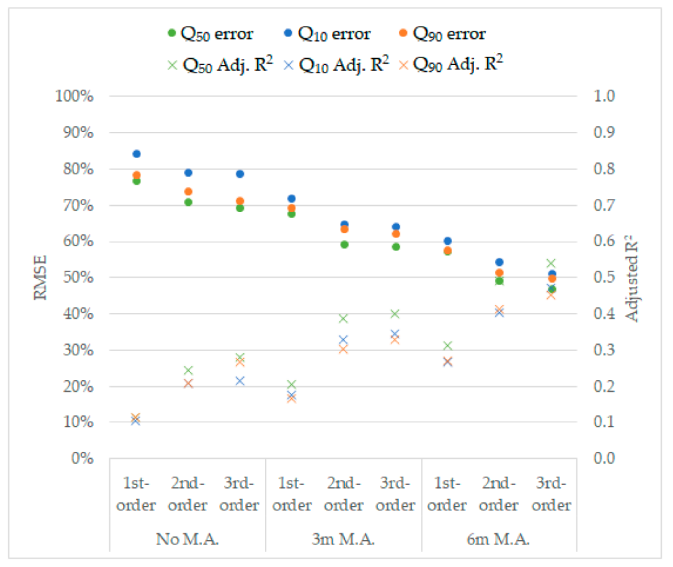
Figure 4.
Comparison between the observed variables and the estimated flow regimes by multiple polynomial regression model with 6-month moving average dataset. There are two figures: (a) The scatterplots of the estimated versus observed values; (b) The time series of observed (Q50, Q10, Q90, SOI, and DMI) and estimated (Q50, Q10, and Q90) values in 1994–2005 (left side of the separation line) and 2010–2018 (right-side of the separation line).


Figure 5.
Comparison between the observed variables and the estimated flow regimes by 6-month lagged multiple polynomial regression model with 6-month moving average dataset. There are two figures: (a) The scatterplots of the estimated versus observed values; (b) The time series of observed (Q50, Q10, Q90, SOI, and DMI) and estimated (Q50, Q10, Q90) values in 1994–2005 (left side of the separation line) and 2010–2018 (right-side of the separation line). The months showed at the x-axis are for the streamflow only. The months for the climate indices are 6 months before the streamflow months.
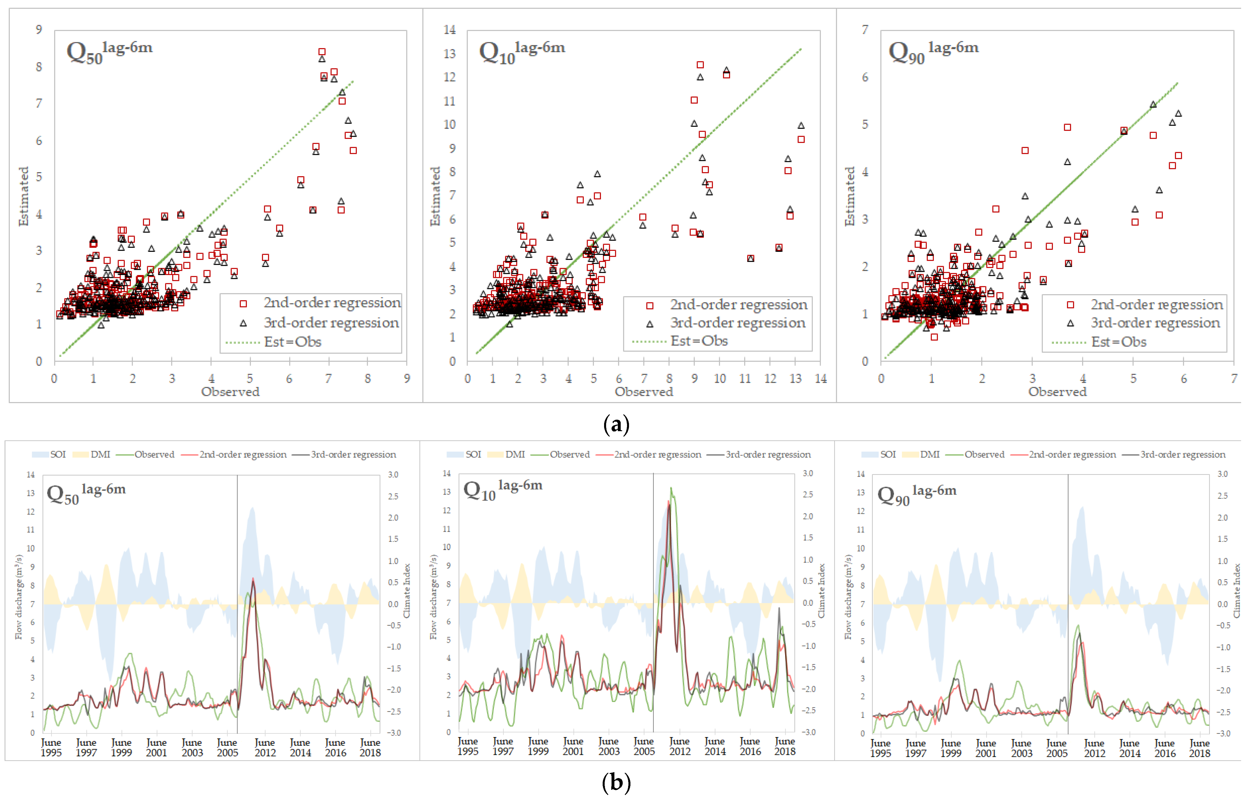
Figure 6.
Dummy simulations of second- and third-order multiple regression (6-month moving average) to show the modulation effect of DMI to SOI–streamflow relationship produced by the models. Dummy dataset of DMI (−0.8 to 0.8) and SOI (−2.0 to 2.0) were used in these simulations.
Figure 6.
Dummy simulations of second- and third-order multiple regression (6-month moving average) to show the modulation effect of DMI to SOI–streamflow relationship produced by the models. Dummy dataset of DMI (−0.8 to 0.8) and SOI (−2.0 to 2.0) were used in these simulations.


Table 1.
The coefficients of the correlation between the observed flow regime indices and climate indices (SOI and DMI) in the monthly datasets.
Table 1.
The coefficients of the correlation between the observed flow regime indices and climate indices (SOI and DMI) in the monthly datasets.
| Correlation Variables | No Moving Average | 3-Month Moving Average | 6-Month Moving Average |
|---|---|---|---|
| Q50 with SOI | 0.342 | 0.436 | 0.509 |
| Q10 with SOI | 0.330 | 0.407 | 0.466 |
| Q90 with SOI | 0.347 | 0.413 | 0.504 |
| Q50 with DMI | −0.031 | −0.047 | −0.029 |
| Q10 with DMI | −0.052 | −0.046 | −0.015 |
| Q90 with DMI | −0.099 | −0.109 | −0.104 |
The values in italic are statistically significant at the 95% confidence level with a two-tailed t-test.
Table 2.
The Pearson correlation coefficient (R) between the estimated and observed values of streamflow regimes on second- and third-order multiple polynomial regressions with SOI and DMI as predictors.
Table 2.
The Pearson correlation coefficient (R) between the estimated and observed values of streamflow regimes on second- and third-order multiple polynomial regressions with SOI and DMI as predictors.
| Flow Regime Indices | Multiple Regression Order | Correlation Coefficient (R) of Estimated-Observed | ||
|---|---|---|---|---|
| No Moving Average | 3-Month Moving Average | 6-Month Moving Average | ||
| Q50 | first-order | 0.350 | 0.459 | 0.564 |
| Q50 | second-order | 0.509 | 0.633 | 0.708 |
| Q50 | third-order | 0.553 | 0.650 | 0.746 |
| Q10 | first-order | 0.334 | 0.429 | 0.522 |
| Q10 | second-order | 0.474 | 0.586 | 0.644 |
| Q10 | third-order | 0.495 | 0.608 | 0.701 |
| Q90 | first-order | 0.347 | 0.418 | 0.527 |
| Q90 | second-order | 0.474 | 0.563 | 0.652 |
| Q90 | third-order | 0.542 | 0.594 | 0.688 |
All values are statistically significant at the 95% confidence level with a two-tailed t-test.
Table 3.
Multiple regression (MR) model evaluation for a 6-month moving average dataset in not-lagged (lag0) and 6-month lagged (lag6) MR. R is the Pearson correlation coefficient between the estimated and observed flow regime indices. RMSE is the root mean square error in percentage to the observed average. Adj. R2 is the Adjusted R2.
| Flow Regime Indices | Multiple Regression Order | Lag0 | Lag6 | ||||
|---|---|---|---|---|---|---|---|
| R | RMSE | Adj. R2 | R | RMSE | Adj. R2 | ||
| Q50 | second-order | 0.708 | 49% | 0.490 | 0.763 | 45% | 0.572 |
| third-order | 0.746 | 47% | 0.539 | 0.779 | 44% | 0.590 | |
| Q10 | second-order | 0.644 | 55% | 0.402 | 0.701 | 51% | 0.480 |
| third-order | 0.701 | 51% | 0.472 | 0.724 | 50% | 0.505 | |
| Q90 | second-order | 0.652 | 52% | 0.413 | 0.694 | 49% | 0.470 |
| third-order | 0.688 | 50% | 0.452 | 0.742 | 46% | 0.532 | |
Table 4.
Multiple regression (MR) model coefficients developed from a 6-month moving average dataset and lagged regression with climate indices lead streamflow indices by 6 months. To be used with the corresponding equations provided in the Section 3.2.
Table 4.
Multiple regression (MR) model coefficients developed from a 6-month moving average dataset and lagged regression with climate indices lead streamflow indices by 6 months. To be used with the corresponding equations provided in the Section 3.2.
| Flow Regime Indices | Multiple Regression Order | Coefficients | |||||||||
|---|---|---|---|---|---|---|---|---|---|---|---|
| β0 | β1 | β2 | β3 | β4 | β5 | β6 | β7 | β8 | β9 | ||
| Intercept | SOI | DMI | SOI2 | DMI2 | SOI.DMI | SOI3 | DMI3 | SOI2.DMI | SOI.DMI2 | ||
| Q50 | second-order | 1.449 | 0.225 | −0.457 | 1.133 | 1.588 | 2.189 | ||||
| third-order | 1.452 | −0.004 | −0.993 | 1.252 | −0.203 | 1.293 | −0.002 | 8.920 | −0.133 | 4.938 | |
| Q10 | second-order | 2.210 | 0.164 | −0.173 | 1.614 | 5.990 | 5.247 | ||||
| third-order | 2.182 | −0.001 | −1.406 | 1.777 | 0.699 | 1.978 | −0.135 | 19.498 | 1.865 | 15.137 | |
| Q90 | second-order | 1.141 | 0.316 | −0.263 | 0.616 | −1.181 | −0.080 | ||||
| third-order | 1.041 | 0.114 | −0.276 | 1.091 | −0.181 | 1.111 | −0.140 | 2.738 | −1.974 | −0.958 | |
Publisher’s Note: MDPI stays neutral with regard to jurisdictional claims in published maps and institutional affiliations. |
© 2021 by the authors. Licensee MDPI, Basel, Switzerland. This article is an open access article distributed under the terms and conditions of the Creative Commons Attribution (CC BY) license (https://creativecommons.org/licenses/by/4.0/).
Share and Cite
MDPI and ACS Style
Nugroho, A.R.; Tamagawa, I.; Harada, M. The Relationship between River Flow Regimes and Climate Indices of ENSO and IOD on Code River, Southern Indonesia. Water 2021, 13, 1375. https://doi.org/10.3390/w13101375
AMA Style
Nugroho AR, Tamagawa I, Harada M. The Relationship between River Flow Regimes and Climate Indices of ENSO and IOD on Code River, Southern Indonesia. Water. 2021; 13(10):1375. https://doi.org/10.3390/w13101375
Chicago/Turabian StyleNugroho, Adam Rus, Ichiro Tamagawa, and Morihiro Harada. 2021. "The Relationship between River Flow Regimes and Climate Indices of ENSO and IOD on Code River, Southern Indonesia" Water 13, no. 10: 1375. https://doi.org/10.3390/w13101375
Note that from the first issue of 2016, this journal uses article numbers instead of page numbers. See further details here.