Article

Groundwater Recharge in the Cerrado Biome, Brazil—A Multi-Method Study at Experimental Watershed Scale

1
Department of Forestry Engineering, Federal Institute of the North of Minas Gerais—Campus Salinas, Salinas 39560-000, Brazil
2
Department of Civil and Environmental Engineering, University of Brasília, Brasília 70910-900, Brazil
*
Author to whom correspondence should be addressed.
Water 2021, 13(1), 20; https://doi.org/10.3390/w13010020
Submission received: 27 October 2020 / Revised: 21 December 2020 / Accepted: 22 December 2020 / Published: 24 December 2020
(This article belongs to the Section Hydrology)

Abstract

:
Groundwater recharge is a key hydrological process for integrated water resource management, as it recharges aquifers and maintains the baseflow of perennial rivers. In Brazil, the Cerrado biome is an important continental recharge zone, but information on rates and spatial distribution is still lacking for this country. The objective of this work was to characterize the groundwater recharge process in phreatic aquifers of the Cerrado biome. For this, an experimental watershed representative of the referred biome was established and intensively monitored. The methodology consisted of an inverse numerical modeling approach of the saturated zone and three classic methods of recharge evaluation—hydrological modeling, baseflow separation, and water table elevation. The results indicated average potential recharge around 35% of the annual precipitation, average effective recharge around 21%, and higher rates occurring in flat areas of Ferralsols covered with natural vegetation of the Cerrado biome. As the level of uncertainty inferred from the methods was high, these results were considered a first attempt and will be better evaluated by comparison with other methods not applied in this work, such as the lysimeter and chemical tracer methods.

1. Introduction

Groundwater recharge is a key process that preserves stream baseflow and groundwater reservoirs. The correct characterization of this hydrological process is fundamental to integrated water resources management [1,2,3,4,5,6,7], although it is complex and difficult to quantify [8,9,10]. Temporal and spatial variability adds to the lack of data and resources, which prevents the actions taken by managers and researchers from being correctly fulfilled when facing scenarios of overexploitation, inordinate land use, pollution, and other environmental damage [11,12,13,14]. Depending on the particularities of a region, the extent of the groundwater recharge process can go beyond even national political and administrative borders [15,16]. The territorial extension of the Brazilian Cerrado biome illustrates this very well.
In the Cerrado biome, most of the soils are deep and permeable, which, along with other environmental factors, favors the infiltration and percolation of rain [17,18]. Considering the extent and geographic position of the Cerrado, it is an important groundwater recharge area that is responsible for the baseflow of some of Brazil’s main rivers [17,19,20]. Although the association of the Cerrado and water production is widely acknowledged, the historical environmental degradation that this biome has been submitted to is not reflected in the Cerrado’s strategic importance. The expansion of agriculture, livestock, industry, and urban areas has caused the loss of natural vegetation cover and increased the severity of soil erosion processes [21,22], both directly and associated with the reduction in long term water availability, mostly groundwater. To Cambraia-Neto and Rodrigues [20], the increase in water demand complements the series of issues that affect water resources in the region. Such scenarios represent a challenge to management institutions, influenced by the availability of data and knowledge [17,21,23,24]. In Brazil, efforts have been directed toward this issue in relation to the Cerrado biome.
Pinto et al. [25] assessed groundwater recharge in a basin representative of the Cerrado biome in Minas Gerais using monitoring data of the phreatic level in the area. Lousada and Campos [26] proposed conceptual models for water flow and movement in aquifers in the Cerrado biome in the Federal District by applying isotopic methods. Oliveira et al. [17] assessed the influence of land cover in the water balance of an undisturbed area in the Cerrado biome. In ANA [27], recharge was assessed using precipitation and infiltration rate data in a regional hydrological study performed to subsidize models for surface and groundwater integrated management in the São Francisco river basin, in the extensive Urucuia Aquifer System of the Cerrado. Carvalho and Scopel [22] studied recharge using water balance and assessed the influence of land cover in the recharge in a watershed in the Cerrado biome in the Goiás state. Using the same method, Ramires and Manzione [28] assessed recharge in a Cerrado area in the central-western São Paulo state. The results they obtained were corroborated by Gonçalves and Manzione [29], although the latter study adopted the method of water table elevation, which was also used by Matos et al. [8] in a hydrographic basin in the Cerrado biome. In another Cerrado region in the São Paulo state, Silva [30] studied the recharge process using a hybrid model for water balance and water table elevation. Cambraia-Neto and Rodrigues [20] used a water balance model to study recharge processes in a Cerrado basin in the west of the Federal District.
While the number of studies that have been carried out on groundwater recharge in the Cerrado is substantial, Oliveira et al. [17] highlighted that knowledge of the process and its interactions with the environment is still lacking considering the great diversity of characteristics the Cerrado biome over its continental scale. The fact that there is no universal method by which to study recharge [6,31,32,33] explains the adoption of various approaches, and encourages the simultaneous application of this methodological variety in an attempt to validate estimations of such a complex process, with high levels of uncertainty common [8,9,34]. Groundwater recharge estimation methods can be grouped into three categories: Physical, chemical, and numerical [31].
Physical methods include approaches based on measuring flows from which recharge is estimated indirectly [31,35]. Physical methods are represented by methods of water balance (vadose zone or saturated zone) [12,34,36,37], infiltration (vadose zone) [38,39,40], baseflow separation (saturated zone) [13,32,34,41], lysimeter measurement (vadose zone) [42,43,44,45], water table fluctuation (zone saturated) [8,34,46], and hydrological modeling (vadose zone) [14,47,48]. The positive aspects of this class of methods include its ease of application, the reduced number of parameters (baseflow and water table fluctuation [13,31,34,49]), and the possibility of characterizing the spatial variability (distributed water balance [14]). With some approaches, the estimate is accurate, but with local validity (lysimeter [31,44,49]), or it represents a general average for the basin (baseflow [49]). The reliability level depends on the accuracy of the flow measurement (water balance, baseflow, and lysimeter [31,49,50]) and the accuracy of the required data or parameters (hydrological modeling, baseflow, water table fluctuation [32,48]). For example, the water table fluctuation method can overestimate the recharge if the entry of water into the aquifer system does not cause a detectable rise in the water table (horizontal flow velocities higher than vertical flow velocities), or can underestimate recharge if water withdrawals in the recharge period mask the natural water table rise [10]. The lysimeter is the only direct method in this class, but it requires financial resources that are not always available for the structure installation [31,42].
Chemical methods are based on chemical tracers (natural or artificial) through which recharge is estimated indirectly by groundwater dating or empirical mass balance models [51]. In the latter case, with the estimated recharge based on relationships between the concentration of the tracer element in the atmosphere/precipitation and in the groundwater [2,23,52,53,54,55]. Among the most used tracers are deuterium (2H), tritium (3H), chlorofluorocarbons (CFCs), oxygen 18 (δ18), tritiogenic tritium/helium (3H/3He), and chlorides [31,51]. The methods in this group have low conceptual complexity, provide estimates with a high level of reliability, and good results for cracked and/or fractured aquifers. However, estimates are local or are averages for the studied environmental configuration and, for studies of natural tracers, they can only be applied in places where concentrations of the chemical elements in precipitation or in groundwater have detectable values [51].
When using numerical methods, the solution of the saturated or unsaturated flow equations is obtained from iterative computational numerical processes such as finite differences or finite elements [7,37,56,57,58,59]. The physical domain is simulated and discretized by means of regular or irregular cells, in which the flow is simulated and propagated three-dimensionally from Darcy equations or Richards’ equation variations using input data, calibrated parameters, and initial/known conditions for the simulation (boundary conditions) [31]. In this case, the model is implemented computationally through software, such as Modflow and Feflow, and recharge can be estimated by direct or inverse approaches. The main advantage of this methods class is the possibility of physical and spatial characterization of the recharge process. After being implemented, calibrated, and validated, the model can be used in the simulation of challenging scenarios for groundwater management such as land use/coverage changes and pumping [50,60]. On the other hand, they may require a high level of detail and monitoring in the study area and, consequently, an increased number of parameters and more input data, the quality and availability of which may compromise the reliability of results or even the method’s applicability [31,50,60].
One of the major difficulties with quantifying groundwater recharge is that each method is restricted to certain physical conditions of the study area, such as types of soil or climate, and can only evaluate a specific type of recharge, such as potential recharge or effective recharge, or can be used only for point estimates [5,9,31,34]. Some methods, for example, those based on flow direct measurements, can generate good results when obtaining point values, but may be unable to characterize the spatial variability of the process. Distributed methods are typically avoided due to the amount and variety of data required [7,12,13,29]. This methodological difficulty is not restricted to groundwater recharge research, and a way to overcome it is through the adoption of an experimental watershed as the study area. In this case, hydrological monitoring is more condensed because it is performed over a smaller area, and the environment can be selected to have physical and environmental characteristics representative of the basin or the biome to which they belong. Consequently, the data collected can serve as a basis for studies that may generate results that are valid for other non-instrumented areas with similar characteristics [61].
The present study aimed to characterize the groundwater recharge process in phreatic aquifers in the Cerrado biome using a multi-method approach and the proposition of an alternative approach, namely, adopting an experimental watershed representative of the biome.

2. Materials and Methods

The study area comprised the Capão Comprido watershed, a sub-basin of the Descoberto river located in the west of the Federal District between longitude 48°10′07” and 48°06′13” and latitude −15°43′42” and −15°45′41”, covering an area of approximately 16 km2 (Figure 1).
The climate in the region is classified as Aw humid to sub-humid, with well-defined rainy and dry seasons. The average temperature of the hottest and coldest months is 24°C and 10°C, respectively. Air relative humidity reaches critical levels of around 13%. Precipitation is concentrated between October and April, and the annual average between the years 1971 and 2016 was around 1500 mm [47]. The geological framework comprehends unities of sandy metarhytmites (metarhytmites are a regional type of geological formation, resulting from the metamorphization of stratified sedimentary rocks) and clayey metarhytmites, which belong to the Paranoá Group, and a small occurrence of Holocene alluvium close to the drainage network by the outlet of the Capão Comprido stream [62]. According to Reatto et al. [63], the predominant soil types are Red Ferralsol and Red-yellow Ferralsol, with a smaller amount of Cambisol, Plinthosol, and Gleysol. Regarding the natural vegetation land cover, the Capão Comprido watershed is predominantly rural, occupied by small farms, with remnants of riparian forests, typical formations of the Cerrado biome (open Cerrado grassland, shrub Cerrado, and Cerrado fields), pastures, reforestation areas, olericulture and perennial/fruit crops, and areas of bare ground [15].
The materials used consisted of field data and spatial information organized in thematic maps. Field data were collected as part of a continuous monitoring of the study area and comprised a historical series of precipitation, discharge, meteorology, piezometry, and hydrogeology. Geographical data comprised altimetry maps from SICAD—Federal District Cartographic System, geology [64], soil type [63], hydrogeology [64], and satellite imagery from the HRV/SPOT5 sensor. Model construction and simulations were performed using Visual MODFLOW v.4.2, WETSPA, and IDRISI, Andes version, and maps were prepared and elaborated using QGIS Desktop 2.18.23.
We used the following methods: (i) Saturated zone numerical modeling; (ii) hydrological modeling of the vadose zone; (iii) the water table elevation (WTE) method; and (iv) baseflow separation. The methodological steps are detailed in the subsequent sections.

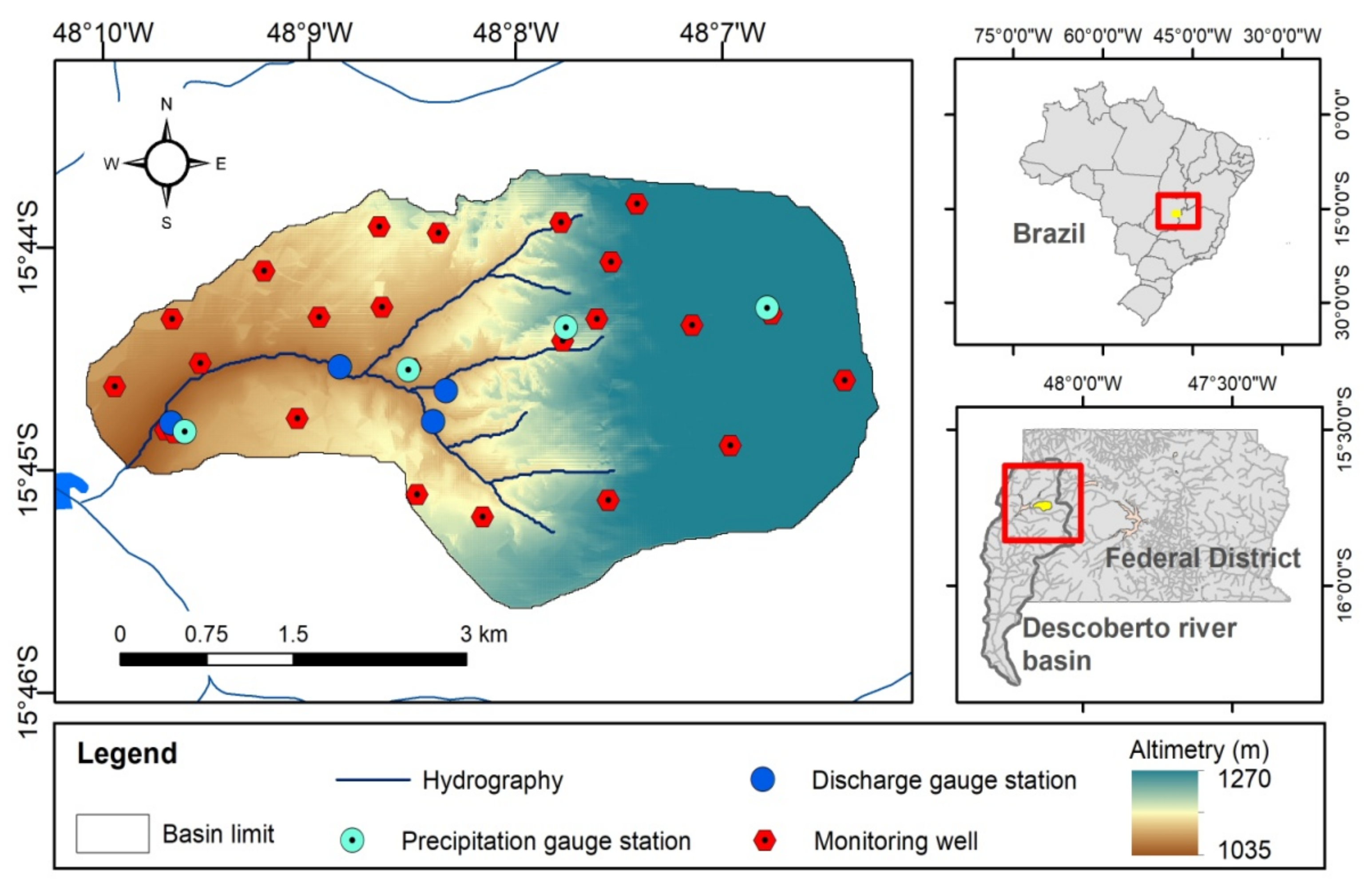
2.1. Monitoring and Data Collection

The network for data collection and monitoring consisted of four automatic tipping bucket rain gauges, five discharge stations equipped with water level logger, one complete automated meteorological station, and 23 monitoring wells, besides a few handmade water wells belonging to some residents. Precipitation data were registered at 15 min intervals and integrated into daily data. Discharge was measured in the river sections using an acoustic Doppler velocimeter with field visits matching the rainfall events or fortnightly in the drought period. We plotted a discharge rating curve using these data to convert water level daily values into daily discharge. The meteorological data were collected every 15 min and were used to calculate potential evapotranspiration by the Penman–Monteith method. Lastly, to survey piezometric data, the phreatic water level was measured fortnightly over the drought period, weekly in the rainy season, and at a sub-daily time scale in some wells using water level loggers. The monitoring period comprised the hydrological years of 2007/2008 and 2008/2009.

2.2. Numerical Modeling of the Saturated Zone

A numerical hydrogeological model of the phreatic aquifer in the study area was elaborated to simulate groundwater flows and recharge by vertical and horizontal numerical simulation using finite differences cells in Visual MODFLOW v.4.2 software. Modeling proceeded using the following reasoning: (a) Recharge is one of the processes responsible for alterations in the state of the aquifer system over time, and there are no available measured values of this process for the study area; (b) however, the “fixed” characteristics of the system (structural configuration and aquifer’s material properties) and temporal variation of its behavior (storage and phreatic level) are known, and other influencing factors are measurable (evapotranspiration and surface discharge); (c) thus, recharge is the unknown variable to be found. Al-aboodi et al. [65] used the same premise. Considering that recharge is usually input information, the problem can be solved with inverse modeling. Therefore, the spatial distribution was mapped, and recharge rates were estimated through calibration. The methodology developed is summarized in Figure 2.

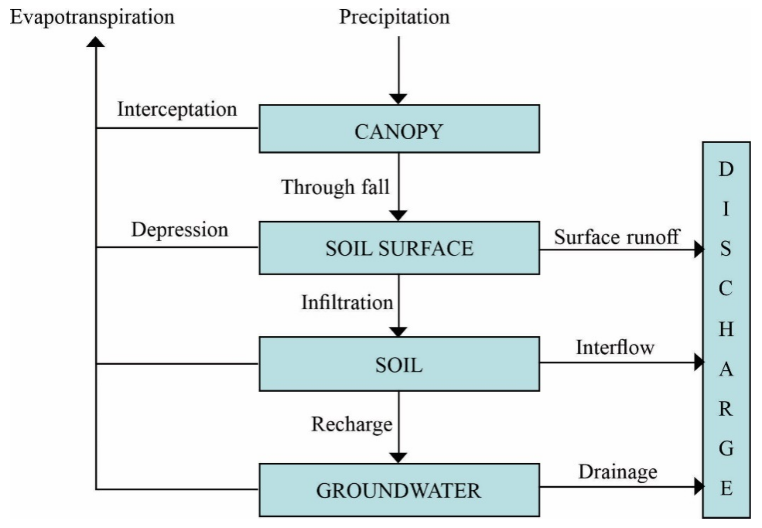
2.2.1. Conceptual Model

The conceptual model proposed (Figure 3) was based on various aspects of water flow. The water from precipitation, which percolates into the soil and reaches the saturated zone (recharge), flows through the subterranean porous medium until it reaches the surface drainage channel. Evapotranspiration occurs at a potential rate every time the plant root system intercepts the phreatic level. The horizontal border corresponds to the area limited by the lines from the surface water divider, while the vertical border comprises just the saturated zone, between the phreatic level and the impermeable lower base of the free aquifer. Time variations in the phreatic level, properties of the aquifer’s material, base discharge, and potential evapotranspiration are all known variables.
As it describes a complex system of interactions between surface and groundwater, data and parameters survey can reach a high level of detail. However, applying the principle of parsimony [67], we balanced between complexity and practicality. Excessively complex models require levels of data that are not always available [16]. In this regard, opting for the mentioned balance led to the adoption of the following assumptions: (i) The groundwater divider coincides with surface water divider; (ii) the aquifer is horizontally isotropic; (iii) aquifer discharges occur mainly into the local hydrographic network; (iv) groundwater abstractions and surface abstractions from perennial streams were irrelevant compared to the total water volume; (v) losses from the phreatic aquifer to the confined aquifer through deep percolation are irrelevant compared to the total water volume.
The vertical domain was divided into two layers, the first representing soil and the second representing the geological substrate. The thickness of each layer was estimated using a digital elevation model of the area [62,63,64] and geological information provided by companies that drill tubular wells in the Federal District. Horizontally, the aquifer parameters and properties map zones—saturated hydraulic conductivity (Ksat) and specific yield coefficient (Sy)—were spatialized using the soil type map [63] for the first layer and the geological substrates map [62,63,64] for the second. The values for the mentioned parameters were estimated in the field by performing pumping tests and slug tests using the monitoring wells. The time series data for potential evapotranspiration were obtained through the application of the Penman–Monteith method using meteorological data, and a potential evapotranspiration zones map was defined using the root system depth map, generated with the land use/cover map and based on Eiten [68], Canadell et al. [69], and Ferreira [70].
The recharge zone map was generated by performing a weighted linear combination of the maps for potentially determining factors of the process (slope, land use/cover, phreatic depth, hydraulic conductivity, and specific yield coefficient of the phreatic aquifer). The coefficients, or weights, were calculated by the AHP (analytic hierarchy process) multicriteria method. In this method, all factors are compared through a pairwise matrix according to a standard numerical scale of relative importance. Finally, from the values of the comparison matrix, the absolute weights of the factors are estimated by matrix operation [71,72]. Since the natural values of the factors in the maps are “not comparable”, we normalized the scales between 0 (unfavorable to recharge) and 1 (very favorable to recharge) using fuzzy functions—increasing sigmoidal function for factors with a direct relation, and decreasing sigmoidal function for factors with an inverse relation. This process was performed using geographic information systems tools available in the Idrisi software. A similar method was employed to outline recharge areas in Katmandu, Nepal, and in the Motloutse basin in Africa [3,24]. However, in these studies the maps were the result and were not used as input data for a better physical representation of the process in the numerical model, as proposed in the present work. The method to produce recharge zones maps is more detailed in Santos [15].

2.2.2. Numerical Model Implementation and Temporal Partition of Database

For this step, the conceptual model was computationally implemented using a regular grid with square cells, to which values were attributed for the aquifer parameters and boundary conditions. The solution for the flow in each node in the center of the cell was obtained by applying the “Finite Differences” method from the MODFLOW computational code using Visual Modflow software [73].To achieve this, we carried out the following steps:(i) Horizontal and vertical domains definition; (ii) the definition of the model’s cell grid spatial resolution and the number of layers and position of the vertical domain; (iii) the definition of the zones (spatial distribution) and values for the Ksat and Sy parameters in the model’s free aquifer; (iv) insertion of the boundary conditions zones maps (surface drainage/discharge areas, evapotranspiration, recharge, and initial piezometric head); and (v) the input of time series data (evapotranspiration, drainage hydraulic head, piezometric head in the monitoring wells, and recharge rate).
The 20 m grid cell size was defined by simulation tests, beginning at a low-resolution grid and refining the line and column spacing until no relevant alterations were observed in the results. The values for parameters and boundary conditions in the cells were attributed from the respective zones’ maps, as outlined in the conceptual model. In the case of drainage, the channel was identified in the numerical model by selecting the cells located over the lines that represent the perennial hydrographic network, and the implementation of this boundary condition was done using the “River” module in Visual Modflow [15]. The hydraulic head in the drainage channels was defined by water level time series, obtained from discharge gauge stations distributed along the drainage in the study area.
We used one day as the time interval, and this time step definition was based on recommendations from Hill and Tiedman [74]. This time resolution adjusts to the input data characteristics. When smaller intervals were tested, no considerable changes were observed in the model’s response.
Last, three simulation steps were established, which served as a guide to database partition in three parts: (i) Part I—drought period of 2008 (July to October) to adjust the model and the aquifer property values; (ii) Part II—drought period of 2009 (July to September) to verify the calibration performed in Part I; (iii) Part III—rainy period of 2008–2009 (from October 2008 to May 2009) to estimate recharge using inverse modeling by automated calibration. Aiming to eliminate or reduce the effects of the initial condition in the model’s response, “warm up periods” were implemented in each of the numerical modeling steps (Calibration 1, Verification and Calibration 2), successively replicating the data. The analysis of the results considered only the last cycle.

2.2.3. Numerical Modeling

A sensitivity analysis was carried out before the first calibration to assess the impact of the Ksat and Sy parameters on the modeling. This procedure was performed by manually varying the initial values (estimated in the field) of the referred parameters by ±10%, then observing the model’s response. After the sensitivity analysis, the values for the aquifer’s parameters—Ksat and Sy—were adjusted by calibration and verified with data from drought periods, which usually have no recharge. The aim was to eliminate recharge as an unknown variable, since it was considered zero during the mentioned period. Therefore, the remaining adjustable parameters were Ksat and Sy. The main consequence of this solution was the reduction of individual uncertainty in the calibrated parameters, which was generated when more than one parameter was calibrated together. Adjusting several parameters simultaneously may lead to estimations that do not assume unique values for each parameter, considering that individual values can be adjusted and combined in many ways to make up the optimal solution for the model [58,74,75]. Using the calibrated model, recharge rates were estimated for the previous zones map by calibration. This second calibration was called “inverse modeling”, and was based on the execution of the parameter estimator in Visual Modflow, WinPEST parameter estimator [76].
In all modeling steps, the initial head was defined by kriging interpolation of the piezometric head measured in the monitoring wells. The phreatic level time series and discharge time series were adopted as reference values to assess the quality of the model’s adjustments.

2.3. Distributed Hydrological Modelling of the Vadose Zone

This step was based on the application of a physics-based distributed model with empirical implementation and routines to simulate water flows between the atmosphere, vegetation canopy, root zone, transmission zone, and the saturation zone (Figure 4). The model was called WETSPA (water and energy transfer between soil, plants, and atmosphere) [77].
The input data were composed spatial data and hydrological time series data. The spatial data reflected physical characteristics of the basin such as slope, soil type, land use, and cover, in the form of digital maps in raster structure. The hydrological data consisted of tabulated time series precipitation and potential evapotranspiration data. The simulation processed data at the cell level, with the spatialization of precipitation and potential evapotranspiration time series and the basin’s physical characteristics maps, which were used to spatialize mathematical parameters related to the model formulation and water movement through the physical reservoirs. The model computes water balance in each cell using the following equation:
DΔθ/Δt = P − I − V − E − R − F
where D [L] is the root system depth; Δθ [L3L-3] is the variation in soil moisture content; Δt [T] is the time interval adopted in the simulation; P [LT-1] is precipitation in the time interval adopted in the model; I [LT-1] are initial abstractions including interception and storage in soil depressions; V [LT-1] is surface runoff or effective precipitation; E [LT-1] is the actual evapotranspiration; R [LT-1] is the percolation below the root zone; and F [LT-1] is the sub-surface flow.
Interception is calculated as a function of the leaf area index, precipitation, and potential evapotranspiration, considering that leaf area index is a defined parameter that can be calibrated based on land use and cover (vegetation). For the storage in soil depressions, mass balance is calculated as a function of the depression’s storage capacity in each cell (can be calibrated in function of land use and cover), effective precipitation, evaporation of the water stored in the surface depressions, and infiltration of the water stored in the depressions during the time interval adopted for the simulation.
Effective precipitation was calculated using a variation of the rational model, in which the surface runoff coefficient is adjusted as a function of the slope, soil type, land use/cover, precipitation order of magnitude, and previous soil moisture content.
Actual evapotranspiration was computed as a function of the potential evapotranspiration, a coefficient of the vegetation type defined using the land use/cover map, the current soil moisture content in the cell, the soil moisture content at field capacity, and the soil moisture content at permanent wilting point; the latter two parameters can be calibrated and are defined as a function of the soil type.
Regarding percolation, the model considers that it is processed between the root zone and the saturated zone according to Darcy’s law. It is the product of hydraulic conductivity and hydraulic potential gradient. However, if the gradient varies little in the soil, its value is close to one, considering that percolation is controlled only by gravity. This way, percolation starting in the root zone was estimated using hydraulic conductivity related to the average soil effective saturation using the Brooks and Corey equation. Concerning the sub-surface flow, WETSPA assumes it occurs after the beginning of percolation and ends when the soil moisture content is lower than the field capacity. The following equation was used to estimate sub-surface flow and is based in Darcy’s law and the approximation of the cinematic wave:
RIi t = kiDiSiK θ i t Δ t / Wi
where Si is the cell slope (L/L); K[θi(t)] is the cell effective hydraulic conductivity to a moisture content of “θi(t)” (L/T); Wi is the cell width (L); and ki is the coefficient that is related to land use and cover, drainage density, and the effect of organic matter and the root system on the hydraulic conductivity in the soil surface layer.
The flow propagation through the cells and the drainage channel was performed by an approximation of the St Venant equation “diffuse wave”:
Q t = d 2 Q X 2 c Q X
where Q [L3T-1] is the discharge at time “t” and location “x”; t [T] represents the time interval adopted in the simulation; x [L] is the distance in the direction of the flow; c [LT-1] is the wave velocity or “disturbance” along the flow path; d is the dispersion coefficient depending on location that expresses the tendency to disturbance, or wave longitudinally dispersed downstream. Considering that the hydraulic radius is equal to the height of the flow in the cell or in the channel, c and d were calculated by c = (5/3)v and d = (vH)/(2S0), where v [LT-1] is the flow velocity calculated by the Manning equation, and H [L] is the hydraulic radius.
Surface runoff at the beginning of the flow was obtained by a linear approximation of the diffuse wave equation:
U ( t ) = 1 σ 2 π 3 / t 0 3 exp ( t t 0 ) 2 2 σ 2 t / t 0
where U(t) [T-1] is the instantaneous unitary hydrogram for the flow propagation in any cell downstream or at the basin’s outlet, and t0 [T] and σ [T] are the average and standard deviation of the flow time; the latter two parameters are spatially distributed and were obtained as a function of the flow velocity and the dispersion coefficient.
The groundwater flow in the saturated regime (aquifer recharge and discharge for the surface drainage network) was computed in a simplified way, as a linear reservoir in each sub-basin, propagated downstream.
The parameters required by WETSPA are divided into two groups, local and global. The local parameters are those for which the spatial distribution is processed at the cell level, provided by tabulated data and spatialized as a function of the soil type, slope, and land use/cover. The global parameters consisted of parameters that would be difficult to spatialize the values for each cell. Thus, the estimations are valid for the entire basin. Table 1 summarizes the groups and how they were estimated.
The model description was executed based on Liu and Smedt [77] and Bahremand et al. [78]. More details of the mathematical formulation and assumptions are available in the referenced studies.
The model was fed with geographic data of the area—maps of soil type, slope, and land use/cover—and with the time series precipitation and potential evapotranspiration data. Calibration was executed starting with a sensitivity analysis aiming to identify determining global parameters, using the series from the hydrological year of 2007/2008. We used the model default values to estimate the local parameters [77]. The verification was simulated using the calibrated model for the hydrological year of 2008/2009. The time series of measured and estimated flow rates using the discharge rating curve was used to assess the performance of the model in both steps. The result was also evaluated by comparison with the recharge simulated for a neighboring basin, localized in the same biome and with similar climatic and physical characteristics [47].

2.4. Water Table Elevation (WTE)

We estimated the piezometric elevation over the recharge period during the rainy season using the phreatic level monitoring data. The observed elevations in each monitoring well were obtained graphically, corresponding to the vertical distance between the maximum piezometric head and the prolonging of the piezometric curve recession line, as indicated by Matos et al. [8] and Healy and Cook [79]. Point recharge, valid for the influence area of the monitoring well where the water table elevation was observed, was estimated by multiplying the total elevation(mm/year) by the local value for the aquifer specific yield coefficient, Sy. Values of Sy were obtained by pumping tests and slug tests, executed by Santos [15] in the monitoring wells at the Capão Comprido watershed.
Since the number of recharge point estimates was relatively small to guarantee a good performance of regular interpolators, another way of spatializing the recharge point values has been proposed using a spatial multiple regression model, of the type “Y=a+b1X1+b2X2+b3X3+...bnXn”, with recharge as the dependent variable of the spatial distribution of the factors previously defined as being determinant to the mentioned process (slope, land use and cover, aquifer hydrodynamic behavior, aquifer thickness, and phreatic depth). A similar approach was adopted by Lacombe et al. [32]. Since the natural order of magnitude, scales, and units associated with the mentioned factors differ, these data were normalized according to the inverse or direct influence of the factor on the recharge by fuzzy functions (normalized scale varying from “zero” to “one”). More details about the proposed method are presented in Santos [15].

2.5. Baseflow Separation

The hypothesis adopted was the existence of a connection between groundwater and surface water in the study area. The estimations for baseflow were performed both using field observation and in an indirect estimation of the total recharge occurring over the entire basin [80].
The estimations of baseflow were obtained using a mathematical filter [81] for the baseflow separation applied to the total discharge time series at the basin outlet:
q t = β · q t 1 + 1 + β 2 · Q t Q t 1
where q represents the direct surface runoff, β represents the adjustable parameter, and Q represents total discharge.
The baseflow was obtained by subtracting the calculated direct surface runoff from the total discharge. Values for “β” could vary between zero and one, considering that it is inversely proportional to the aquifer’s contribution to the total discharge, that is, the bigger “β” is, the lower the fraction of baseflow contribution to discharge in river floods. The value adopted for “β” was 0.98 based on Santos [66], since the participation of baseflow in flood events is low in relation to the total discharge in the study area.

3. Results and Discussion

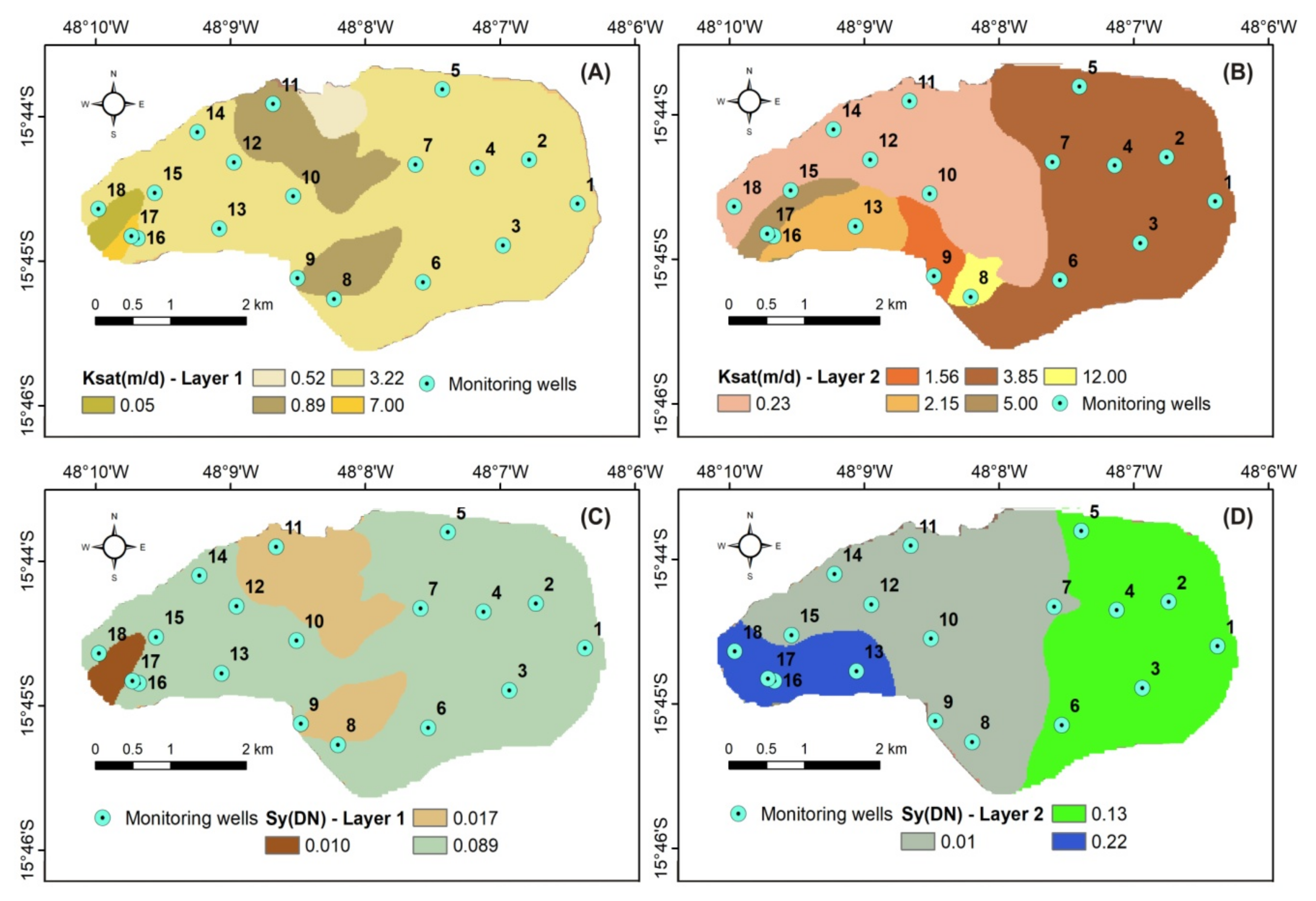
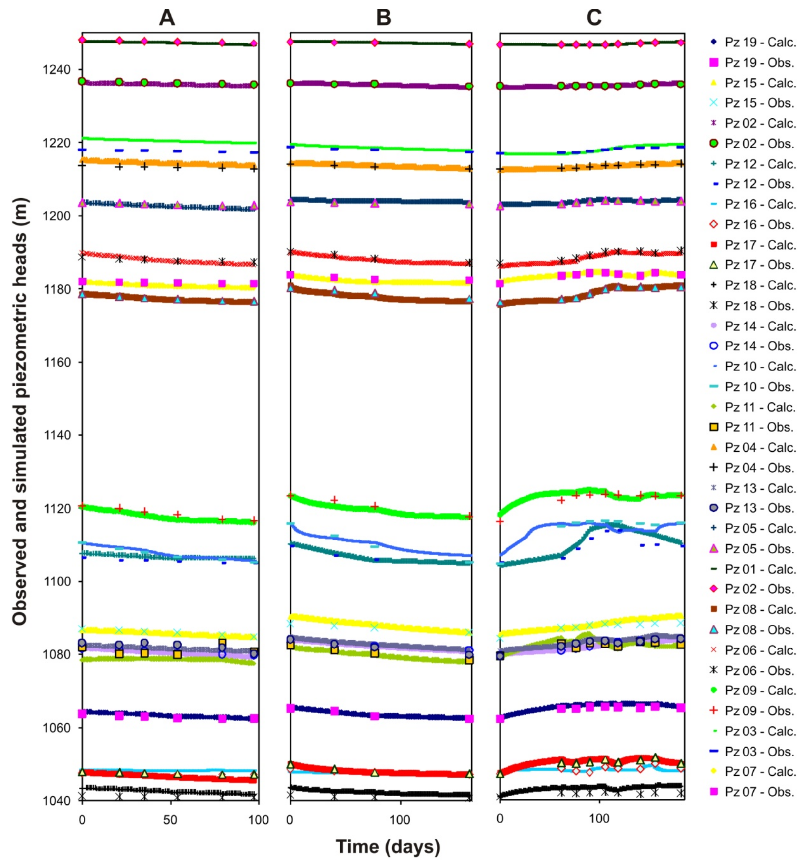
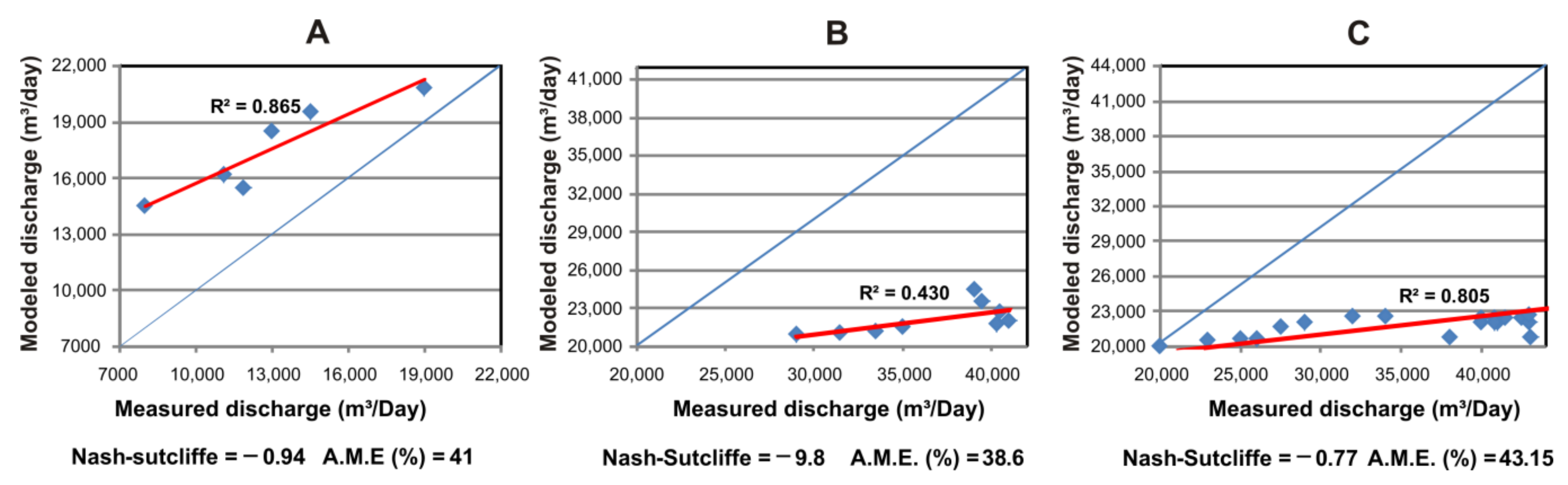
3.1. Numerical Modeling

After implementing the numerical conceptual model, three simulations were executed. For the first simulation, we aimed to adjust the values and the spatial distribution of the aquifer properties (Ksat, Sy, and vertical stratification) with manual calibration. For the second, we aimed to verify and validate the calibration using another historical dataset, and for the third, we executed the calibrated model to estimate the recharge rates of the previously determined zone by automated calibration (inverse modeling).
In the first calibration, only the parameters of the second layer were adjusted, because few piezometers were used in the pumping and slug tests have a depth compatible with the first layer’s depth (where the flow in unsaturated regime is predominant), and because in the sensitivity analysis, the Ksat and Sy values for that layer did not have a significant impact on the model’s response. Thus, for the first layer, mean values were adopted for the zones, based on the point estimates in the shallow piezometers and the soil map (Figure 5A,C). For the second layer, mean values calculated from the field values estimated by slug and pumping tests were assigned to the zones based on the geological map. The average zones values were adjusted, and the ones that better simulated piezometric heads and drainage discharge are presented in Figure 5B,D. The differences between average field values and calibrated values are presented in Table 2.
The differences between calibrated and average assigned values of Ksat and Sy varied from 8% to 112%. Considering that these aquifer properties are parameters that can present high spatial variability, the field estimations served as an indicator of the order of magnitude required for the calibration process. Although other attempts at adjustment were made, this was the best result we obtained. The calibrated parameters that simulated piezometric head and drainage discharge in the calibration are presented in Figure 6, while the verification and inverse modeling steps are presented in Figure 7.
For the piezometric head in the calibration step (Figure 6A), the module residuals were generally low. The greatest frequency (74% of total comparisons between observed and simulated) was of lower residuals, around 10%, related to the maximum variation of the phreatic level in the study area (11.8 m), while only 9% presented residuals more than 20% over the reference value. The maximum residual (−37.6%) was observed in a piezometer under the influence of a small lake. Regarding the drainage discharge (Figure 7A), the absolute mean error was 41%, and Nash–Sutcliffe efficiency index was −0.94.
In the verification step (Figure 6B), the model presented the same performance as the previous step. It was able to simulate the piezometric heads well, but underestimated drainage discharge. For 89% of the comparisons between simulated and observed heads, the residuals were lower than 10%, the maximum absolute residual was 18%, the minimum was 1% and the average was 4%. For the piezometric heads in 13 piezometers, the Nash–Sutcliffe efficiency index was between 0.6 and 0.99; in two of them, the relative mean error was higher than 10%. Regarding the base discharge, the percentage absolute mean error was 39% and the Nash-Sutcliffe index was −9.8. The low performance of the model with regard to simulating the base discharge was assigned to the processes of storage and flow retardation, and the uncertainty of the thickness and depth of the model’s layers. Although the need for adjustments in general is evident, it was not possible to obtain better results, which is the reason why the calibrated model was used to estimate recharge rates in the previously mapped zones.
The calibrated and verified model was used to estimate recharge for the hydrological year 2008/2009 using the hydrological data. In the piezometric head simulation, 84% of residuals were below 10%, with an absolute mean residual of 2%. Only one piezometer presented an unsatisfactory Nash-Sutcliffe efficiency index. For the drainage discharge, the absolute mean error was around 43%, and the Nash–Sutcliffe index was −0.77. The probable cause of the low performance of the model to simulate baseflow was that the parameters Ksat and Sy, as well as the thickness and depth of the model’s layers, still needed adjustment.
The greatest values of groundwater recharge were observed in the area near the water divider and the contact lines between geological formations with different hydrodynamic behavior such as sandy metarhytmite and clayey metarhytmite. The spatial distribution of the total annual recharge, represented in percentage of the total precipitation occurred in the hydrological year of 2008/2009, is displayed in Figure 8.
The recharge rate varied between 0 and 79%, with total recharge in the basin of around 21% of total annual precipitation. Considering that the model underestimated drainage discharge and despite the good performance in the simulation of piezometric heads, it was considered that the total recharge in the watershed is higher than the estimated value. In this case, there are no reference values with which to assess the reliability of the results for the study area. However, since it is an estimation of effective recharge, values obtained with the WTE method can at least highlight the likely approximation of the recharge rate. In the present work, the recharge estimated by this method was 15%. When applying the method to a watershed with similar soil classes distribution that is also in the Cerrado biome in the east of the Federal District, Cambraia-Neto and Rodrigues [20] estimated an average recharge of 26.6%. In ANA [27], the effective recharge for the Cerrado area over the Urucuia Aquifer System was estimated to be16%, although the method used was not WTE. Even in Araujo [47], who used SWAT-MODFLOW to estimate effective recharge in a basin the borders the Capão Comprido basin, recharge was 19%. Al-aboodi [65] described that the greatest limitation of inverse numerical modeling for recharge simulation is to depend on the parameters Ksat and Sy and other boundary conditions. Since the characterization of the aquifer environment in the study area had gaps, the resulting recharge estimations had high levels of uncertainty. In the sensitivity analysis, it was found that a 10% variation in Ksat causes an 18% change in recharge. For Sy, the same variation has an impact of 12% on recharge.
In general, parameters related to the aquifer environment, such as soil type and geological substrate, were determining factors in regulating recharge, responsible for the greatest mean values. On the other hand, the lowest values were regulated by slope and type of substrate. There was no clear relationship between land use/cover and recharge rates, since relatively high values were observed both for riparian forest and pastures. Regarding saturated numerical modeling, this is not incoherent, since recharge in one cell can be a result of side flows from neighboring cells with different land cover types.

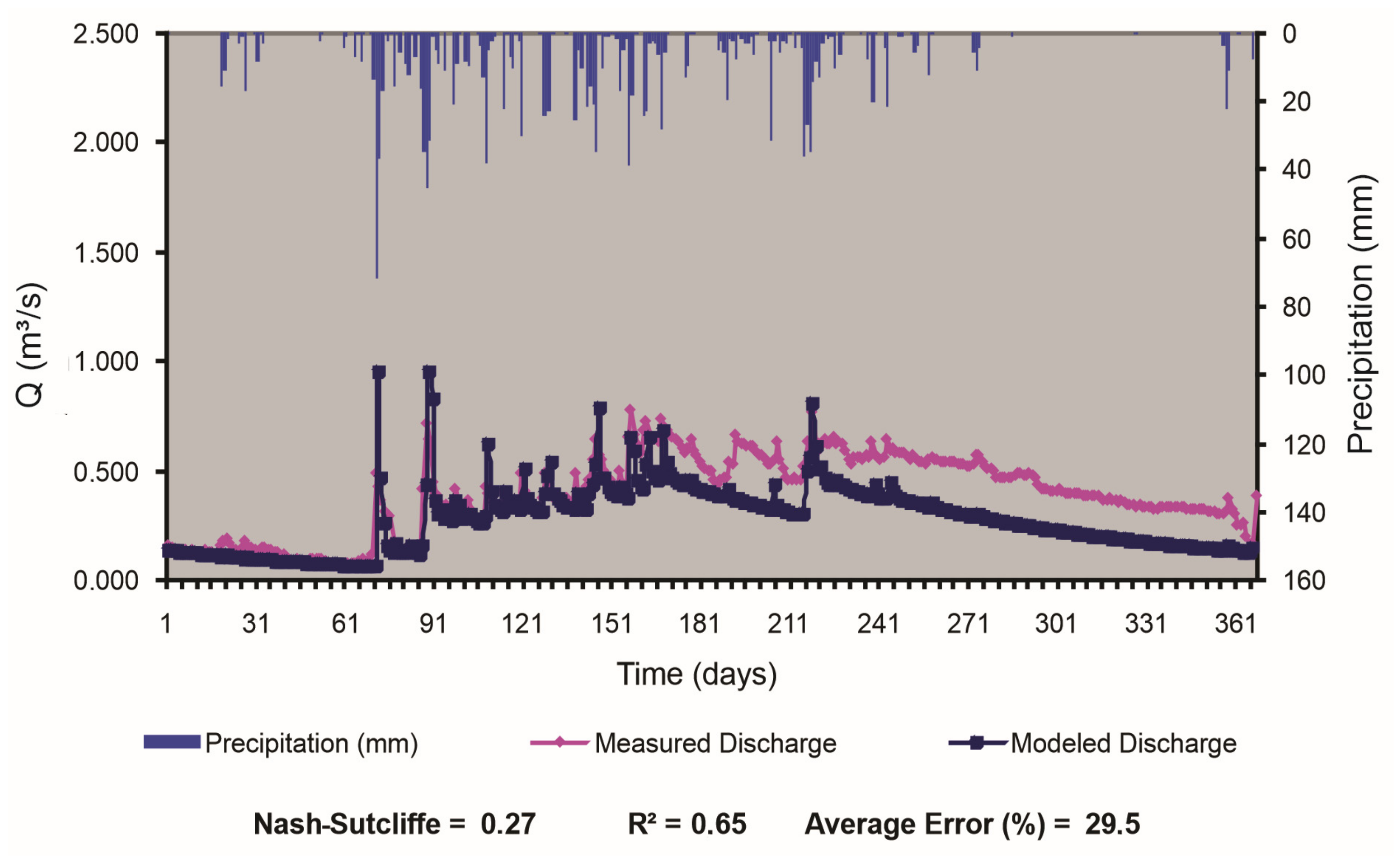
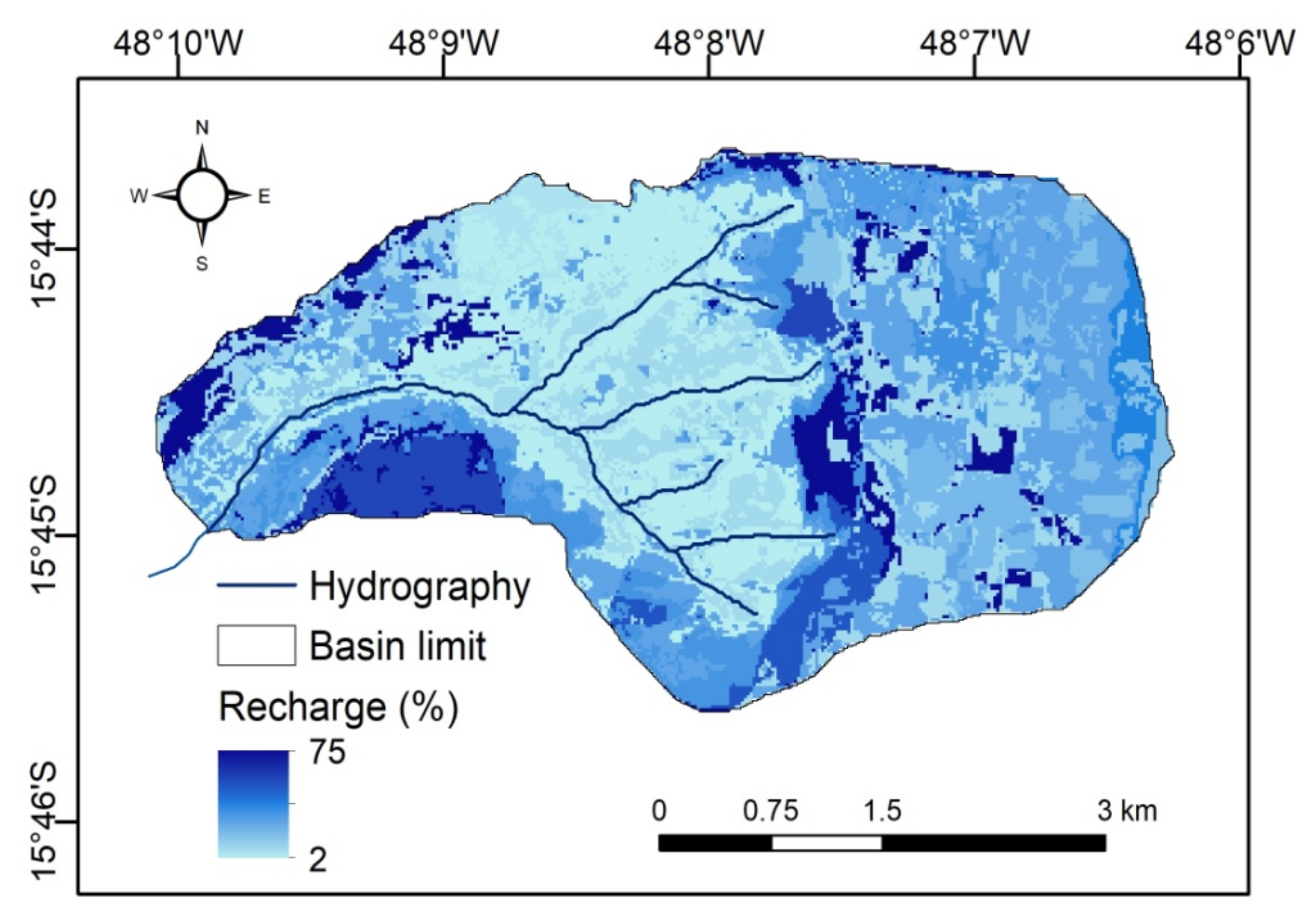
3.2. Hydrological Modeling

The sensitivity analysis (Table 3) highlighted that the parameters “Porosity”, “Pore size distribution index”, “Root system depth”, “Coefficient to correct potential evapotranspiration (Kep)”, “Aquifer recession coefficient (Kg)”, and “Aquifer initial storage (G0)” have the greatest impact on the model’s response. However, following the recommendations of Liu and Smedt [77], it was decided to calibrate only the global parameters. The calibrated values that supported the satisfactory performance of the model are shown in Table 4.
For parameters with defined reference values, the adjusted values were located within the expected ranges. The others were adjusted based on the hydrological behavior of the watershed, observed in the field, and based on values adjusted for other regions, according to Safari et al. [82]. After adjusting the parameters related to evapotranspiration and porous medium characteristics, we ran a simulation for the hydrological year of 2007/2008 (Figure 9).
For the calibration, the Nash–Sutcliffe efficiency index and percentage absolute mean error were deemed satisfactory, with values of 0.70 and 14%, respectively. Local parameters were not adjusted, since they were not measured in the field and reference values were unavailable for the study area. The values for adjusted global parameters were applied to the verification step, this time using data for the hydrological year of 2008/2009 (Figure 10).
The model presented satisfactory performance until day 151, from which the difference between the measured and modeled discharge increased, modeled discharge being lower than the measured discharge. A new calibration was executed to improve the adjustment in the verification step. However, even after testing a large range of values in the parameters, a better result was not achieved. The total annual volumes for both periods were practically the same (1551 mm and 1581 mm, respectively). Nonetheless, during the verification period rainfall was less intense and distributed more evenly over time, generating fewer discharge peaks and more infiltration. The spatial distribution of the recharge during the verification period is displayed in Figure 11.
The recharge rate varied between 0 and 45% of the total annual precipitation, with an average of 35% for the entire watershed. In the same biome, same region, and using methods similar or equivalent to hydrological modeling, Araujo [47] obtained an average recharge rate of around 38% in a watershed bordering the Capão Comprido. For a basin in the east of the Federal District, Cambraia-Neto and Rodrigues [20] estimated a recharge rate of 30%. In other regions, but still in the Cerrado biome, Carvalho and Scopel [22] reached a similar result of 36% in a basin in the Goiás state with similar soil classes as those studied here. In São Paulo, Ramires and Manzione [28] estimated a recharge rate of 36% using a water balance model with precipitation data from remote sensing (TRMM). For a Cerrado area in the state of São Paulo, Silva [30] simulated rates of 35% and 49% for areas with forestry and preserved Cerrado, respectively. In the state of Minas Gerais, Souza et al. [83] simulated a potential recharge rate of 30% for Ferrasols in the Rio Doce basin. Although this last case was in the Mata Atlântica biome, it indicates that Ferrasols may exhibit the same hydrological behavior regardless of the biome where it is encountered.
Even if references indicate that recharge mean values simulated with hydrological modeling can be reasonable, the most probable distributed recharge rates are uncertain and could be situated in a range from 0 to 49%, considering only the results obtained in the present work and in the referenced literature. However, since the model underestimated base discharges for the analyzed data period, it is likely that the simulated recharge rates, both in terms of the basin’s mean values and the distributed local values, have a high level of uncertainty and were underestimated.
The spatial pattern was strongly influenced by the soil type, with the greatest values occurring in Red Ferralsol, Yellow Ferralsol, and Plinthosol soils with medium texture, while the lowest values were in Cambisol. An average recharge rate higher than that simulated with numerical modeling was expected since hydrological modeling simulates potential rates only.

3.3. WTE Method

The WTE method was used to account for the fact that recharge at any given point is equal to the product of the local water table elevation fluctuation (Δh) and the aquifer’s specific yield coefficient (Sy). Table 5 presents the recharge results for the hydrological year of 2008/2009 after using the WTE method.
A spatial linear regression model was generated to spatialize point estimations, conditioning the recharge rate to factors related directly to it. According to the obtained model, recharge in the study area can be expressed with
Rc (mm) = 173.98−10.23 × D + 0.039 × Esp + 5.66 × Ksat + 6.18 NF
−5.99 × Sy + 5.34 × UT + 0.0029 × S
where Rc represents recharge (mm/year); D represents slope; Esp is the aquifer thickness; Ksat represents the saturated hydraulic conductivity; NF is the phreatic depth; Sy is the specific yield; UT is the land use and cover (classes ranked in terms of favoring recharge); and S represents the soil type (classes ranked in terms of favoring recharge).
The dependent variable was analyzed using t statistics, calculated for each regression coefficient, considering ∞ degrees of freedom and a 99% level of trust. The calculated t absolute values that surpassed the default critical value (2.33) were relative to D (t = 233) and NF (t = 140), followed by “Ksat” (t = 46), “UT” (t = 43), “Sy” (t = 32), “Esp” (t = 19), and “S” (t = 4). This order indicates each variable’s relative importance to the spatial distribution of the dependent variable, and suggests that the last two (“Esp” and “S”) are the only ones that could be excluded from the model without altering the correlation coefficient (R) and predicted values. The determination coefficient obtained was 0.99, and the map generated with the model is presented in Figure 12, displaying express recharge as a percentage of total annual precipitation.
The recharge rate varied between 0 and 29%with a mean value of around 15%. This mean estimation is similar to the effective recharge estimate of 16% made by ANA [84] for Cerrado areas in the Urucuia Aquifer System, and is lower than the estimate from Cambraia-Neto and Rodrigues [20] of around 26.6% of the total annual precipitation for a basin with Red Ferralsol also in the Cerrado biome, in the eastern Federal District. In this last case, the difference may be lower in comparison with the present work’s estimations, since in the Capão Comprido watershed the areas with Red Ferralsol, a predominant characteristic in Cambraia-Neto and Rodrigues [20], had recharge rates between 15% and 29%. Besides, the number of monitoring wells and, consequently, the quantity of water level data and field estimations of Sy needed to execute the model were higher in the Capão Comprido watershed. In Araujo [47], the effective recharge simulated with SWAT-MODFLOW was around 19% for the Ribeirão Rodeador basin, which borders the Capão Comprido basin.
Recharge rates estimated by the WTE method are effective but, according to Healy and Cook [79], the method tends to underestimate recharge rates for sites with high saturated hydraulic conductivity, since water input events could occur without phreatic level raising, that is, the vertical input rate equals horizontal output rate. In addition, human interference in the aquifer system can, if not considered, cause errors in the water table time series and the estimated recharge [10]. Such errors can be minimized with the incorporation of variables such as precipitation, evapotranspiration, abstraction, and anthropogenic interventions in the environment. Yihdego et al. [60] and Yihdego and Khalil [10] suggested tools to deal with this. In general, there was a predominance of Red and Red-yellow Ferralsol associated with the highest values.

3.4. Baseflow Separation

The baseflow separation filter for total discharge data from the hydrological years of 2007/2008 and 2008/2009 are displayed in Figure 13 and Figure 14, respectively.
The total precipitation volumes in the first and second periods were 1551 mm and 1589 mm, respectively. Despite the precipitation values being close, the average baseflow in the second year was 21% higher than the first year (0.30 m3/s in 2008/2009 vs. 0.24 m3/s in 2007/2008, respectively). This difference can be explained by the fact that rainfall in 2008/2009 was less intense and more evenly distributed over time, favoring infiltration and percolation processes. Furthermore, rainfall was concentrated in the beginning of the rainy season, when the soil is still dry and more susceptible to infiltration, causing a greater water input and, consequently, greater recharge. This result diverges from that obtained by Gonçalves and Manzione [29], according to whom the percentage of recharge does not vary considerably as a function of variation in annual precipitation. Total annual recharge estimates were calculated for the estimated baseflow values and are presented in Table 6. The difference in recharge estimates for both years was approximately 19%.
The filter used for baseflow separation might have overestimated recharge rates. Since it calculates effective recharge, it was expected that its value would be lower than the estimations made by potential recharge methods such as hydrological modeling. In this regard, the most probable annual recharge rate calculated by baseflow separation was close to the estimate made by Santos [85] for the same study area of around 25% of annual precipitation. This value is close to the one estimated by Cambraia-Neto and Rodrigues [20] using a similar mathematical filter for a basin in the eastern Federal District. Nonetheless, divergences in estimations obtained using different filters are common [32]. Spatial distribution could not be estimated due to a lack of discharge data, since discharge is measured in the outlet of the entire basin, where the flow measurement station is installed.

3.5. Comparative Analysis

When different methods are applied to estimate groundwater recharge in the same study area, it increases the validity of results, because besides each method’s individual contribution to comprehend the process, they can also be complementary or serve as a verification standard for others. In this regard, considering the results found in the present work, we sought a response to three fundamental issues: (i) What is the average recharge rate for the study basin and, consequently, for similar areas in the Cerrado environment? (ii) Which spatial distribution of the process is most reasonable to use? Finally, (iii) which method is best for the conditions found in the study area and similar Cerrado biome areas?
The selected methods enabled the estimation of two types of recharge: Potential recharge, simulated by distributed hydrological modeling; and effective recharge, simulated by numerical modeling, WTE method, and baseflow separation. The results using these methods are summarized in Table 7.
With regard to potential recharge, although the average value was underestimated, the 35% recharge rate was deemed plausible considering the similarity to values obtained by various authors, including for areas in the same region. The value maybe updated through improvements in the model’s calibration process, or by comparing with more precise direct local methods, applied locally for all the diversity of environmental conditions in the area, such as the lysimeter [68]. With regard the effective recharge, despite the significant methodological differences between the approaches, recharge rates estimated by numerical modeling and WTE were considered plausible, with estimates of 21% and 29%, respectively. The adoption of any of these values for other basins or areas of interest will depend on the characteristics of the soils and the geology of the area. Similar estimates of around 19% and 24% were obtained by Cambraia-Neto and Rodrigues [20] and Araujo [47]. The baseflow method estimate was considered to be an overestimate. Regarding the spatial distribution of the process, the potential recharge map obtained by hydrological modeling cannot be compared with the effective recharge map. This is because effective recharge may not be directly and instantly related with surface processes, due to lateral flows and time lags [47]. Recharge spatial distribution was considered reasonable and in agreement with Salles et al. [18], according to whom recharge is favored in sites with highly permeable soils, such as Ferralsols, in densely vegetated fields, and low slopes. For those environmental conditions, the recharge rates simulated by SWAT hydrological model are at similar levels [86].
For effective recharge, differences between numerical modeling and WTE maps were expected. As in the first method, the rates were estimated based on regions/zones considering the dynamic behavior of aquifer, and the second was generated by pixel-level statistical spatialization and included surface factors that were not necessarily directly responsible for the water table level fluctuation at the location. In addition, the high spatial variability of the properties of the porous medium, as well as sudden changes between zones, means that there is not always a spatial correlation between point estimates, impairing any attempt at spatialization through interpolation. Thus, for the type of recharge in question, the spatial distribution obtained by numerical modeling was considered more plausible.
Although it was not possible to establish a ranking between the methods to study groundwater recharge, there are certain things to consider to select the method that best suits the study area, the data availability, and the necessary results. Table 8 synthetizes the level of requirements for each method, in terms of data and how difficult they are to obtain.
Baseflow separation and WTE methods appear to require less information, but the data required are scarce, and the field survey needed to obtain them is complex and time consuming. The data required for distributed hydrological modeling applications are often available in scientific references. Using these values as an initial estimation, probable actual values can be obtained by calibration. Numerical modeling presents the highest data requirement, both in terms of availability and difficulty to obtain them in the field. During the field and analytical work, it was observed that ahigh level of knowledge about the study area was fundamental. This represents a deficiency of the method, since invariably the size of the study area makes it impossible to know all of the details, which at times can be essential to finding the solution to problems that occur during the modeling process.

4. Conclusions

Here, we aimed to characterize the groundwater recharge process in phreatic aquifers in the Cerrado biome by proposing and simultaneously applying four methods in an experimental basin. From the results and discussions carried out, it can be concluded that:
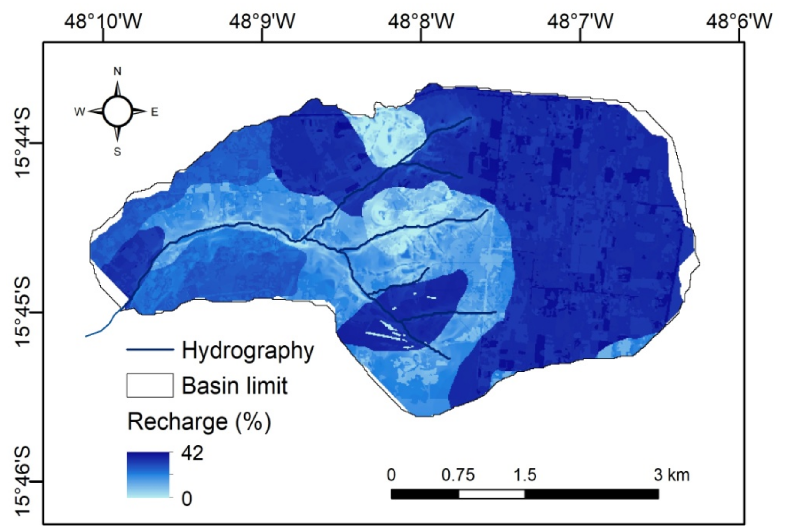
  • Among the four methods applied, only hydrological modeling estimates the potential recharge rate accurately. For this method, the result was considered satisfactory, since the average value of 35% for the basin was also estimated by hydrological modeling in other studies for basins in the same biome and with similar physical characteristics. However, the recharge rates in the Cerrado biome may be greater than estimated, as the simulated drainage discharge was probably underestimated in some areas of the basin;
  • in terms of effective recharge, of the three applied methods, numerical modeling presented the most promising results because, unlike the Baseflow and WTE methods, the rates are simulated considering the hydrodynamic and physical behavior of the aquifer. According to this method, the average recharge rate in the basin was around 21% of the total rainfall;
  • the WTE method also simulated a plausible average effective recharge for the basin of around 29% of the annual precipitation (the average annual rate calculated from point estimates). The baseflow estimate of around 37% was considered overestimated and the parameter of the mathematical filter was arbitrary and needs adjustment. The 25% estimated in Santos [85] for the same study area was considered more reasonable;
  • the level of uncertainty for the estimated recharge rates was not measured but was considered high due to uncertainties in the conceptual models of the methods, the uncertainties of the parameters/data, and the limitations of the results;
  • in terms of the spatial distribution, the potential recharge map generated by hydrological modeling was considered consistent for combinations between Ferralsols and Cerrado vegetation cover in flatter areas. For the steepest areas with Cambisols, the consistency of the map should be verified by applying another method because, according to Santos [86], the result differs greatly from that obtained by applying SWAT under the same conditions;
  • for effective recharge, the spatial distribution generated by numerical modeling was considered more consistent than the map generated by interpolation of the point estimates of the WTE method. However, the prior imposition of recharge zones generated by the method limits and makes the calibration process difficult. An alternative to this is the integrated simulation of the vadose and saturated zone [47];
  • all methods applied require at least one type of data or parameter that is not easily available and is difficult to obtain or estimate, indicating two main obstacles: A lack of basic field data, and the difficulty to build conceptual models faithful to the actual configuration of the hydrological processes, notably regarding numerical modeling of the saturated zone;
  • the baseflow separation, WTE, and numerical modeling of the saturated zone methods could not have been applied in any area under the typical Cerrado biome conditions, for example, karst, as among the tested methods, only surface distributed hydrological modeling would be feasible to study the recharge process over most of the biome;
  • the monitoring intensified in space and time performed at the study area was essential to reaching the results presented. However, for most situations, this intensity of survey would be unfeasible due to the resources required. In this sense, an alternative would be to implement a network of experimental basins, aiming to find an adequate level of representativity for the heterogeneity of the Cerrado biome. In such basins, highly detailed studies could be executed using fewer resources, and the results could be regionalized and transposed to similar areas;
  • despite the limitations of the alternative approach proposed—inverse modeling with previous mapping of recharge areas via multicriteria method—the result obtained is relevant because the mean effective recharge estimated for the basin was comparable to estimates obtained by other studies for the Cerrado areas, and the spatial distribution of the previously mapped areas were coherent considering the physical behavior and the interaction between environmental factors. The calibrated model could be refined and applied to the simulation of challenging scenarios for water resources integrated management, such as climate change, water use permits, and overexploitation;
  • the divergences between methods applied do not invalidate their results or applicability, since these differences are common and expected, considering the premise and simplifications inherent to each approach. As the actual measured values of the recharge in the area are not available, all of the results we obtained may undergo future evaluation through comparison with other methods, for example, using the lysimeter and chemical tracer methods, to further assess the groundwater recharge process in the Brazilian Cerrado biome.

Author Contributions

Conceptualization, R.M.d.S., S.K.; methodology, R.M.d.S., S.K.; validation, B.E.T., and D.L.d.A.; resources, S.K.; writing—original draft preparation, R.M.d.S.; writing—review and editing, R.M.d.S., S.K., B.E.T., and D.L.d.A.; supervision, S.K.; funding acquisition, S.K. All authors have read and agreed to the published version of the manuscript.

Funding

This research was funded by Conselho Nacional de Desenvolvimento Científico e Tecnológico (CNPq), Coordenação de Aperfeiçoamento de Pessoal de Nível Superior (CAPES) and Fundação de Apoio à Pesquisa do Distrito Federal (FAP-DF), for the PhD scholarship and further financial support granted to execute the work.

Institutional Review Board Statement

Not applicable.

Informed Consent Statement

Not applicable.

Data Availability Statement

The data presented in this study are available on request from the corresponding author. The data is not publicly available due to rules from secondary institutions that provided data to the study.

Acknowledgments

The authors thank the public worker Irioman Junior for the support on field activities and Empresa Brasileira de Pesquisa Agropecuária (EMBRAPA) Cerrados for providing the meteorological data.

Conflicts of Interest

The authors declare no conflict of interest.

References

  1. Xie, Y.; Cook, P.G.; Simmons, C.T.; Partington, D.; Crosbie, R.; Batelaan, O. Uncertainty of groundwater recharge estimated from a water and energy balance model. J. Hydrol. 2018, 561, 1081–1093. [Google Scholar] [CrossRef] [Green Version]
  2. Hund, S.V.; Allen, D.M.; Morillas, L.; Johnson, M.S. Groundwater recharge indicator as tool for decision makers to increase socio-hydrological resilience to seasonal drought. J. Hydrol. 2018, 563, 1119–1134. [Google Scholar] [CrossRef]
  3. Lamichhane, S.; Shakya, N.M. Alteration of groundwater recharge areas due to land use/cover change in Kathmandu Valley, Nepal. J. Hydrol. Reg. Stud. 2019, 26, 100635. [Google Scholar] [CrossRef]
  4. Bhanja, S.N.; Mukherjee, A.; Ramaswamy, R.; Scanlon, B.R.; Malakar, P.; Verma, S. Long-term groundwater recharge rates across India by in situ measurements. Hydrol. Earth Syst. Sci. Discuss. 2018, 1–19. [Google Scholar] [CrossRef] [Green Version]
  5. Hu, W.; Wang, Y.Q.; Li, H.J.; Huang, M.B.; Hou, M.T.; Li, Z.; She, D.L.; Si, B.C. Dominant role of climate in determining spatio-temporal distribution of potential groundwater recharge at a regional scale. J. Hydrol. 2019, 578. [Google Scholar] [CrossRef]
  6. Huang, X.; Gao, L.; Crosbie, R.S.; Zhang, N.; Fu, G.; Doble, R. Groundwater recharge prediction using linear regression, multi-layer perception network, and deep learning. Water 2019, 11, 1879. [Google Scholar] [CrossRef] [Green Version]
  7. Ashaolu, E.D.; Olorunfemi, J.F.; PaulIfabiy, I.; Abdollahi, K.; Batelaan, O. Spatial and temporal recharge estimation of the basement complex in Nigeria, West Africa. J. Hydrol. Reg. Stud. 2020, 27, 100658. [Google Scholar] [CrossRef]
  8. Mattos, T.S.; de Oliveira, P.T.S.; Lucas, M.C.; Wendland, E. Groundwater recharge decrease replacing pasture by Eucalyptus plantation. Water 2019, 11, 1213. [Google Scholar] [CrossRef] [Green Version]
  9. Watson, A.; Eilers, A.; Miller, J.A. Recharge estimation using cmb and environmental isotopes in the verlorenvlei estuarine system, south africa and implications for groundwater sustainability in a semi-arid agricultural region. Water 2020, 12, 1362. [Google Scholar] [CrossRef]
  10. Yihdego, Y.; Khalil, A. Groundwater resources assessment and impact analysis using a conceptual water balance model and time series data analysis: Case of decision making tool. Hydrology 2017, 4, 25. [Google Scholar] [CrossRef] [Green Version]
  11. Zhang, Y.; Liu, S.; Cheng, F.; Shen, Z. WetSpass-based study of the effects of urbanization on the water balance components at regional and quadrat scales in Beijing, China. Water 2017, 10, 5. [Google Scholar] [CrossRef] [Green Version]
  12. Rukundo, E.; Doğan, A. Dominant influencing factors of groundwater recharge spatial patterns in Ergene river catchment, Turkey. Water 2019, 11, 653. [Google Scholar] [CrossRef] [Green Version]
  13. Tenenwurcel, M.A.; de Moura, M.S.; da Costa, A.M.; Mota, P.K.; Viana, J.H.M.; Fernandes, L.F.S.; Pacheco, F.A.L. An improved model for the evaluation of groundwater recharge based on the concept of conservative use potential: A study in the river Pandeiros Watershed, Minas Gerais, Brazil. Water 2020, 12, 1001. [Google Scholar] [CrossRef] [Green Version]
  14. Zhu, R.; Croke, B.F.W.; Jakeman, A.J. Diffuse groundwater recharge estimation confronting hydrological modelling uncertainty. J. Hydrol. 2020, 584, 124642. [Google Scholar] [CrossRef]
  15. Santos, R.M. Recarga de águas Subterrâneas em Ambiente de Cerrado: Estudo com Base em Modelagem Numérica e Simulação Hidrológica em uma Bacia Experimental (Distrito Federal); Universidade de Brasília: Brasília, Brazil, 2012. [Google Scholar]
  16. Gonçalves, R.D.; Teramoto, E.H.; Chang, H.K. Regional Groundwater Modeling of the Guarani Aquifer System. Water 2020, 12, 2323. [Google Scholar] [CrossRef]
  17. Oliveira, P.T.S.; Wendland, E.; Nearing, M.A.; Scott, R.L.; Rosolem, R.; Da Rocha, H.R. The water balance components of undisturbed tropical woodlands in the Brazilian cerrado. Hydrol. Earth Syst. Sci. 2015, 19, 2899–2910. [Google Scholar] [CrossRef] [Green Version]
  18. de Almeida Salles, L.; Lima, J.E.F.W.; Roig, H.L.; Malaquias, J.V. Environmental factors and groundwater behavior in an agricultural experimental basin of the Brazilian central plateau. Appl. Geogr. 2018, 94, 272–281. [Google Scholar] [CrossRef]
  19. Lima, J.E.F.W. Situação e perspectivas sobre as águas do cerrado. Cienc. Cult. 2011, 63, 27–29. [Google Scholar] [CrossRef] [Green Version]
  20. Cambraia Neto, A.J.; Rodrigues, L.N. Evaluation of groundwater recharge estimation methods in a watershed in the Brazilian Savannah. Environ. Earth Sci. 2020, 79, 1–14. [Google Scholar] [CrossRef]
  21. Seraphim, A.P.A.C.C. Texto para Discussão (TD)—n. 55—Relações Entre as áreas de Recarga dos Aquíferos e áreas Destinadas à Urbanização: Estudo dos Padrões de Ocupação do solo da Unidade Hidrográfica do Lago Paranoá—DF; Universidade de Brasília: Brasília, Brazil, 2018. [Google Scholar]
  22. Carvalho, F.; Scopel, I. Escoamento superficial e recarga d’água subterrânea em diferentes usos do solo na microbacia do córrego do queixada. Rev. Caminhos Geogr. 2018, 19, 133–145. [Google Scholar] [CrossRef]
  23. Joshi, S.K.; Rai, S.P.; Sinha, R.; Gupta, S.; Densmore, A.L.; Rawat, Y.S.; Shekhar, S. Tracing groundwater recharge sources in the northwestern Indian alluvial aquifer using water isotopes (δ18O, δ2H and 3H). J. Hydrol. 2018, 559, 835–847. [Google Scholar] [CrossRef]
  24. Lentswe, G.B.; Molwalefhe, L. Delineation of potential groundwater recharge zones using analytic hierarchy process-guided GIS in the semi-arid Motloutse watershed, eastern Botswana. J. Hydrol. Reg. Stud. 2020, 28, 100674. [Google Scholar] [CrossRef]
  25. de Andrade Pinto, E.J.; Santo Lima, J.D.; Davis, E.G.; da Silva, A.J.; de Oliveira Dantas, C.E.; de Oliveira Candido, M.; Palmier, L.R.; de Almeida Monte-Mor, R.C. Estimativa Da Recarga Natural Do Aquífero Livre De Uma Sub-Bacia Da Bacia Representativa De Juatuba ( MG ) Aplicando O Método Da Variação Dos Níveis D’ Água (VNA). Available online: https://aguassubterraneas.abas.org/asubterraneas/article/view/23095 (accessed on 7 April 2020).
  26. Lousada, E.O.; Campos, J.E.G. Estudos isotópicos em águas subterrâneas do Distrito Federal: Subsídios ao modelo conceitual de fluxo. Rev. Bras. Geociências 2011, 41, 355–365. [Google Scholar] [CrossRef] [Green Version]
  27. Agência Nacional de Águas. Estratégias de Manejo Sustentável dos Sistemas Aquíferos Urucuia e Areado e Conclusões. Relatório Final; Agência Nacional de Águas: Brasília, Brazil, 2017; Volume 3. [Google Scholar]
  28. Ramires, T.; Manzione, R.L. Groundwater recharge estimation using water budget method for Bauru Aquifer system in a Cerrado environmental protection area. Appl. Res. Agrotechnol. 2019, 12, 25–36. [Google Scholar] [CrossRef]
  29. Gonçalves, V.F.M.; Manzione, R.L. Estimativa da recarga das águas subterrâneas no Sistema Aquífero Bauru (SAB). Geo UERJ 2019, 35, 2–19. [Google Scholar] [CrossRef]
  30. Silva, C.O.F. Modelagem Espacial da Recarga de águas Subterrâneas sob Diferentes Usos e Coberturas da Terra; Universidade Estadual Paulista: São Paulo, Brazil, 2019. [Google Scholar]
  31. Scanlon, B.R.; Healy, R.W.; Cook, P.G. Choosing appropriate techniques for quantifying groundwater recharge. Hydrogeol. J. 2002, 10, 18–39. [Google Scholar] [CrossRef]
  32. Lacombe, G.; Douangsavanh, S.; Vongphachanh, S.; Pavelic, P. Regional assessment of groundwater recharge in the lower mekong basin. Hydrology 2017, 4, 60. [Google Scholar] [CrossRef] [Green Version]
  33. Salem, A.; Dezso, J.; El-Rawy, M.; Lóczy, D. Hydrological modeling to assess the efficiency of groundwater replenishment through natural reservoirs in the Hungarian drava river floodplain. Water 2020, 12, 250. [Google Scholar] [CrossRef] [Green Version]
  34. Walker, D.; Parkin, G.; Schmitter, P.; Gowing, J.; Tilahun, S.A.; Haile, A.T.; Yimam, A.Y. Insights from a multi-method recharge estimation comparison study. Groundwater 2019, 57, 245–258. [Google Scholar] [CrossRef] [Green Version]
  35. Xu, Y.; Beekman, H.E. Review: Groundwater recharge estimation in arid and semi-arid southern Africa. Hydrogeol. J. 2019, 27, 929–943. [Google Scholar] [CrossRef]
  36. Neukum, C.; Azzam, R. Impact of climate change on groundwater recharge in a small catchment in the Black Forest, Germany. Hydrogeol. J. 2012, 20, 547–560. [Google Scholar] [CrossRef]
  37. Wiebe, A.J.; Rudolph, D.L. On the sensitivity of modelled groundwater recharge estimates to rain gauge network scale. J. Hydrol. 2020, 585, 124741. [Google Scholar] [CrossRef]
  38. Staśko, S.; Tarka, R.; Olichwer, T. Groundwater recharge evaluation based on the infiltration method. Groundw. Qual. Sustain. 2012, 189–198. [Google Scholar] [CrossRef]
  39. Tarka, R.; Olichwer, T.; Staośko, S. Evaluation of groundwater recharge in Poland using the infiltration coefficient method. Geol. Q. 2016, 61, 384–395. [Google Scholar] [CrossRef] [Green Version]
  40. Siva Prasad, Y.; Venkateswara Rao, B. Groundwater recharge estimation studies in a khondalitic terrain of India. Appl. Water Sci. 2018, 8, 1–9. [Google Scholar] [CrossRef] [Green Version]
  41. Yang, W.; Xiao, C.; Liang, X. Extraction method of baseflow recession segments based on second-order derivative of streamflow and comparison with four conventional methods. Water 2020, 12, 1953. [Google Scholar] [CrossRef]
  42. Lovett, A.; Gordon, D.; Srinivasan, M.S.; White, P. Fabrication and installation of an arable lysimeter for measuring groundwater recharge in New Zealand. Presented at the 17th Gumpensteiner Lysimetertagung: LysimeterForschung-Möglichkeiten und Grenzen Lysimeter research - options and limits, Raumberg-Gumpenstein, Austria, 9–10 May 2017. CAB Direct. Available online: https://www.cabdirect.org/cabdirect/abstract/20183101856 (accessed on 10 March 2020).
  43. Kohfahl, C.; Molano-Leno, L.; Martínez, G.; Vanderlinden, K.; Guardiola-Albert, C.; Moreno, L. Determining groundwater recharge and vapor flow in dune sediments using a weighable precision meteo lysimeter. Sci. Total Environ. 2019, 656, 550–557. [Google Scholar] [CrossRef]
  44. Huo, S.; Jin, M.; Liang, X.; Li, X.; Hao, H. Estimating impacts of water-table depth on groundwater evaporation and recharge using lysimeter measurement data and bromide tracer. Hydrogeol. J. 2020, 28, 955–971. [Google Scholar] [CrossRef]
  45. Collenteur, R.; Bakker, M.; Klammler, G.; Birk, S. Estimating groundwater recharge from groundwater levels using non-linear transfer function noise models and comparison to lysimeter data. Hydrol. Earth Syst. Sci. Discuss. 2020, 1–30. [Google Scholar] [CrossRef]
  46. Carvalho, V.E.C.; Rezende, K.S.; Paes, B.S.T.; Betim, L.S.; Marques, E.A.G. Estimativa da recarga em uma sub-bacia hidrográfica rural através do método da Variação do Nível d-Água (VNA). Rev. Bras. Recur. Hídricos 2014, 19, 271–280. [Google Scholar] [CrossRef]
  47. Araujo, D.L. Avaliação dos Impactos da Explotação de águas Subterrâneas na Bacia do Ribeirão Rodeador por Meio de Simulação Integrada Entre os Modelos SWAT e MODFLOW; Universidade de Brasília: Brasília, Brazil, 2018. [Google Scholar]
  48. Salem, A.; Dezso, J.; El-Rawy, M. Assessment of Groundwater Recharge, Evaporation, and Runoff in the Drava Basin in Hungary with the WetSpass Model. Hydrology 2019, 6, 23. [Google Scholar] [CrossRef] [Green Version]
  49. Singh, A.; Panda, S.N.; Uzokwe, V.N.E.; Krause, P. An assessment of groundwater recharge estimation techniques for sustainable resource management. Groundw. Sustain. Dev. 2019, 9. [Google Scholar] [CrossRef]
  50. Yihdego, Y.; Danis, C.; Paffard, A. Why is the Groundwater Level Rising? A Case Study Using HARTT to Simulate Groundwater Level Dynamic. Water Environ. Res. 2017, 89, 2142–2152. [Google Scholar] [CrossRef]
  51. Cartwright, I.; Cendón, D.; Currell, M.; Meredith, K. A review of radioactive isotopes and other residence time tracers in understanding groundwater recharge: Possibilities, challenges, and limitations. J. Hydrol. 2017, 555, 797–811. [Google Scholar] [CrossRef]
  52. Richards, L.A.; Magnone, D.; Boyce, A.J.; Casanueva-Marenco, M.J.; van Dongen, B.E.; Ballentine, C.J.; Polya, D.A. Delineating sources of groundwater recharge in an arsenic-affected Holocene aquifer in Cambodia using stable isotope-based mixing models. J. Hydrol. 2018, 557, 321–334. [Google Scholar] [CrossRef] [Green Version]
  53. Li, Z.; Jasechko, S.; Si, B. Uncertainties in tritium mass balance models for groundwater recharge estimation. J. Hydrol. 2019, 571, 150–158. [Google Scholar] [CrossRef]
  54. Parlov, J.; Kovač, Z.; Nakić, Z.; Barešić, J. Using water stable isotopes for identifying groundwater recharge sources of the unconfined alluvial Zagreb aquifer (Croatia). Water 2019, 11, 2177. [Google Scholar] [CrossRef] [Green Version]
  55. Ahmed, I.M.; Jalludin, M.; Razack, M. Hydrochemical and isotopic assessment of groundwater in the Goda mountains range system. Republic of Djibouti (horn of Africa). Water 2020, 12, 2004. [Google Scholar] [CrossRef]
  56. Gonçalves, R.D.; Teramoto, E.H.; Engelbrecht, B.Z.; Alfaro Soto, M.A.; Chang, H.K.; van Genuchten, M.T. Quasi-Saturated Layer: Implications for Estimating Recharge and Groundwater Modeling. Groundwater 2019, 58, 432–440. [Google Scholar] [CrossRef]
  57. Ouyang, Y.; Jin, W.; Grace, J.M.; Obalum, S.E.; Zipperer, W.C.; Huang, X. Estimating impact of forest land on groundwater recharge in a humid subtropical watershed of the Lower Mississippi River Alluvial Valley. J. Hydrol. Reg. Stud. 2019, 26, 100631. [Google Scholar] [CrossRef]
  58. Petronici, F.; Pujades, E.; Jurado, A.; Marcaccio, M.; Borgatti, L. Numerical modelling of the Mulino Delle Vene Aquifer (Northern Italy) as a tool for predicting the hydrogeological system behavior under different recharge conditions. Water 2019, 11, 2505. [Google Scholar] [CrossRef] [Green Version]
  59. Bizhanimanzar, M.; Leconte, R.; Nuth, M. Catchment-Scale Integrated Surface Water-Groundwater Hydrologic Modelling Using. Water 2020, 12, 363. [Google Scholar] [CrossRef] [Green Version]
  60. Yihdego, Y.; Danis, C.; Paffard, A. Groundwater engineering in an environmentally sensitive urban area: Assessment, landuse change/infrastructure impacts and mitigation measures. Hydrology 2017, 4, 37. [Google Scholar] [CrossRef] [Green Version]
  61. Monte-Mor, R.C.A.; Palmier, L.R.; Pinto, E.J.A.; Lima, J.E.S. Estabilidade temporal da distribuição espacial da umidade do solo em uma bacia intermitente no semiárido de Minas Gerais. Rev. Bras. Recur. Hidricos 2012, 17, 101–113. [Google Scholar] [CrossRef]
  62. Martins, É.D.S.; Reatto, A.; Carvalho, O.A., Jr.; Guimarães, R.F. Unidades de Paisagem do Distrito Federal, Escala 1: 100.000; Embrapa Cerrados: Planaltina-Distrito Federal, Brazil, 2004. [Google Scholar]
  63. Reatto, A.; Martins, É.D.S.; Cardoso, E.A.; Spera, S.T.; Carvalho, O.A., Jr.; De Silva, A.V.; Farias, M.F.R. Levantamento de Reconhecimento de Solos de Alta Intensidade do Alto Curso do rio Descoberto; Embrapa Cerrados: Planaltina-Distrito Federal, Brazil, 2003. [Google Scholar]
  64. CPRM; Embrapa. Zoneamento Ecológico-Econômico da Região Integrada de Desenvolvimento do Distrito Federal e Entorno: Fase I; Ministério do Meio Ambiente: Rio de Janeiro, Brazil, 2003; Volume 1. [Google Scholar]
  65. Al-aboodi, A.H.; Ibrahim, H.T.; Ibrahim, N. Estimation of Groundwater Recharge in Safwan-Zubair Area, South of Iraq, Using Water Balance and Inverse Modeling Methods. Int. J. Civ. Eng. Technol. 2019, 10, 202–210. [Google Scholar]
  66. Santos, R.M.; Koide, S. Avaliação da recarga de águas subterrâneas em ambiente de cerrado com base em modelagem numérica do fluxo em meio poroso saturado. Rev. Bras. Recur. Hidricos 2016, 21, 451–465. [Google Scholar] [CrossRef]
  67. Tucci, C.E.M. Modelos Hidrológicos, 1st ed.; Editora UFRGS: Porto Alegre, Brazil, 2005. [Google Scholar]
  68. Eiten, G. The Cerrado Vegetation of Brazil. Bot. Rev. 1972, 38, 201–341. [Google Scholar] [CrossRef]
  69. Canadell, J.; Jackson, R.B.; Mooney, H.A.; Sala, O.E.; Schulze, E.D. Maximum rooting depth of vegetation tyoes at the global scale. Oecologia 1996, 108, 583–595. [Google Scholar] [CrossRef]
  70. Ferreira, M.D.N. Distribuição Radicular e Consumo de água de Goiabeira (Psidium guajava L.) Irrigada por Microaspersão em Petrolina-PE; Universidade de São Paulo: São Paulo, Brazil, 2004. [Google Scholar]
  71. Silvério-Júnior, J. Aplicação do método Analytic Hierarchy Process na Avaliação de Indicadores Setoriais de Arranjos Produtivos Locais: Caso do APL de Madeira e Móveis de Paragominas—PA; Universidade Católica de Brasília: Brasília, Brazil, 2006. [Google Scholar]
  72. Vargas, R.V. Using the analytic hierarchy process (ahp) to select and prioritize projects in a portfolio. In Proceedings of the PMI Global Congress 2010, Washington, DC, USA, 9–12 October 2010; Project Management Institute:: Washington, DC, USA, 2010. [Google Scholar]
  73. Schlumberger Water Services. Visual MODFLOW V.2.8.2 User’s Manual for Professional Applications in Three-Dimensional Groundwater Flow and Contaminant Transport Modeling; Schlumberger: Kitchener, ON, Canada, 2000. [Google Scholar]
  74. Hill, M.C.; Tiedman, C.R. Effective Groundwater Model Calibration; Willey: Hoboken, NJ, USA, 2007. [Google Scholar]
  75. Beven, K.; Freer, J. Equifinality, data assimilation, and uncertainty estimation in mechanistic modelling of complex environmental systems using the GLUE methodology. J. Hydrol. 2001, 249, 11–29. [Google Scholar] [CrossRef]
  76. Waterloo Hydrogeologic Inc. User’s Manual for WinPEST; Waterloo Hydrogeologic: Waterloo, ON, Canada, 1999. [Google Scholar]
  77. Liu, Y.B.; DeSmedt, F. WetSpa Extension, A GIS-Based Hydrologic Model for Flood Prediction and Watershed Management Documentation and User Manual; Vrije Universiteit Brussel: Brussel, Belgium, 2004. [Google Scholar]
  78. Bahremand, A.; De Smedt, F.; Corluy, J.; Liu, Y.B.; Poórová, J.; Velcická, L.; Kunikova, E. Application of WetSpa model for assessing land use impacts on floods in the Margecany-Hornad watershed, Slovakia. Water Sci. Technol. 2006, 53, 37–45. [Google Scholar] [CrossRef]
  79. Healy, R.W.; Cook, P.G. Using groundwater levels to estimate recharge. Hydrogeol. J. 2002, 10, 91–109. [Google Scholar] [CrossRef]
  80. Bortolin, T.A.; Reginato, P.A.R.; Presotto, M.A.; Schneider, V.E. Estimativas de recarga aquífera com uso de filtros digitais em sub-bacias hidrográficas do Sistema Aquífero Serra Geral no estado do Rio Grande do Sul. Sci. Ind. 2018, 6, 21–30. [Google Scholar] [CrossRef] [Green Version]
  81. Wittenberg, H.; Sivapalan, M. Watershed groundwater balance estimation using streamflow recession analysis and baseflow separation. J. Hydrol. 1999, 219, 20–33. [Google Scholar] [CrossRef]
  82. Safari, A.; De Smedt, F.; Moreda, F. WetSpa model application in the Distributed Model Intercomparison Project (DMIP2). J. Hydrol. 2012, 418–419, 78–89. [Google Scholar] [CrossRef]
  83. Souza, E.; Pontes, L.M.; Fernandes Filho, E.I.; Schaefer, C.E.G.R.; Santos, E.E. Spatial and temporal potential groundwater recharge: The case of the doce river basin, Brazil. Rev. Bras. Cienc. Solo 2019, 43, 1–27. [Google Scholar] [CrossRef] [Green Version]
  84. Agência Nacional de Águas. Estudos Hidrogeológicos e de Vulnerabilidade do Sistema Aquífero Urucuia e Proposição de Modelo de Gestão Integrada Compartilhada: Resumo Executivo; Agência Nacional de Águas: Brasília, Brazil, 2017; p. 100. [Google Scholar]
  85. Santos, M.S. Determinação de Escoamentos Mínimos e Separação de Escoamentos de Base na Bacia do Rio Descoberto; Universidade de Brasília: Brasília, Brazil, 2007. [Google Scholar]
  86. dos Santos, R.M.; Koide, S.; de Araujo, D.L.; Távora, B.E. Abacus to predict groundwater recharge at non-instrumented hydrographic basins. Water 2020, 12, 3090. [Google Scholar] [CrossRef]
Figure 1. Location of the study area.
Water 13 00020 g001
Figure 2. Steps of the numerical modelling method. (A)Items of the conceptual hydrogeological model; (B) steps of the numerical model implementation; (C) database partition between modeling steps; (D)steps of the calibration process; (E) calibration process evaluation; and (F) recharge estimation by inverse modelling [15,66].
Water 13 00020 g002
Figure 3. Conceptual model of the groundwater recharge and flow in the numerical model.perspective and cross section view.
Water 13 00020 g003
Figure 4. Hydrological processes and WETSPA (water and energy transfer between soils, plants, and atmosphere) model structure [77].
Water 13 00020 g004
Figure 5. Spatial distribution of the numerical model parameters Ksat (saturated hydraulic conductivity) and Sy (specific yield coefficient). (A,C) Average values of point slug and pumping tests estimates for the first layer; (B,D) calibrated values for the second layer.
Water 13 00020 g005
Figure 6. Observed versus simulated piezometric heads for numerical modeling steps of calibration (A), verification (B), and inverse modeling (C).
Water 13 00020 g006
Figure 7. Measured versus modeled drainage discharge for the calibration (A), verification (B), and inverse modeling (C).
Water 13 00020 g007
Figure 8. Estimated spatial distribution of effective groundwater recharge in the study area based on numerical modeling (% annual precipitation).
Water 13 00020 g008
Figure 9. Measured versus modeled discharge (calibration).
Water 13 00020 g009
Figure 10. Measured versus modeled discharge (verification).
Water 13 00020 g010
Figure 11. Estimated spatial distribution of potential groundwater recharge: Distributed hydrological modeling.
Water 13 00020 g011
Figure 12. Estimated spatial distribution of effective groundwater recharge in the study area for the hydrological year 2008/2009, according to the WTE method.
Water 13 00020 g012
Figure 13. Hydrographof surface flow and baseflow for 2007/2008.
Water 13 00020 g013
Figure 14. Hydrograph of surface flow and baseflow for 2008/2009.
Water 13 00020 g014
Table 1. WETSPA local and global parameters.
Local Parameters
Hydraulic conductivityFunction of soil texture class.
Porosity
Field capacity
Wilting pointFunction of soil texture class.
Residual moisture content
Pore size distribution index
Interception capability (minimum and maximum)Function of land use and cover.
Root system depth
Manning coefficient
Percentage of vegetation cover
Leaf area index
Surface runoff coefficientFunction of slope, soil texture class, and land use and cover.
Depression storage capacityFunction of slope, soil texture class, and land use and cover.
Global Parameters
Coefficient to correct potential evapotranspiration (Kep)Used when the evapotranspiration station is located in a site with physical characteristics different from the area simulated.
Scale factor to calculate subsurface flow (Ki)Preferential pathways affect subsurface flow. Since WETSPA
considers the soil a homogeneous matrix, this parameter was used to compensate for the negative effects of such simplification.
Aquifer recession coefficient (Kg)Reflects the aquifer storage pattern in the basin. It can be
estimated from river monitoring data or calibrated, comparing observed and simulated flows, for the dry season.
Aquifer initial storage (G0)Used to compensate the effects of losses in the aquifer through deep percolation. It can be calibrated by comparing observed and simulated hydrographs, in the low flows of the initial simulation period (mm).
Aquifer maximum storage (Gmax)Aquifer maximum storage (mm), calibrated for low flows.
Coefficient to adjust effective precipitation equation for low intensity precipitation (K_run)Used to consider the effect of the precipitation intensity in
infiltration and generation of surface runoff.
Precipitation intensity to make “K_run” equals “1” (P_max)Threshold of precipitation intensity that causes a linear relation between surface runoff coefficient and current soil moisture
content. It can be estimated by calibration, comparing high
observed and simulated flows.
Table 2. Ksat and Sy for punctual field estimates and calibrated zones values.
Hydraulic Conductivity (m/day)
WellFilter Section Depth (m)Slug and Pumping Test EstimatesMean Values for ZonesCalibrated ValuesAbsolute
Difference (%)
01203.064.153.858
02204.044.153.858
031019.434.153.858
04154.074.153.858
0572.583.22 (layer 1)--
0663.583.22 (layer 1)--
07200.250.250.239
08126.646.641245
09200.910.911.5642
1073.543.22 (layer 1)--
11210.260.250.239
12150.260.250.239
13153.233.232.1550
1475.513.22 (layer 1)--
1590.070.250.239
16810.6210.625.00112
17810.6210.625.00112
18150.250.250.239
Specific Yield (DN)
0570.1200.120.138
09200.0120.0150.0133
1470.0890.89 (layer 1)--
17–168-0.20 (assigned based on the behavior of the medium sand)0.2210
Table 3. Sensitivity analysis results.
Local ParameterDischarge Variation (%) from Parameter
Increment of +20%
Discharge Variation (%) from Parameter
Increment of −20%
Hydraulic conductivity2−1
Porosity−49
Field capacity11
Wilting point4−2
Residual moisture content11
Pore size distribution index−37
Minimum interception capability11
Maximum interception capability11
Root system depth−35
Manning coefficient11
Percentage of vegetation cover11
Minimum leaf area index11
Maximum leaf area index11
Surface runoff coefficient11
Depression storage capacity11
Global ParameterDischarge Variation (%) from Parameter
Increment of +20%
Discharge Variation (%) from Parameter
Increment of –20%
Coefficient to correct potential
evapotranspiration (Kep)
−1717
Scale factor to calculate subsurface flow (Ki)11
Aquifer recession coefficient (Kg)5−5
Aquifer initial storage (G0)6−4
Aquifer maximum storage (Gmax)11
Coefficient to adjust effective
precipitation equation for low
intensity precipitation(K_run)
11
Precipitation intensity to make “K_run” equals “1” (P_max)11
Table 4. Calibrated global parameters.
Global
Parameter
Reference Values or Adjustment Strategy Calibrated Value
Kep (DN)1.000.660
Ki (DN)1.00–10 (calibrated from the measured and simulated values of the
recessive parts of the hydrograph)
2.753
Kg (DN)Calibrated from model performance for low flow values0.010
G0 (mm)Calibrated from initial discharge values614
Gmax (mm)Calibrated from model performance for low flow values1000
K_run (DN)Calibrated by simulated flow for small storms20.312
P_max (mm)Calibrated by simulated flow for small storms100
Table 5. Point recharge rate in the monitoring wells according to the water table elevation (WTE) method.
WellΔh(m) 2008/2009SyRecharge (mm)
012.300.1100253.00
022.000.1100220.00
032.900.1100319.00
042.600.1100286.00
052.500.1100275.00
064.10.1100451.00
077.100.0500355.00
0811.400.0500570.00
0918.000.0135243.00
105.100.0500255.00
1110.500.0135141.75
127.600.0500380.00
136.900.15501069.50
147.100.0500355.00
154.300.0500215.00
166.500.15501007.50
171.900.1550294.50
185.600.1550868.00
Average420.00 (29% of the total annual precipitation)
Table 6. Total annual effective recharge using baseflow separation.
Hydrological YearTotal Precipitation (mm)Recharge (mm/year)Recharge (% prec.)
2007/20081551469.5030.30
2008/20091589596.0537.44
Table 7. Recharge rates for the hydrological year 2008/2009 in the Capão Comprido watershed.
MethodRecharge 2008/2009 (mm)Recharge 2008/2009 (% Precipitation)
Hydrological modeling—WETSPA model51935 (potential recharge)
Numerical modeling32721 (effective recharge)
Water table elevation—WTE23015, from the map, and 29, average of the point estimates (effective recharge)
Baseflow: Mathematical filter59637 (25 in Santos [85]) (effective recharge)
Table 8. Methods and data required for groundwater recharge assessment. (Availability: 1 = frequent; 2 = regular; 3 = rare; Difficulty to obtain: A = low; B = medium; C = high).
MethodData/Parameters RequiredAvailabilityDifficulty to Obtain
Numerical modeling of water flow in saturated mediumSlopeAA
Geology and soil mappingBB
Time series of water table levelCC
Aquifer parameters (Ksat/Sy)CC
Aquifer structural characterization (thickness and layers)CC
Characterization of aquifer’s interaction with external environment (evapotranspiration and baseflow discharge)BB
Orbital imageryAA
Surface distributed hydrological modelingSlopeAA
Soil mappingBB
Land use/cover mappingAC
Soil’s hydrological characterizationBB
Root system depthAA
Manning coefficientAA
Leaf area indexAA
Surface runoff coefficientAA
Precipitation time seriesAB
Meteorological data time seriesAB
Total rive discharge time seriesAC
Baseflow separation using
mathematical filter
Flow temporal seriesAC
WTEPiezometric head time seriesCC
Sy estimationsCC
Publisher’s Note: MDPI stays neutral with regard to jurisdictional claims in published maps and institutional affiliations.

