Water Body Extraction from Sentinel-3 Image with Multiscale Spatiotemporal Super-Resolution Mapping


Abstract
1. Introduction
2. Methods
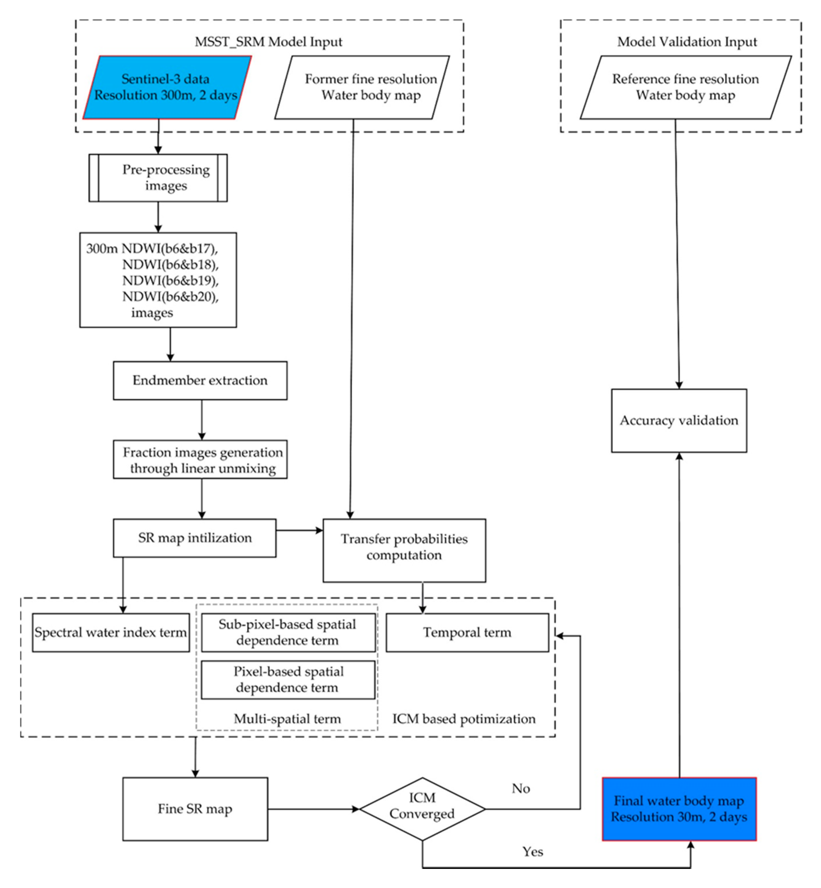
2.1. MSST_SRM
2.2. Spectral Water Index Term
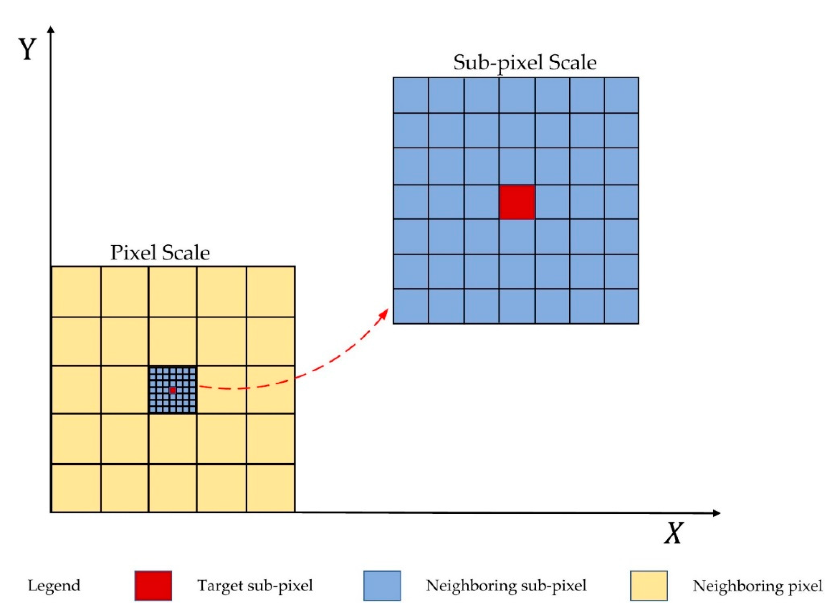
2.3. Multispatial Term
2.3.1. Subpixel-Based Spatial Dependence Term
2.3.2. Pixel-Based Spatial Dependence Term
2.4. Temporal Term
2.5. Implementation of MSST_SRM and Accuracy Validation
- (1)
- Initialize the input data and parameters and generate NDWI images by calculating Band 6 and Bands 17–20 from Sentinel-3 OLCI; set the proper values for scale factor z, key parameters α, , and β, and window sizes and .
- (2)
- Extract the endmember and then obtain fraction images by using the linear unmixing method. Then, initialize the SR map based on it.
- (3)
- Calculate the transition probability matrix.
- (4)
- Update the subpixel labels iteratively all over the whole image. The class label for each subpixel that contributes to the last iteration process is regarded as the final class label for this subpixel.
- (5)
- Stop the iteration after the algorithm converges or the iteration exceeds the setting number; otherwise, step 4 is repeated.
3. Experiments and Analysis
3.1. Experiment 1
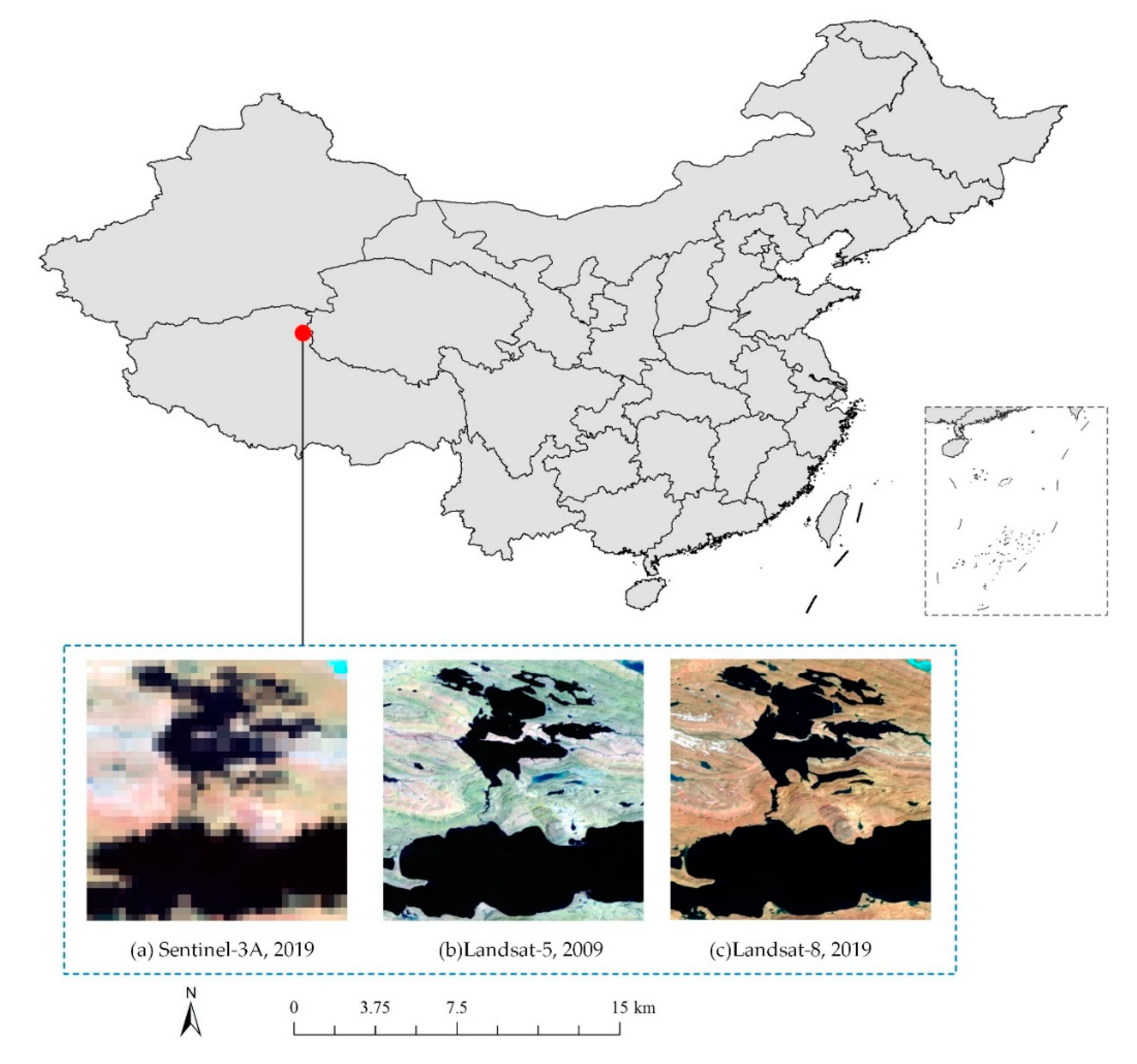
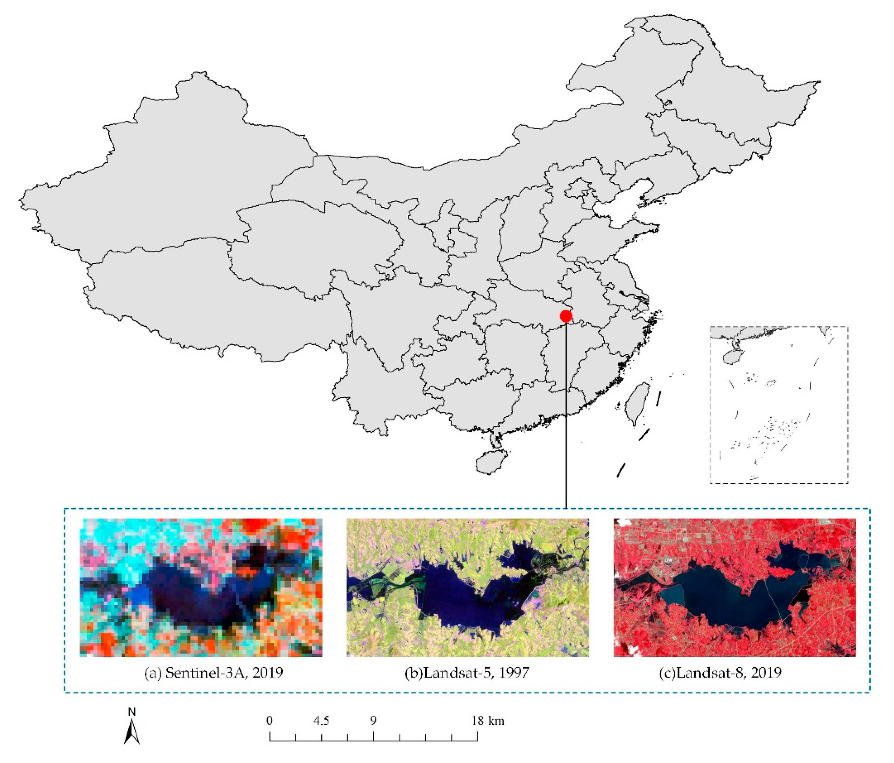
3.1.1. Study Area
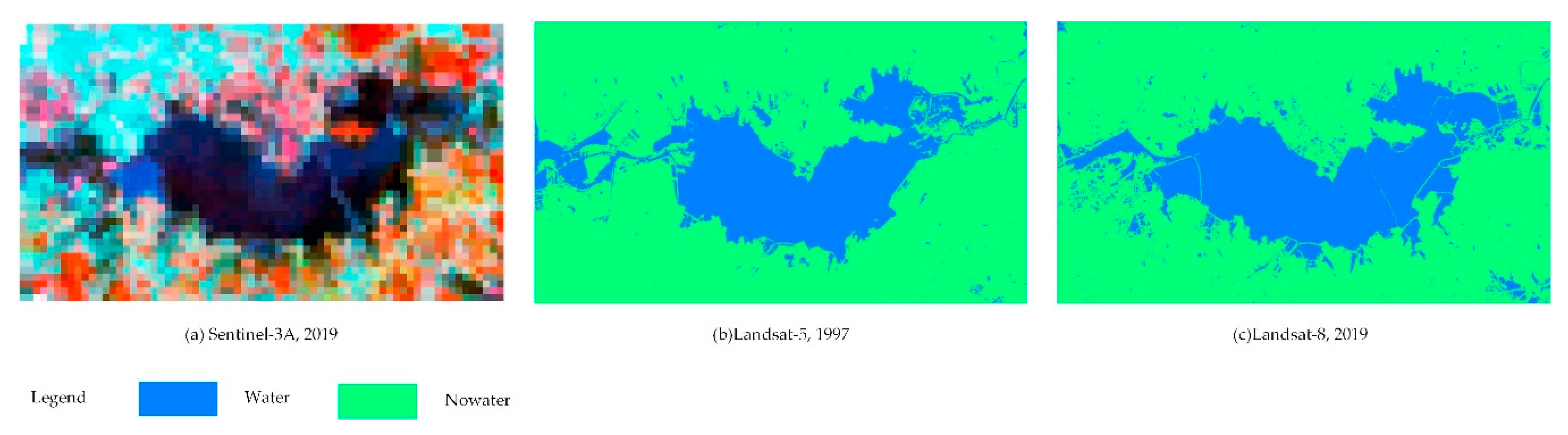
3.1.2. Data Sources and Preprocessing
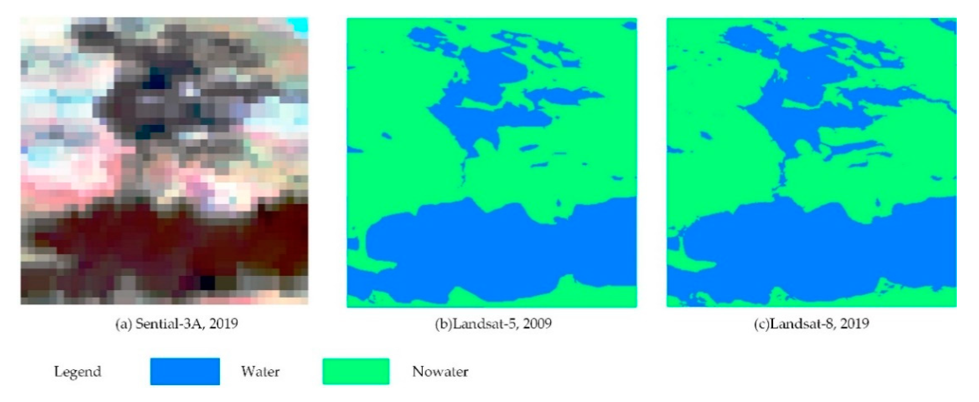
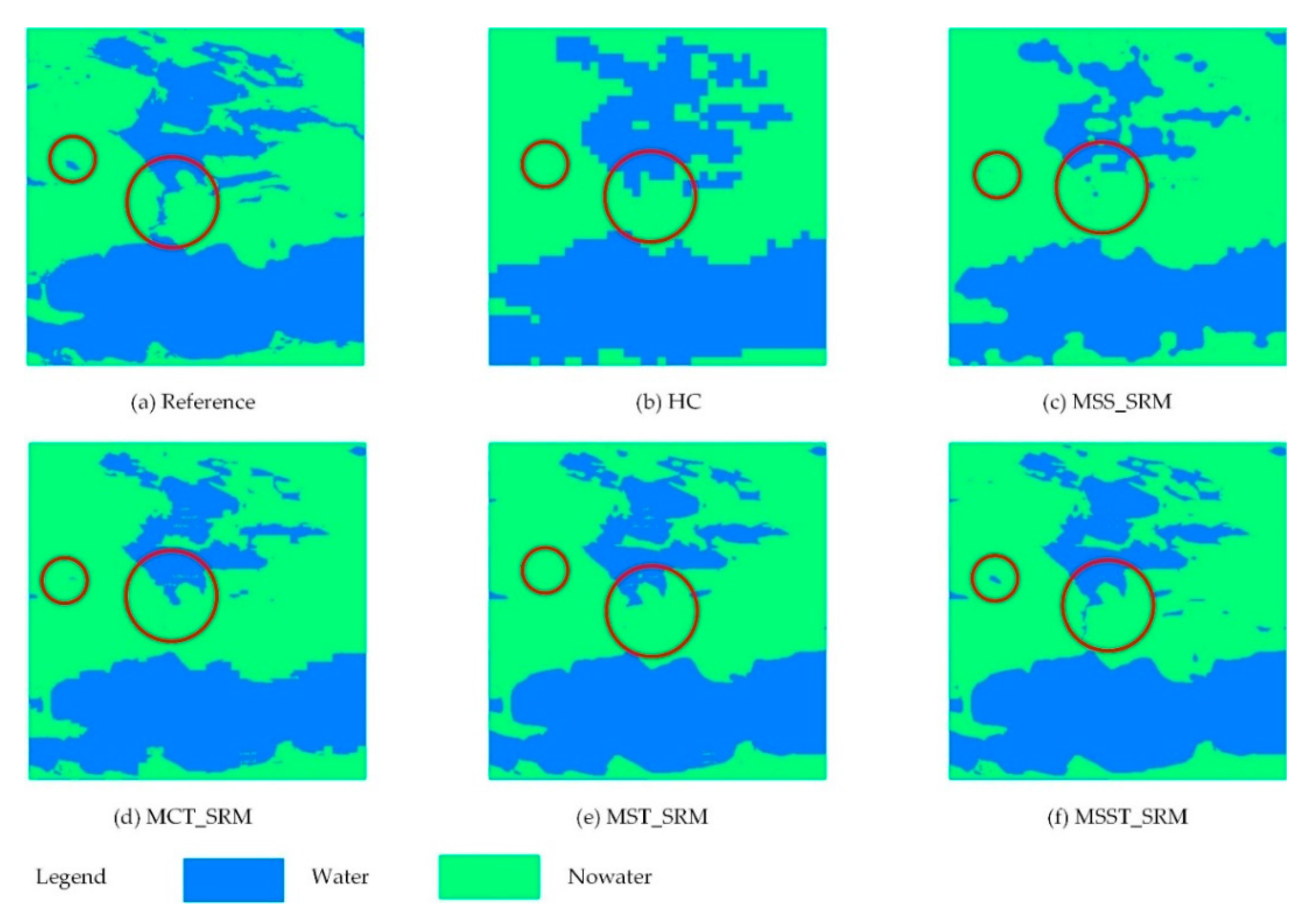
3.1.3. Results and Analysis
3.2. Experiment 2
3.2.1. Study Area
3.2.2. Data Sources and Preprocessing
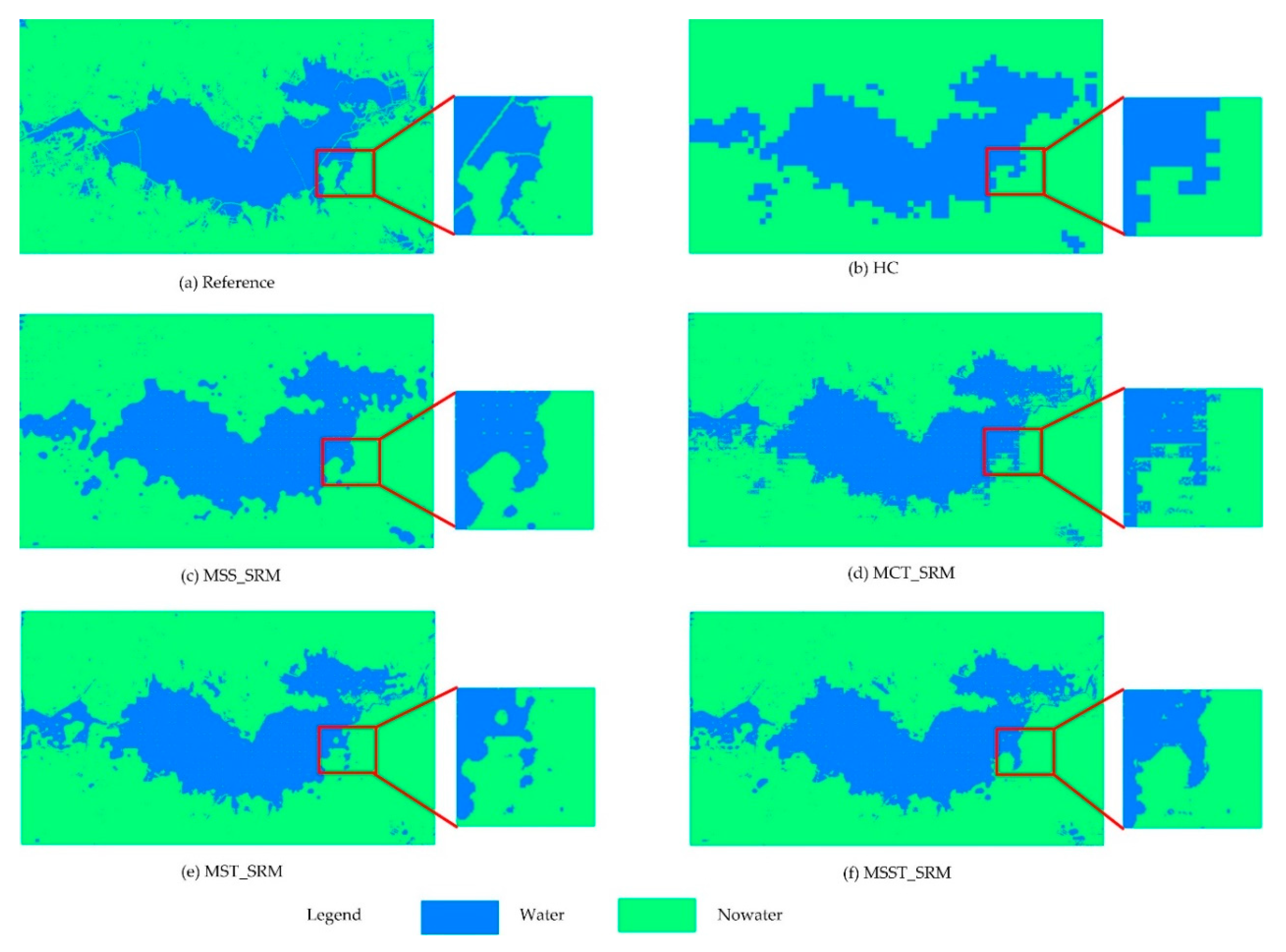
3.2.3. Results and Analysis
4. Discussion
4.1. Influences of Weighting Coefficients among Spectral, Multispatial, and Temporal Terms
4.2. Influences of Change Rate
5. Conclusions
Author Contributions
Funding
Conflicts of Interest
References
- Xu, L.; Abbaszadeh, P.; Moradkhani, H.; Chen, N.C.; Zhang, X. Continental drought monitoring using satellite soil moisture, data assimilation and an integrated drought index. Remote Sens. Environ. 2020, 250, 112028. [Google Scholar] [CrossRef]
- Tzanakakis, V.A.; Paranychianakis, N.V.; Angelakis, A.N. Water Supply and Water Scarcity. Water 2020, 12, 2347. [Google Scholar] [CrossRef]
- Xiong, L.; Deng, R.; Li, J.; Liu, X.; Qin, Y.; Liang, Y.; Liu, Y. Subpixel Surface Water Extraction (SSWE) Using Landsat 8 OLI Data. Water 2018, 10, 653. [Google Scholar] [CrossRef]
- Bioresita, F.; Puissant, A.; Stumpf, A.; Malet, J. A Method for Automatic and Rapid Mapping of Water Surfaces from Sentinel-1 Imagery. Remote Sens. 2018, 10, 217. [Google Scholar] [CrossRef]
- Davranche, A.; Lefebvre, G.; Poulin, B. Wetland monitoring using classification trees and SPOT-5 seasonal time series. Remote Sens. Environ. 2012, 114, 552–562. [Google Scholar] [CrossRef]
- Zhu, C.; Zhang, X.; Huang, Q. Four Decades of Estuarine Wetland Changes in the Yellow River Delta Based on Landsat Observations between 1973 and 2013. Water 2018, 10, 933. [Google Scholar] [CrossRef]
- Deus, D.; Gloaguen, R. Remote Sensing Analysis of Lake Dynamics in Semi-Arid Regions: Implication for Water Resource Management. Lake Manyara, East African Rift, Northern Tanzania. Water 2013, 5, 698–727. [Google Scholar] [CrossRef]
- Shi, L.; Ling, F.; Foody, G.M.; Chen, C.; Fang, S.; Li, X.; Zhang, Y.; Du, Y. Permanent disappearance and seasonal fluctuation of urban lake area in Wuhan, China monitored with long time series remotely sensed images from 1987 to 2016. Int. J. Remote Sens. 2019, 40, 8484–8505. [Google Scholar] [CrossRef]
- Kordelas, G.A.; Manakos, I.; Aragonés, D.; Díaz-Delgado, R.; Bustamante, J. Fast and Automatic Data-Driven Thresholding for Inundation Mapping with Sentinel-2 Data. Remote Sens. 2018, 10, 910. [Google Scholar] [CrossRef]
- Huang, X.; Wang, C.; Li, Z. Reconstructing flood inundation probability by enhancing near real-time imagery with real-time gauges and tweets. IEEE Trans. Geosci. Remote Sens. 2018, 56, 4691–4701. [Google Scholar] [CrossRef]
- Rishikeshan, C.A.; Ramesh, H. An automated mathematical morphology driven algorithm for water body extraction from remotely sensed images. ISPRS J. Photogramm. Remote Sens. 2018, 146, 11–21. [Google Scholar] [CrossRef]
- Jia, T.; Zhang, X.; Dong, R. Long-Term Spatial and Temporal Monitoring of Cyanobacteria Blooms Using MODIS on Google Earth Engine: A Case Study in Taihu Lake. Remote Sens. 2019, 11, 2269. [Google Scholar] [CrossRef]
- Dörnhöfer, K.; Oppelt, N. Remote sensing for lake research and monitoring—Recent advances. Ecol. Indic. 2016, 64, 105–122. [Google Scholar] [CrossRef]
- Ling, F.; Li, X.Y.; Foody, G.M.; Boyd, D.; Ge, Y.; Li, X.D.; Du, Y. Monitoring surface water area variations of reservoirs using daily MODIS images by exploring sub-pixel information. ISPRS J. Photogramm. Remote Sens. 2020, 168, 141–152. [Google Scholar] [CrossRef]
- Mcfeeters, S.K. The use of the normalized difference water index (NDWI) in the delineation of open water features. Int. J. Remote Sens. 1996, 17, 1425–1432. [Google Scholar] [CrossRef]
- Xu, H. Modification of normalised difference water index (NDWI) to enhance open water features in remotely sensed imagery. Int. J. Remote Sens. 2006, 27, 3025–3033. [Google Scholar] [CrossRef]
- Foody, G.M.; Cox, D.P. Sub-pixel land cover composition estimation using a linear mixture model and fuzzy membership functions. Int. J. Remote Sens. 1994, 15, 619–631. [Google Scholar] [CrossRef]
- Ling, F.; Boyd, D.; Ge, Y.; Foody, G.M.; Li, X.D.; Wang, L.H.; Zhang, Y.H.; Shi, L.D.; Shang, C.; Li, X.Y.; et al. Measuring River Wetted Width From Remotely Sensed Imagery at the Subpixel Scale With a Deep Convolutional Neural Network. Water Resour. Res. 2019, 55, 5631–5649. [Google Scholar] [CrossRef]
- Ling, F.; Li, X.D.; Xiao, F.; Du, Y. Super-Resolution Land Cover Mapping Using Spatial Regularization. IEEE Trans. Geosci. Remote Sens. 2014, 52, 4424–4439. [Google Scholar] [CrossRef]
- Chen, Y.; Ge, Y.; Jia, Y. Integrating object boundary in super-resolution land-cover mapping. IEEE J. Sel. Top. Appl. Earth Obs. Remote Sens. 2017, 10, 219–230. [Google Scholar] [CrossRef]
- Atkinson, P.M. Mapping sub-pixel vector boundaries from remotely sensed images. Innov. GIS 1997, 4, 166–180. [Google Scholar]
- Atkinson, P.M. Sub-pixel target mapping from soft-classified, remotely sensed imagery. Photogramm. Eng. Remote Sens. 2005, 71, 839–846. [Google Scholar] [CrossRef]
- Atkinson, P.M. Issues of uncertainty in super-resolution mapping and their implications for the design of an inter-comparison study. Int. J. Remote Sens. 2009, 30, 5293–5308. [Google Scholar] [CrossRef]
- Yang, X.; Xie, Z.; Ling, F.; Li, X.; Zhang, Y.; Zhong, M. Spatio-Temporal Super-Resolution Land Cover Mapping Based on Fuzzy C-Means Clustering. Remote Sens. 2018, 10, 1212. [Google Scholar] [CrossRef]
- Chen, Y.; Ge, Y.; An, R.; Chen, Y. Super-Resolution Mapping of Impervious Surfaces from Remotely Sensed Imagery with Points-of-Interest. Remote Sens. 2018, 10, 242. [Google Scholar] [CrossRef]
- Ling, F.; Xiao, F.; Du, Y.; Xue, H.P.; Ren, X.Y. Waterline mapping at the sub-pixel scale from remote sensing imagery with high-resolution digital elevation models. Int. J. Remote Sens. 2008, 29, 1809–1815. [Google Scholar] [CrossRef]
- Foody, G.M.; Muslim, A.M.; Atkinson, P.M. Super resolution mapping of the waterline from remotely sensed data. Int. J. Remote Sens. 2005, 26, 5381–5392. [Google Scholar] [CrossRef]
- Li, W.; Zhang, X.; Ling, F.; Zhang, D. Locally adaptive super-resolution waterline mapping with MODIS imagery. Remote Sens. Lett. 2016, 7, 1121–1130. [Google Scholar] [CrossRef]
- Niroumand-Jadidi, M.; Vitti, A. Sub-pixel mapping of water boundaries using pixel swapping algorithm (case study: Tagliamento River, Italy). SPIE Remote Sens. 2015. [Google Scholar] [CrossRef]
- Zhang, Y.; Du, Y.; Ling, F.; Wang, X.; Li, X. Spectral–spatial based sub-pixel mapping of remotely sensed imagery with multi-scale spatial dependence. Int. J. Remote Sens. 2015, 36, 2831–2850. [Google Scholar] [CrossRef]
- Toming, K.; Kutser, T.; Uiboupin, R.; Arikas, A.; Vahter, K.; Paavel, B. Mapping water quality parameters with Sentinel-3 ocean and land colour instrument imagery in the Baltic Sea. Remote Sens. 2017, 9, 1070. [Google Scholar] [CrossRef]
- Shen, M.; Duan, H.; Cao, Z.; Xue, K.; Loiselle, S.; Yesou, H. Determination of the downwelling diffuse attenuation coefficient of lake water with the Sentinel-3A OLCI. Remote Sens. 2017, 9, 1246. [Google Scholar] [CrossRef]
- Xue, K.; Ma, R.; Shen, M.; Li, Y.; Duan, H.; Cao, Z.; Wang, D.; Xiong, J. Variations of suspended particulate concentration and composition in Chinese lakes observed from Sentinel-3A OLCI images. Sci. Total Environ. 2020, 721, 137774. [Google Scholar] [CrossRef] [PubMed]
- Woerd, H.; Wernand, M. True colour classification of natural waters with medium-spectral resolution satellites: SeaWiFS, MODIS, MERIS and OLCI. Sensors 2015, 15, 25663–25680. [Google Scholar] [CrossRef] [PubMed]
- Huang, Q.; Li, X.; Han, P.; Long, D.; Zhao, F.; Hou, A. Validation and application of water levels derived from Sentinel-3A for the Brahmaputra River. Sci. China Technol. Sci. 2019, 62, 1760–1772. [Google Scholar] [CrossRef]
- Wang, X.; Ling, F.; Yao, H.; Liu, Y.; Xu, S. Unsupervised Sub-Pixel Water Body Mapping with Sentinel-3 OLCI Image. Remote Sens. 2019, 11, 327. [Google Scholar] [CrossRef]
- Kasetkasem, T.; Arora, M.K.; Varshney, P.K. Super-resolution land cover mapping using a Markov random field based approach. Remote Sens. Environ. 2005, 96, 302–314. [Google Scholar] [CrossRef]
- Foody, G.M. Sharpening fuzzy classification output to refine the representation of sub-pixel land cover distribution. Int. J. Remote Sens. 1998, 19, 2593–2599. [Google Scholar] [CrossRef]
- Tolpekin, V.A.; Stein, A. Quantification of the effects of land-cover-class spectral separability on the accuracy of markov-random-field-based superresolution mapping. IEEE Trans. Geosci. Remote Sens. 2009, 47, 3283–3297. [Google Scholar] [CrossRef]
- Li, X.D.; Du, Y.; Ling, F. Super-Resolution Mapping of Forests With Bitemporal Different Spatial Resolution Images Based on the Spatial-Temporal Markov Random Field. IEEE J. Sel. Top. Appl. Earth Obs. Remote Sens. 2014, 7, 29–39. [Google Scholar]


| Methods | Water | Nowater | |
|---|---|---|---|
| HC | water | 64,019 | 10,681 |
| nonwater | 5740 | 79,560 | |
| MSS_SRM | water | 53,781 | 2164 |
| nonwater | 15,978 | 88,077 | |
| MCT_SRM | water | 57,607 | 118 |
| nonwater | 12,152 | 90,123 | |
| MST_SRM | water | 61,503 | 393 |
| nonwater | 8256 | 89,848 | |
| MSST_SRM | water | 62,296 | 439 |
| nonwater | 7463 | 89,802 |
| Methods | Kappa | OA(%) | PULC(%) | PCLC(%) |
|---|---|---|---|---|
| HC | 0.7930 | 89.74 | 91.03 | 64.83 |
| MSS_SRM | 0.7642 | 88.67 | 91.60 | 32.07 |
| MCT_SRM | 0.8410 | 92.33 | 96.87 | 4.82 |
| MST_SRM | 0.8887 | 94.59 | 99.46 | 0.65 |
| MSST_SRM | 0.8984 | 95.06 | 99.99 | 4.51 |
| Methods | Water | Nonwater | |
|---|---|---|---|
| HC | water | 65,342 | 13,658 |
| nonwater | 8212 | 192,788 | |
| MSS_SRM | water | 64,904 | 12,762 |
| nonwater | 8650 | 193,684 | |
| MCT_SRM | water | 64,354 | 9349 |
| nonwater | 9200 | 197,097 | |
| MST_SRM | water | 61,739 | 7562 |
| nonwater | 11,815 | 198,884 | |
| MSST_SRM | water | 64,149 | 8668 |
| nonwater | 9405 | 197,778 |
| Methods | Kappa | OA(%) | PULC(%) | PCLC(%) |
|---|---|---|---|---|
| HC | 0.8031 | 92.18 | 94.64 | 66.08 |
| MSS_SRM | 0.8061 | 92.35 | 94.74 | 66.88 |
| MCT_SRM | 0.8291 | 93.38 | 97.60 | 48.31 |
| MST_SRM | 0.8180 | 93.08 | 98.81 | 31.96 |
| MSST_SRM | 0.8328 | 93.55 | 98.01 | 45.88 |
| Result Statistic | α | 0 | 0.01 | 0.1 | 1 | 10 | 100 | |
|---|---|---|---|---|---|---|---|---|
| β | ||||||||
| Kappa | 0 | 0.7307 | 0.7346 | 0.7506 | 0.7642 | 0.7560 | 0.7595 | |
| 0.01 | 0.7414 | 0.7458 | 0.7605 | 0.7653 | 0.7590 | 0.7593 | ||
| 0.1 | 0.7757 | 0.7776 | 0.7825 | 0.7731 | 0.7596 | 0.7593 | ||
| 1 | 0.8418 | 0.8423 | 0.8409 | 0.8181 | 0.7734 | 0.7603 | ||
| 10 | 0.8960 | 0.8980 | 0.8960 | 0.8961 | 0.8712 | 0.7716 | ||
| 100 | 0.8979 | 0.8980 | 0.8980 | 0.8980 | 0.8984 | 0.8773 | ||
| OA (%) | 0 | 87.02 | 87.21 | 87.99 | 88.66 | 88.37 | 88.51 | |
| 0.01 | 87.54 | 87.75 | 88.46 | 88.71 | 88.44 | 88.45 | ||
| 0.1 | 89.20 | 89.28 | 89.53 | 89.09 | 88.47 | 88.46 | ||
| 1 | 92.36 | 92.38 | 92.31 | 91.24 | 89.13 | 88.51 | ||
| 10 | 94.94 | 94.95 | 94.95 | 94.95 | 93.77 | 89.05 | ||
| 100 | 95.04 | 95.04 | 95.04 | 95.04 | 95.06 | 94.06 | ||
| PULC (%) | 0 | 88.11 | 89.92 | 90.76 | 91.60 | 91.59 | 91.79 | |
| 0.01 | 90.53 | 90.76 | 91.37 | 91.68 | 91.64 | 91.73 | ||
| 0.1 | 97.92 | 92.76 | 92.89 | 92.22 | 91.72 | 91.74 | ||
| 1 | 96.73 | 96.74 | 96.64 | 95.28 | 92.55 | 91.80 | ||
| 10 | 99.86 | 99.86 | 99.86 | 99.87 | 98.38 | 92.53 | ||
| 100 | 99.96 | 99.97 | 99.97 | 99.97 | 99.99 | 98.70 | ||
| PCLC (%) | 0 | 31.74 | 34.03 | 35.77 | 31.07 | 26.39 | 25.28 | |
| 0.01 | 29.91 | 29.81 | 32.33 | 31.50 | 26.24 | 25.16 | ||
| 0.1 | 21.34 | 22.19 | 24.68 | 28.79 | 25.89 | 25.15 | ||
| 1 | 8.00 | 8.28 | 8.89 | 13.41 | 23.15 | 24.94 | ||
| 10 | 0.13 | 0.13 | 0.13 | 0.09 | 4.79 | 21.78 | ||
| 100 | 0.01 | 0.01 | 0.01 | 0.01 | 4.51 | 4.58 | ||
© 2020 by the authors. Licensee MDPI, Basel, Switzerland. This article is an open access article distributed under the terms and conditions of the Creative Commons Attribution (CC BY) license (http://creativecommons.org/licenses/by/4.0/).
Share and Cite
Yang, X.; Li, Y.; Wei, Y.; Chen, Z.; Xie, P. Water Body Extraction from Sentinel-3 Image with Multiscale Spatiotemporal Super-Resolution Mapping. Water 2020, 12, 2605. https://doi.org/10.3390/w12092605
Yang X, Li Y, Wei Y, Chen Z, Xie P. Water Body Extraction from Sentinel-3 Image with Multiscale Spatiotemporal Super-Resolution Mapping. Water. 2020; 12(9):2605. https://doi.org/10.3390/w12092605
Chicago/Turabian StyleYang, Xiaohong, Yue Li, Yu Wei, Zhanlong Chen, and Peng Xie. 2020. "Water Body Extraction from Sentinel-3 Image with Multiscale Spatiotemporal Super-Resolution Mapping" Water 12, no. 9: 2605. https://doi.org/10.3390/w12092605
APA StyleYang, X., Li, Y., Wei, Y., Chen, Z., & Xie, P. (2020). Water Body Extraction from Sentinel-3 Image with Multiscale Spatiotemporal Super-Resolution Mapping. Water, 12(9), 2605. https://doi.org/10.3390/w12092605