Satellites HY-1C and Landsat 8 Combined to Observe the Influence of Bridge on Sea Surface Temperature and Suspended Sediment Concentration in Hangzhou Bay, China


Abstract
1. Introduction
2. Data and Methods
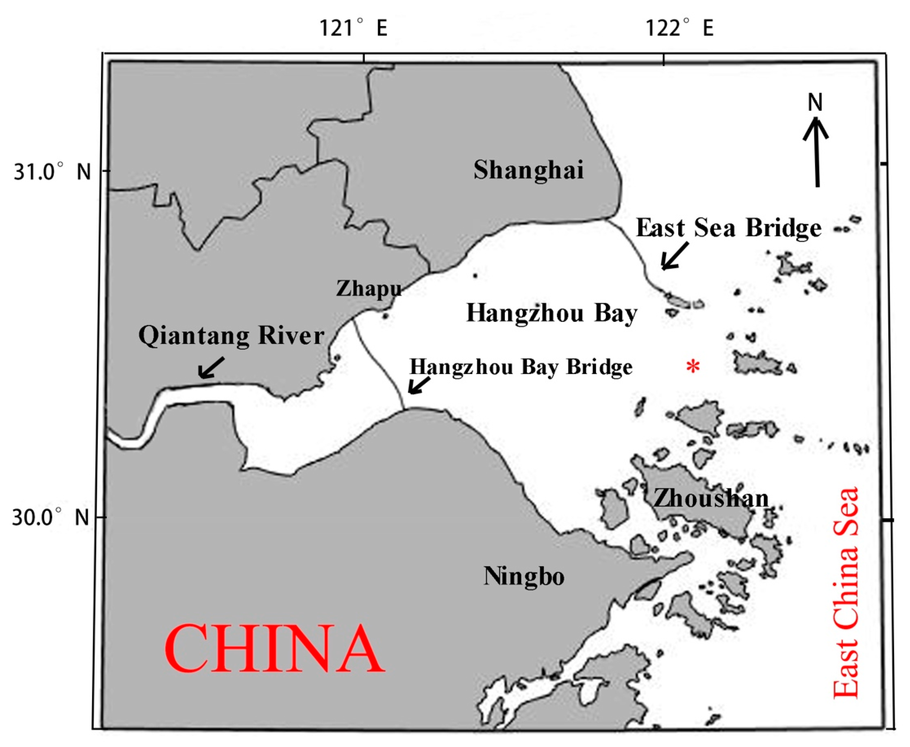
2.1. Study Area
2.2. Remote-Sensing Data
2.2.1. Landsat 8 Data
2.2.2. HY-1C Data
2.3. In Situ Data
2.4. Data Processing
2.4.1. Normalized Difference Vegetation Index (NDVI) Calculation
2.4.2. Vegetation Proportion Calculation
2.4.3. Land Surface Emissivity Estimation
2.4.4. An Improved Mono-Window Algorithm
2.4.5. SSC Retrieval
3. Result
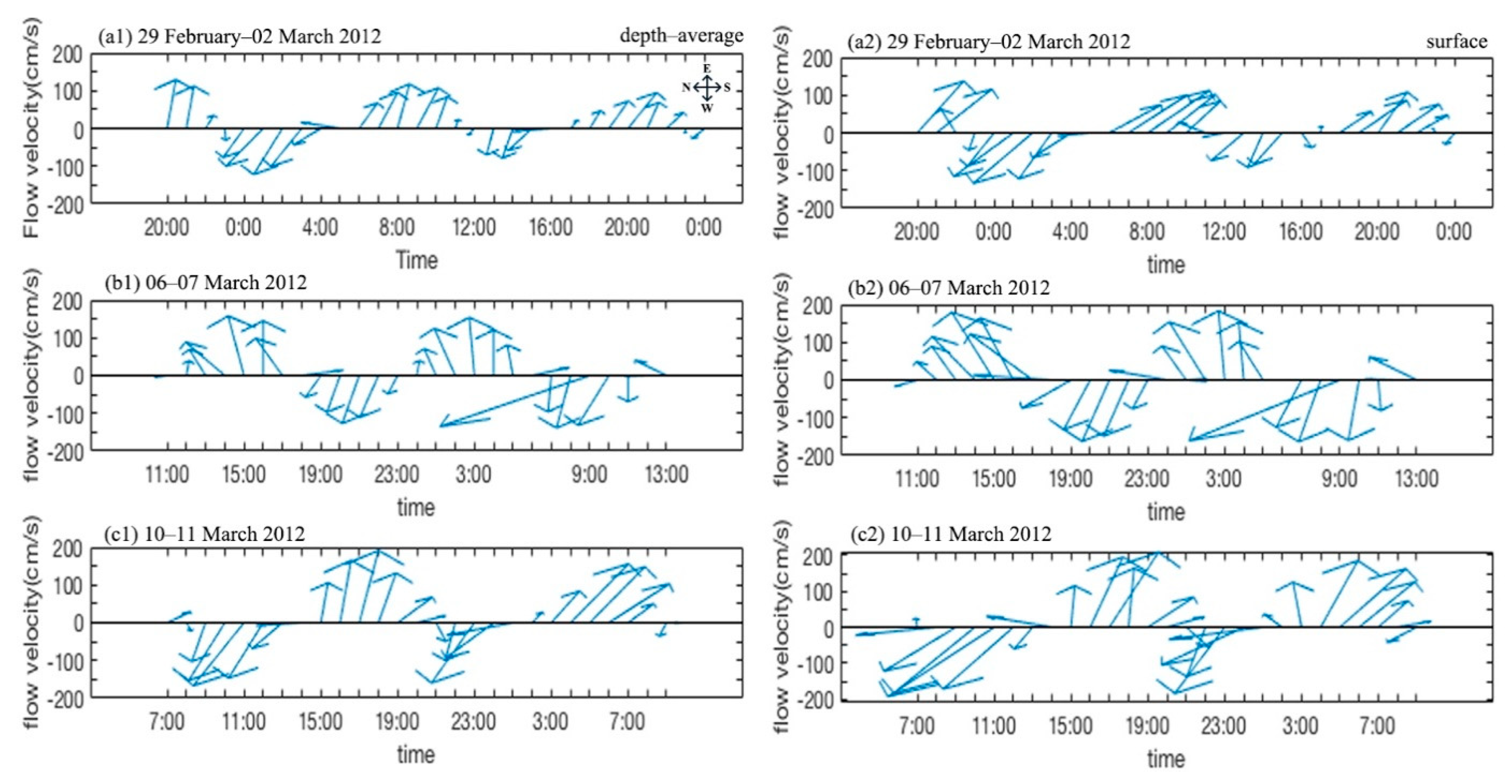
3.1. Tidal Current
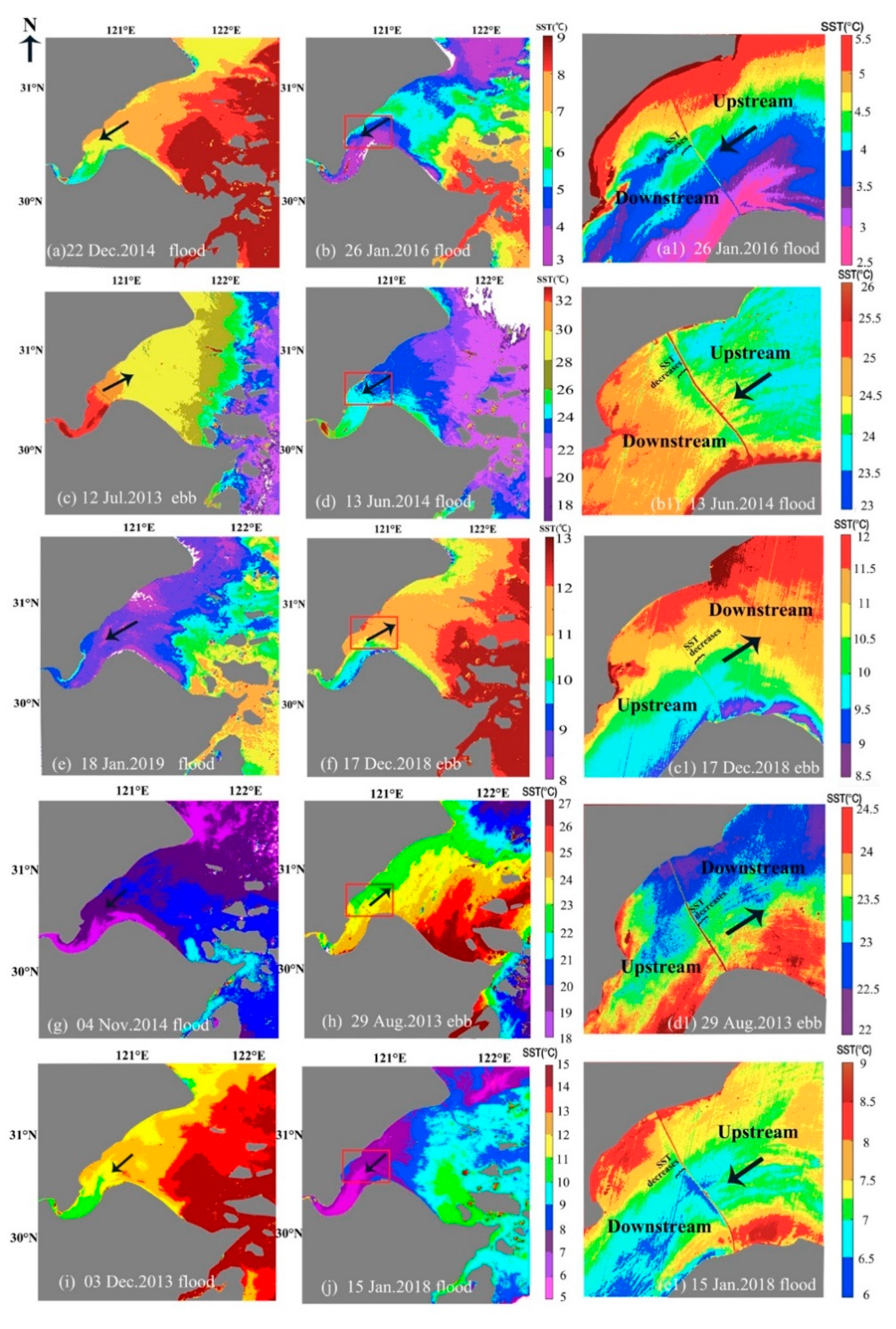
3.2. SST of Hangzhou Bay
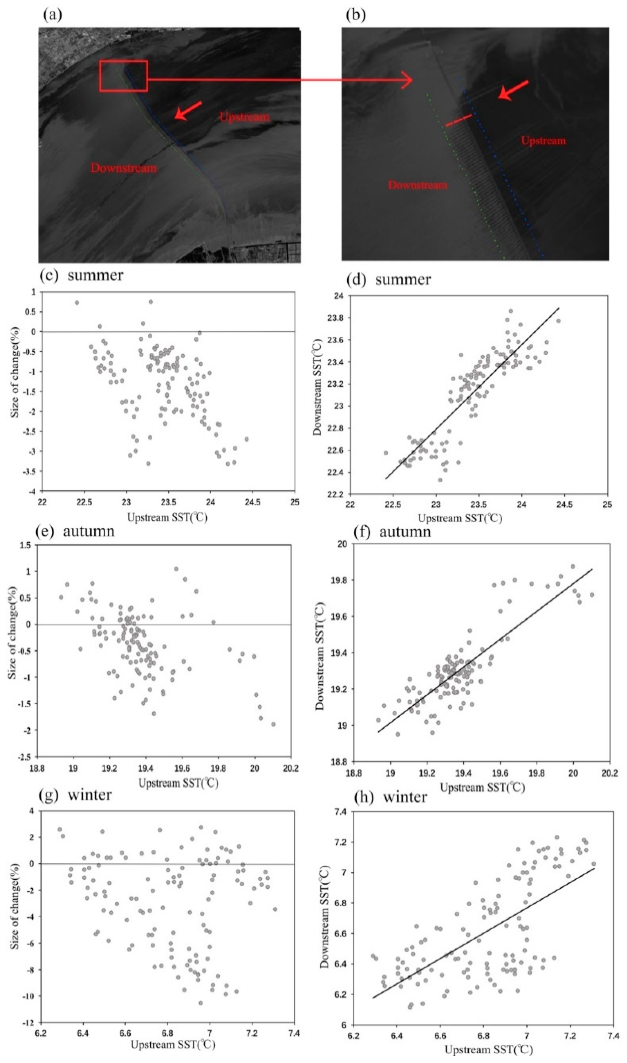
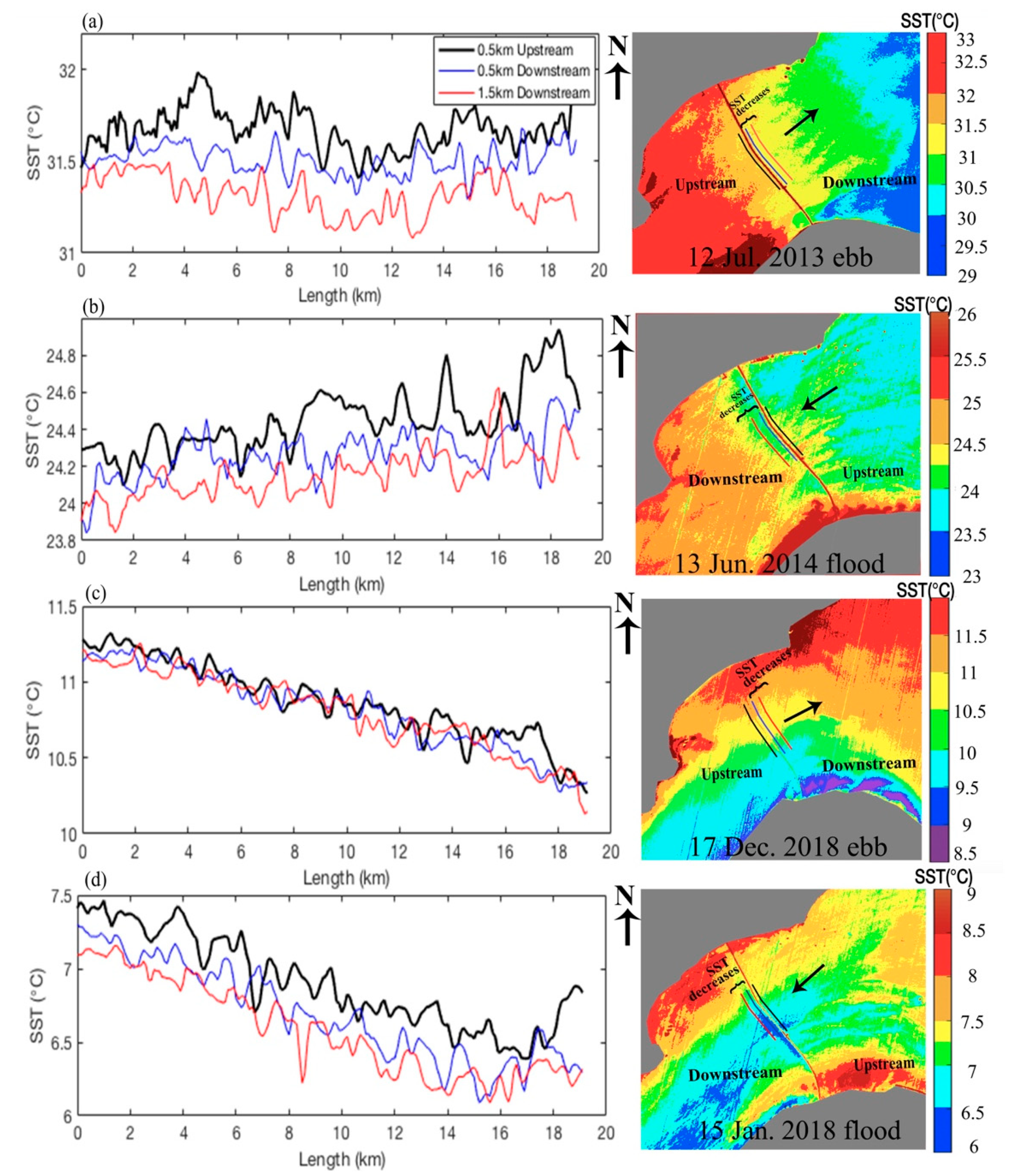
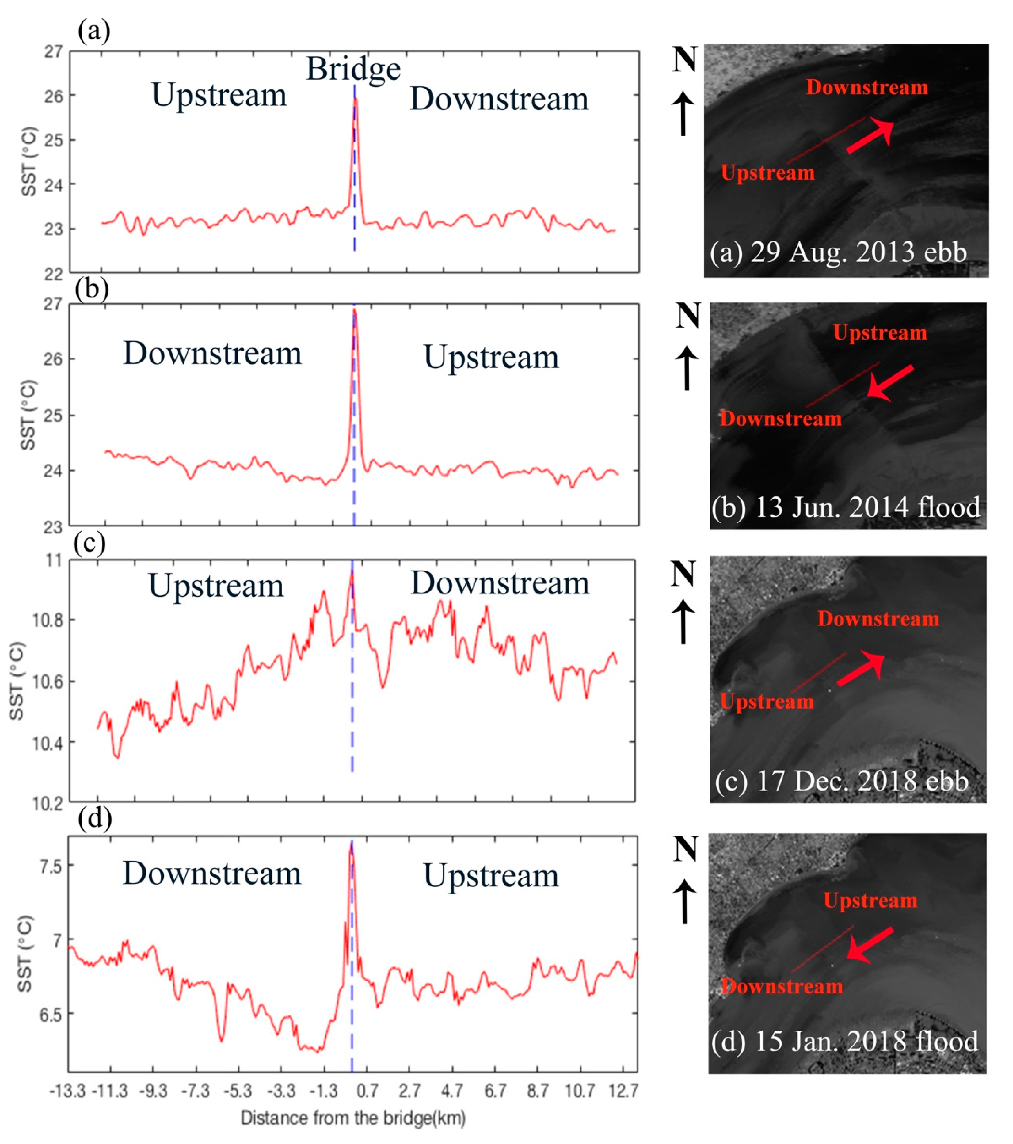
3.3. Decreased SST Downstream of the Bridges
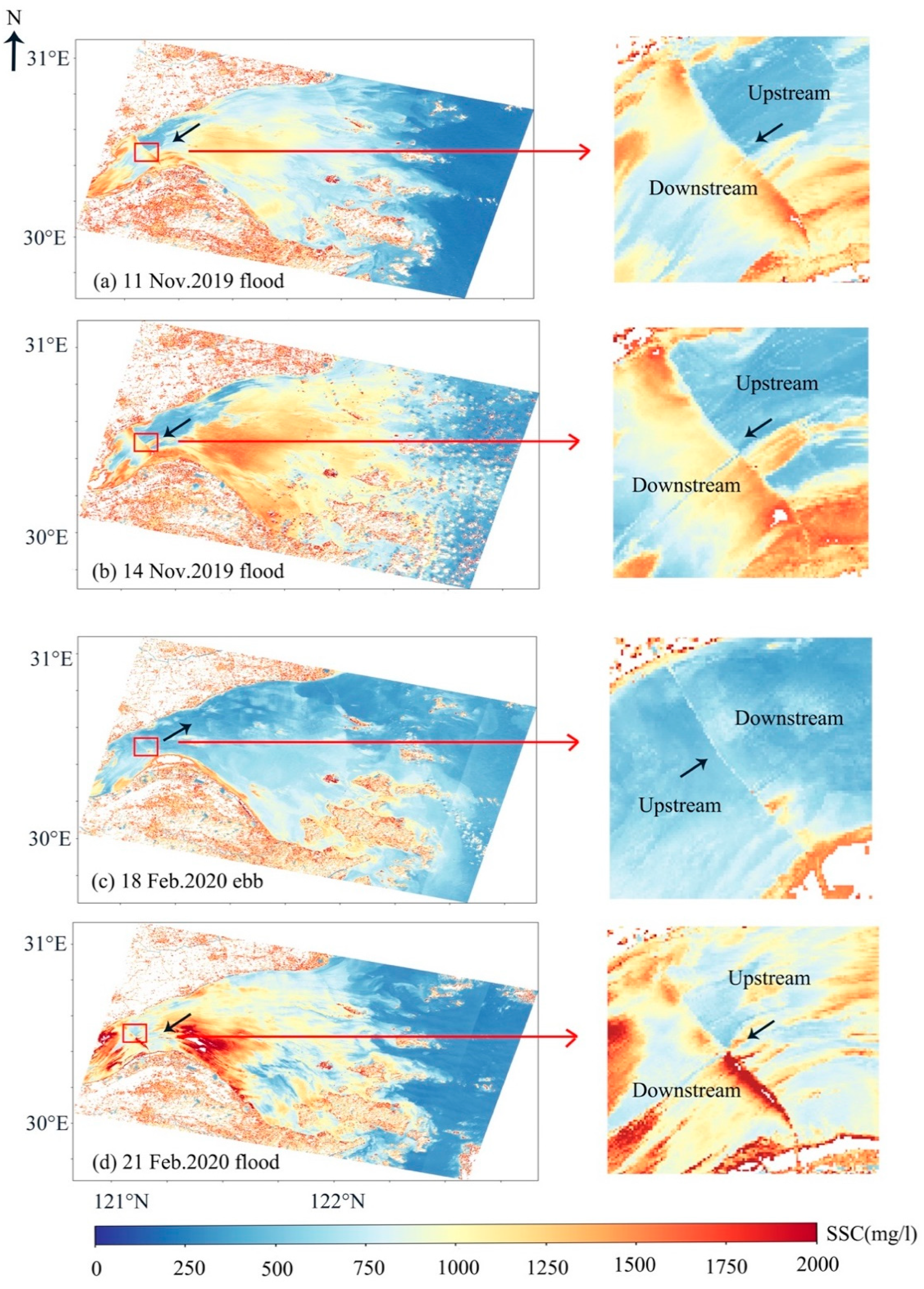
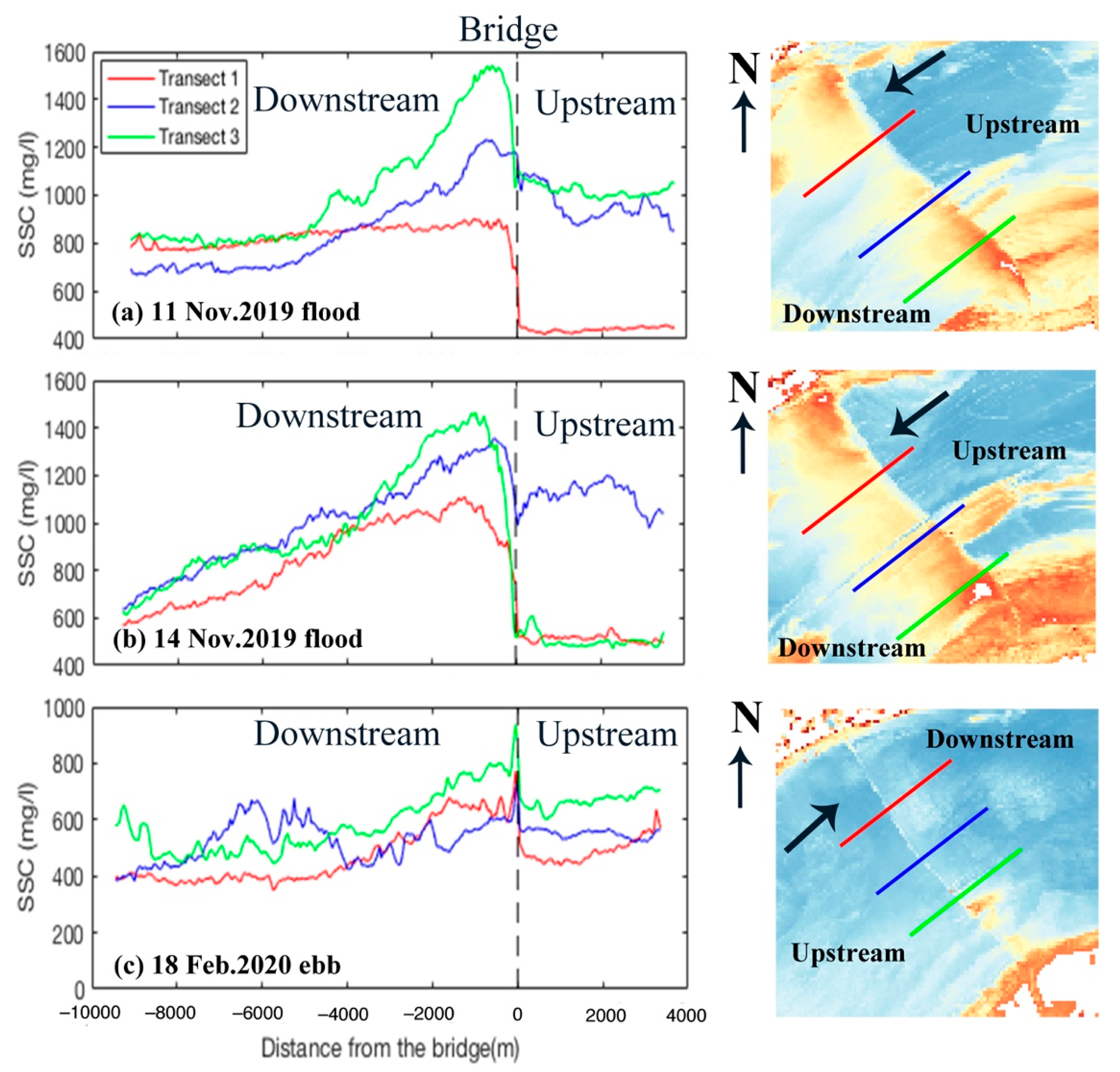
3.4. Increased SSC Downstream of the Bridges
4. Discussion
4.1. Factors Affecting SST Distribution in Hangzhou Bay
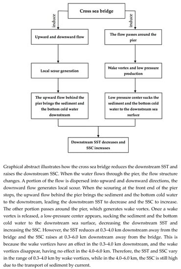
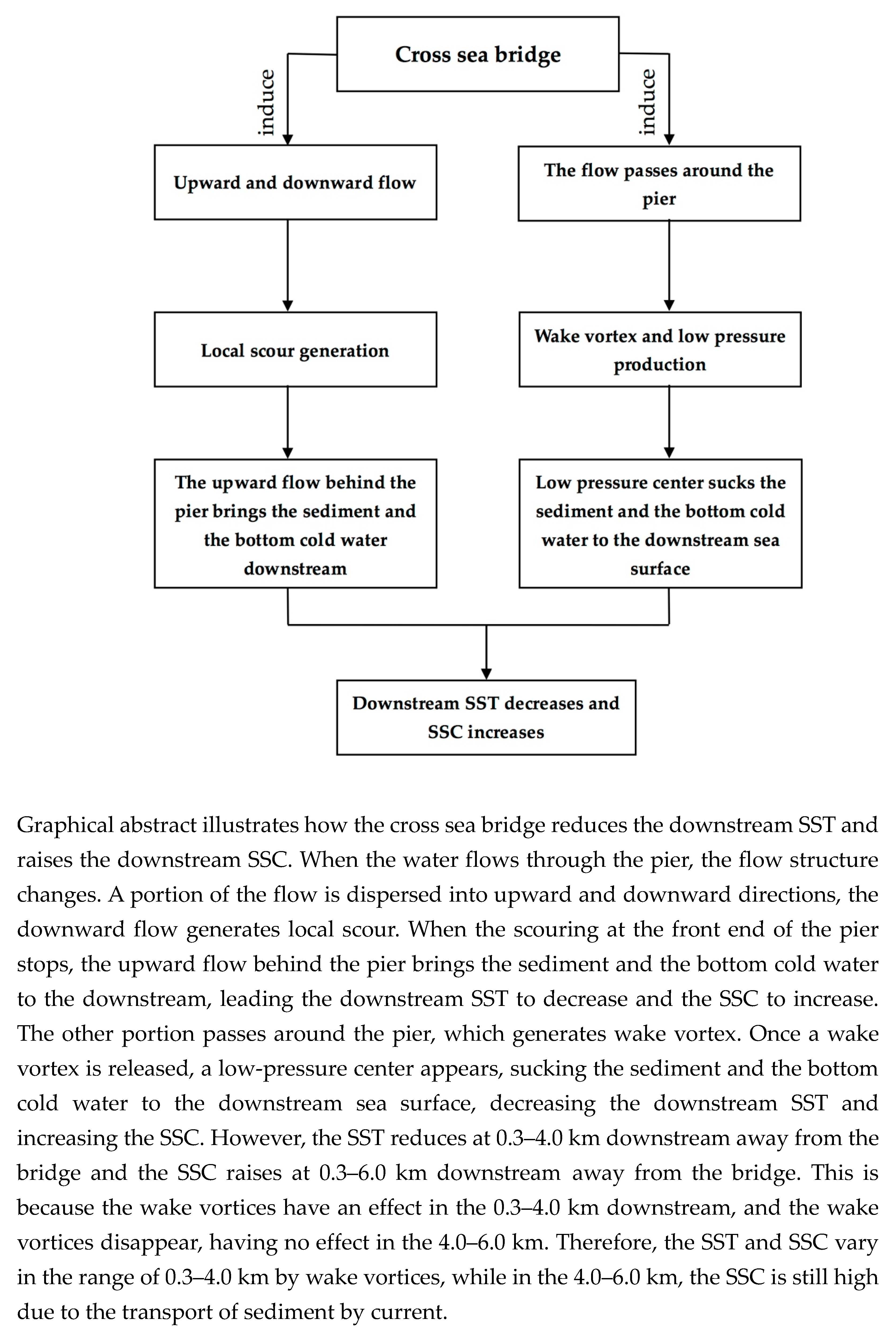
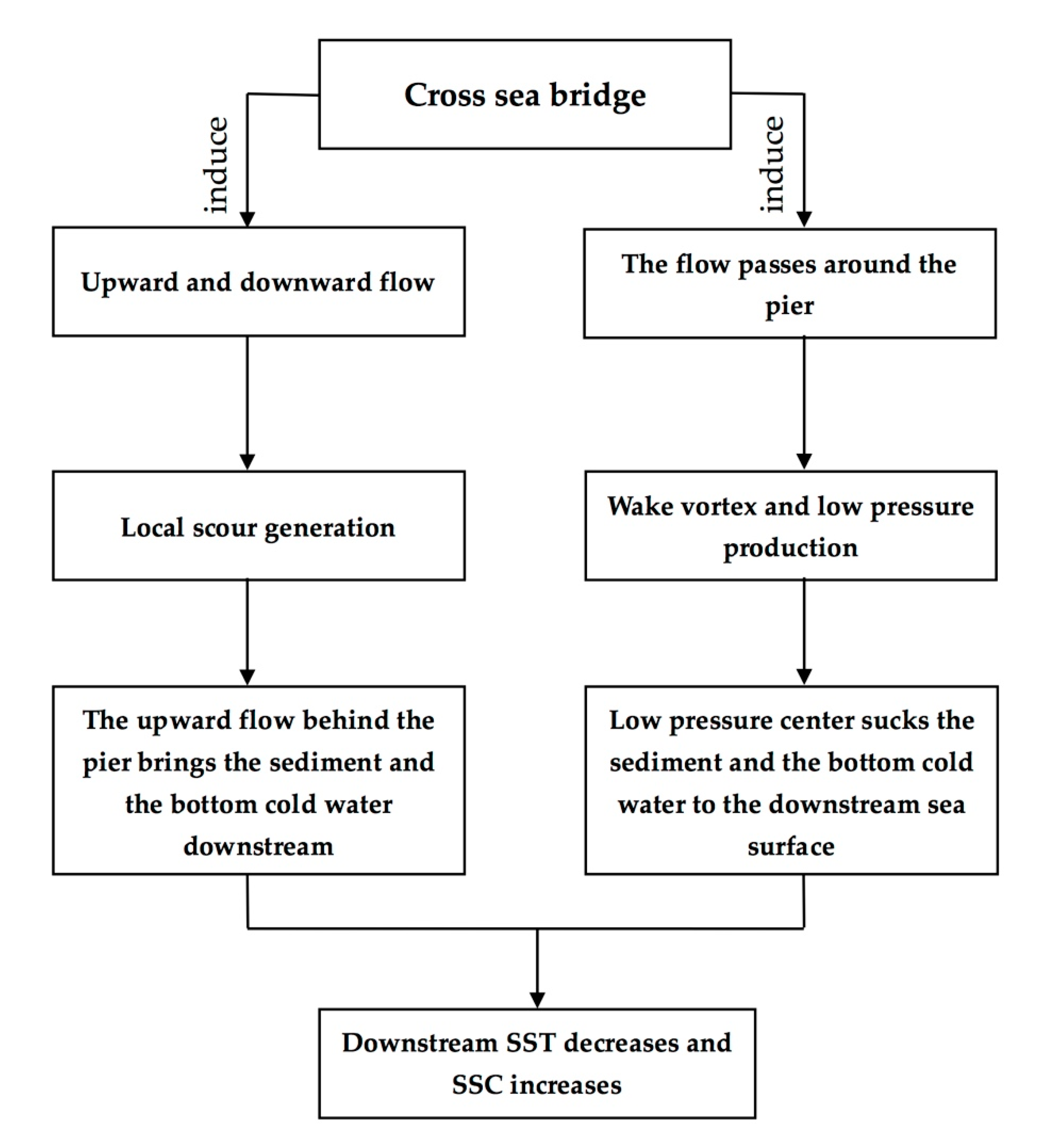
4.2. Influence of Cross-Sea Bridge on SST and SSC Distribution
4.3. Comparison of the Influence of the Pier on the SST and SSC
5. Conclusions
Author Contributions
Funding
Acknowledgments
Conflicts of Interest
References
- Li, P.; Li, G.; Qiao, L.; Chen, X.; Shi, J.; Gao, F.; Wang, N.; Yue, S. Modeling the tidal dynamic changes induced by the bridge in Jiaozhou Bay, Qingdao, China. Cont. Shelf Res. 2014, 84, 43–53. [Google Scholar] [CrossRef]
- Zhao, K.; Qiao, L.; Shi, J.; He, S.; Li, G.; Yin, P. Evolution of sedimentary dynamic environment in the western Jiaozhou Bay, Qingdao, China in the last 30 years. Estuar. Coast. Shelf Sci. 2015, 163, 244–253. [Google Scholar] [CrossRef]
- Qi, J. Mordern sedimentation rate and heavy metal accumulation in Jiaozhou Bay sediments. Science 2005, 308, 1293–1295. [Google Scholar]
- Qiao, S.; Pan, D.; He, X.; Cui, Q. Numerical Study of the Influence of Donghai Bridge on Sediment Transport in the Mouth of Hangzhou Bay. Procedia Environ. Sci. 2011, 10, 408–413. [Google Scholar] [CrossRef]
- Rasmusson, E.M.; Carpenter, T.H. Variations in tropical sea surface temperature and surface wind fields associated with the Southern Oscillation/El Niño. Mon. Wea. Rev. 1982, 110, 354–384. [Google Scholar] [CrossRef]
- Oka, E.; Kawabe, M. Characteristics of variations of water properties and density structure around the Kuroshio in the East China Sea. J. Oceanogr. 1998, 54, 605–617. [Google Scholar] [CrossRef]
- Sun, Y.; Sun, C.; Wang, X.; Tian, H.; Chen, S. Forecast of Impact of Qingdao Bay Bridge on Tide, Tidal Current and Residual Current of Jiaozhou Bay: I. Tidal Current of Jiaozhou Bay and Adjacent Sea Area; Ocean University Qingdao: Qingdao, China, 1994; pp. 105–119. [Google Scholar]
- Sun, Y.; Tian, H.; Zheng, L.; Chen, S. Forecast of Impact of Qingdao BayBridge on Tide, Tidal Current and Residual Current of Jiaozhou Bay: II. Study of Forecast Method; Ocean University Qingdao: Qingdao, China, 1994; pp. 120–125. [Google Scholar]
- Sun, Y.; Wang, X.; Sun, C.; Chen, S. Forecast of Impact of Qingdao Bay Bridge on Tide, Tidal Current and Residual Current of Jiaozhou Bay: III. Forecast Method and Forecast Results; Ocean University Qingdao: Qingdao, China, 1994; pp. 126–133. [Google Scholar]
- Cai, L.; Tang, D.; Levy, G.; Liu, D. Remote sensing of the impacts of construction in coastal waters on suspended particulate matter concentration—The case of the Yangtze River delta, China. Int. J. Remote Sens. 2016, 37, 2132–2147. [Google Scholar] [CrossRef]
- Cai, L.; Zhou, M.; Liu, J.; Tang, D.; Zuo, J. HY-1C Observations of the Impacts of Islands on Suspended Sediment Distribution in Zhoushan Coastal Waters, China. Remote. Sens. 2020, 12, 1766. [Google Scholar] [CrossRef]
- Li, J.; Gao, S.; Wang, Y.P. Delineating suspended sediment concentration patterns in surface waters of the Changjiang Estuary by remote sensing analysis. Acta Oceanol. Sin. 2010, 29, 38–47. [Google Scholar] [CrossRef]
- Hu, Y.; Yu, Z.; Zhou, B.; Li, Y.; Yin, S.; He, X.; Peng, X.; Shum, C. Tidal-driven variation of suspended sediment in Hangzhou Bay based on GOCI data. Int. J. Appl. Earth Obs. Geoinf. 2019, 82. [Google Scholar] [CrossRef]
- Tanimoto, Y.; Nakamura, H.; Kagimoto, T.; Yamane, S. An active role of extratropical sea surface temperature anomalies in determining anomalous turbulent heat flux. J. Geophys. Res. Space Phys. 2003, 108, 108. [Google Scholar] [CrossRef]
- Yeh, S.; Kim, C.-H. Recent warming in the Yellow/East China Sea during winter and the associated atmospheric circulation. Cont. Shelf Res. 2010, 30, 1428–1434. [Google Scholar] [CrossRef]
- Deng, Z.; Xie, L.; Han, G.; Zhang, X.; Wu, K. The effect of Coriolis-Stokes forcing on upper ocean circulation in a two-way coupled wave-current model. Chin. J. Oceanol. Limnol. 2012, 30, 321–335. [Google Scholar] [CrossRef]
- Jiménez-Muñoz, J.C.; Sobrino, J.A. A generalized single-channel method for retrieving land surface temperature from remote sensing data. J. Geophys. Res. 2003, 108. [Google Scholar] [CrossRef]
- Qin, Z.; Karnieli, A.; Berliner, P. A mono-window algorithm for retrieving land surface temperature from Landsat TM data and its application to the Israel-Egypt border region. Int. J. Remote Sens. 2001, 22, 3719–3746. [Google Scholar] [CrossRef]
- Wang, F.; Qin, Z.; Song, C.; Tu, L.; Karnieli, A.; Zhao, S. An Improved Mono-Window Algorithm for Land Surface Temperature Retrieval from Landsat 8 Thermal Infrared Sensor Data. Remote Sens. 2015, 7, 4268–4289. [Google Scholar] [CrossRef]
- McConaghy, D.C. Measuring sea surface temperature from satellites: A ground truth approach. Remote Sens. Environ. 1980, 10, 307–310. [Google Scholar] [CrossRef]
- Saldías, G.S.; Lara, C. Satellite-derived sea surface temperature fronts in a river-influenced coastal upwelling area off central-southern Chile. Reg. Stud. Mar. Sci. 2020, 37, 101322. [Google Scholar] [CrossRef]
- Unger, J.; Hager, W.H. Down-flow and horseshoe vortex characteristics of sediment embedded bridge piers. Exp. Fluids 2007, 42, 1–19. [Google Scholar] [CrossRef]
- Zhou, Y.; Wang, Y. Forecast of the Bridge Local Scour Depth. J. Xi’an Highw. Univ. 1999, 19, 48–50. [Google Scholar]
- Wang, F.; Zhou, B.; Xu, J.; Song, L.; Wang, X. Application of neural network and MODIS 250 m imagery for estimating suspended sediments concentration in Hangzhou Bay, China. Environ. Geol. 2009, 56, 1093–1101. [Google Scholar] [CrossRef]
- Liu, C.; Sui, J.; He, Y.; Hirshfield, F. Changes in runoff and sediment load from major Chinese rivers to the Pacific Ocean over the period 1955–2010. Int. J. Sediment Res. 2013, 28, 486–495. [Google Scholar] [CrossRef]
- Xie, D.; Wang, Z.B.; Gao, S.; De Vriend, H. Modeling the tidal channel morphodynamics in a macro-tidal embayment, Hangzhou Bay, China. Cont. Shelf Res. 2009, 29, 1757–1767. [Google Scholar] [CrossRef]
- Xie, D.; Gao, S.; Wang, Z.B.; Pan, C.-H. Numerical modeling of tidal currents, sediment transport and morphological evolution in Hangzhou Bay, China. Int. J. Sediment Res. 2013, 28, 316–328. [Google Scholar] [CrossRef]
- Ni, Y.Q.; Geng, Z.Q.; Zhu, J.Z. Study on characteristic of hydrodynamics in Hangzhou Bay. J. Hydrodyn. 2003, 18, 439–445. [Google Scholar]
- Zhang, Z.; Wu, C.; Huo, Y. The principle of a model SLC9-2 current meter and its handling. J. Mar. Sci. 2000, 1, 61–64. [Google Scholar]
- Wang, S.M.; Wang, Z.; He, Q.Y.; Zhang, J.; Zhang, Y.Q. Structure Design of the ANSYS-Based SLC9-2-Type Direct Reading Current Meter. Adv. Mater. Res. 2014, 926, 1412–1416. [Google Scholar] [CrossRef]
- Zhu, W.; Pang, S.; Chen, J.; Sun, N.; Huang, L.; Zhang, Y.; Zhang, Z.; He, S.; Cheng, Q. Spatiotemporal variations of total suspended matter in complex archipelagic regions using a sigmoid model and Landsat-8 imagery. Reg. Stud. Mar. Sci. 2020, 36, 101308. [Google Scholar] [CrossRef]
- Carlson, T.N.; Ripley, D.A. On the relation between NDVI, fractional vegetation cover, and leaf area index. Remote Sens. Environ. 1997, 62, 241–252. [Google Scholar] [CrossRef]
- Sobrino, J.A.; Raissouni, N. Toward remote sensing methods for land cover dynamic monitoring: Application to Morocco. Int. J. Remote Sens. 2000, 21, 353–366. [Google Scholar] [CrossRef]
- Sobrino, J.A.; Jiménez-Muñoz, J.C.; Paolini, L. Land surface temperature retrieval from LANDSAT TM 5. Remote Sens. Environ. 2004, 90, 434–440. [Google Scholar] [CrossRef]
- Sobrino, J.A.; Jimenez-Munoz, J.C.; Soria, G.; Romaguera, M.; Guanter, L.; Moreno, J.; Plaza, J.; Martinez, P.; Jimenez-Muoz, J. Land Surface Emissivity Retrieval from Different VNIR and TIR Sensors. IEEE Trans. Geosci. Remote. Sens. 2008, 46, 316–327. [Google Scholar] [CrossRef]
- Wen-Yao, L.; Field, R.; Gantt, R.; Klemas, V. Measurement of the surface emissivity of turbid waters. Remote Sens. Environ. 1987, 21, 97–109. [Google Scholar] [CrossRef]
- Wang, L.; Lu, Y.; Yao, Y. Comparison of Three Algorithms for the Retrieval of Land Surface Temperature from Landsat 8 Images. Sensors 2019, 19, 5049. [Google Scholar] [CrossRef]
- Nikam, B.R.; Ibragimov, F.; Chouksey, A.; Garg, V.; Aggarwal, S.P. Retrieval of land surface temperature from Landsat 8 TIRS for the command area of Mula irrigation project. Environ. Earth Sci. 2016, 75, 1169. [Google Scholar] [CrossRef]
- Hadjimitsis, D.G.; Hadjimitsis, M.G.; Clayton, C.R.I.; Clarke, B.A. Determination of Turbidity in Kourris Dam in Cyprus Utilizing Landsat TM Remotely Sensed Data. Water Resour. Manag. 2006, 20, 449–465. [Google Scholar] [CrossRef]
- Lenoble, J.; Herman, M. Radiative transfer in the Earth’s atmosphere. Aerosol Remote Sens. 2013, 53–86. [Google Scholar] [CrossRef]
- Chen, X.-Y.; Zhang, J.; Tong, C.; Liu, R.-J.; Mu, B.; Ding, J. Retrieval Algorithm of Chlorophyll-a Concentration in Turbid Waters from Satellite HY-1C Coastal Zone Imager Data. J. Coast. Res. 2019, 90, 146–155. [Google Scholar] [CrossRef]
- Cho, Y.-K.; Lee, K.-S.; Park, K.-Y. Year-to-year Variability of the Vertical Temperature Structure in the Youngsan Estuary. Ocean Polar Res. 2009, 31, 239–246. [Google Scholar] [CrossRef]
- Padilla, E.M.; Díez-Minguito, M.; Sánchez, M.O.; Losada, M.A. A Subtidal Model of Temperature for a Well-Mixed Narrow Estuary: The Guadalquivir River Estuary (SW Spain). Chesap. Sci. 2015, 39, 605–620. [Google Scholar] [CrossRef]
- Liu, X.-Q.; Yin, B.-S.; Hou, Y.-J. The dynamic of circulation and temperature-salinity structure in the changjiang mouth and its adjacent marine area II. Major characteristics of the circulation. Oceanol. Limnol. Sin. 2008, 39, 312–320. [Google Scholar]
- Zhou, X.-Y.; Hu, D.-B.; Wang, C.-Z.; Hu, X.-J.; Yao, S.-K. Seasonal and Interannual SST Variations in the Changjiang Estuary. J. Ocean Univ. Qingdao 2005, 35, 357–362. [Google Scholar]
- Li, S.; Sun, W. Numerical Modeling of Residual Currents in Hangzhou Bay. Oceanol. Limnol. Sin. 1995, 26, 254–261. [Google Scholar]
- Wang, Q.; Li, Z. Numerical simulation of water temperature under diurnal variation of air temperature in the Hangzhou Bay. Mar. Sci. Bull. 2018, 37, 303–309. [Google Scholar]
- Zhu, Q.; He, J.; Wang, P. A study of circulation differences between East-Asian and Indian summer monsoons with their interaction. Adv. Atmos. Sci. 1986, 3, 466–477. [Google Scholar]
- Zou, T.; Gao, H.-W.; Sun, W.-X.; Liu, Z. Numerical Simulation of Lagrange Residual Current in the Changjiang Estuary, Hangzhou Bay and Their Adjacent Sea I: Barotropic Circulation. Period. Ocean Univ. China 2009, 39, 153–159. [Google Scholar]
- Liu, X.-Q.; Hou, Y.-J.; Yin, B.-S.; Yang, D.-Z. Dynamics of circulation and temperature-salinity structures in changjiang river mouth and its adjacent sea III. The temperature structure. Oceanol. Limnol. Sin. 2015, 46, 526–533. [Google Scholar]
- Liu, X.; Lu, Y.; Pan, L. Tidal current numerical simulating and water exchange research in Yangtze Estuary and Hangzhou Bay. J. Hydrodyn. 2006, 21, 171–180. [Google Scholar]
- Zhang, F.; Wu, T. Sediment concentration measurement based on thermal capacity. J. Hohai Univ. (Nat. Sci.) 2013, 41, 456–460. [Google Scholar]
- Pan, C.; Huang, W. Numerical Modeling of Suspended Sediment Transport Affected by Tidal Bore in Qiantang Estuary. J. Coast. Res. 2010, 26, 1123–1132. [Google Scholar] [CrossRef]
- Li, L.; Taoyan, Y.; Lu, Z.; Yanming, Y.; Yuezhang, X. Influences of reclamation location on the water and sediment environment in Hangzhou Bay. J. Harbin Eng. Univ. 2019, 40, 1870–1875. [Google Scholar]
- Chen, X. The Analysis of Multitemporal Remote Sensing Images for Suspended Sediment in Hangzhou Bay. J. Remote Sens. 1989, 128–135. [Google Scholar]
- Zhang, X.-Y.; Lv, H.-X.; Shen, B. Experimental studies on local scour mechanism of cylinder bridge piers. Hydro Sci. Eng. 2012, 2, 34–41. [Google Scholar]
- Qi, M.-L. Riverbed scouring around bridge piers in river section with sand pits. J. Hydraul. Eng. 2005, 7, 835–839. [Google Scholar]
- Olsen, N.R.B.; Kjellesvig, H.M. Three-dimensional numerical flow modeling for estimation of maximum local scour depth. J. Hydraul. Res. 1998, 36, 579–590. [Google Scholar] [CrossRef]
- Pasiok, R.; Stilger-Szydło, E. Sediment particles and turbulent flow simulation around bridge piers. Arch. Civ. Mech. Eng. 2010, 10, 67–79. [Google Scholar] [CrossRef]
- Roulund, A.; Sumer, B.M.; Fredsøe, J.; Michelsen, J. Numerical and experimental investigation of flow and scour around a circular pile. J. Fluid Mech. 2005, 534, 351–401. [Google Scholar] [CrossRef]
- Su, J.; Wang, K.; Li, Y. Fronts and transport of suspended matter in the Hangzhou Bay. Acta Oceanol. Sin. 1993, 12, 1–15. [Google Scholar]


| Sensor | Band | Spatial Resolution (m) | |
|---|---|---|---|
| OLI | Band1-COASTAL | 0.433–0.453 | 30 |
| Band2-Blue | 0.450–0.515 | 30 | |
| Band3-Green | 0.525–0.600 | 30 | |
| Band4-Red | 0.630–0.680 | 30 | |
| Band5-NIR | 0.845–0.885 | 30 | |
| Band6-SWIR1 | 1.560–1.660 | 30 | |
| Band7-SWIR2 | 2.100–2.300 | 30 | |
| Band8-PAN | 0.500–0.680 | 15 | |
| Band9-Cirrus | 1.360–1.390 | 30 | |
| TIRS | Band10-TIR | 10.60–11.19 | 100 |
| Band11-TIR | 11.50–12.51 | 100 |
| Number | Band | Acquired Date |
|---|---|---|
| 1 | Band10-TIR | 12 July 2013 |
| 2 | Band10-TIR | 29 August 2013 |
| 3 | Band10-TIR | 3 December 2013 |
| 4 | Band10-TIR | 13 June 2014 |
| 5 | Band10-TIR | 4 November 2014 |
| 6 | Band10-TIR | 22 December 2014 |
| 7 | Band10-TIR | 26 January 2016 |
| 8 | Band10-TIR | 15 January 2018 |
| 9 | Band10-TIR | 17 December 2018 |
| 10 | Band10-TIR | 18 January 2019 |
| Band | Spatial Resolution (m) | Date | |
|---|---|---|---|
| Band1-Blue | 0.421–0.500 | 50 | 11 November 2019 |
| Band2-Green | 0.517–0.598 | 50 | 14 November 2019 |
| Band3-Red | 0.608–0.690 | 50 | 18 February 2020 |
| Band4-NIR | 0.761–0.891 | 50 | 21 February 2020 |
| Number | Location | Time | Measurements Taken |
|---|---|---|---|
| 1 | 30.35° N, 122.13° E | 29 February–2 March 2012 | Depth |
| 2 | 30.35° N, 122.13° E | 6–7 March 2012 | Velocity and direction of flow |
| 3 | 30.35° N, 122.13° E | 10–11 March 2012 |
© 2020 by the authors. Licensee MDPI, Basel, Switzerland. This article is an open access article distributed under the terms and conditions of the Creative Commons Attribution (CC BY) license (http://creativecommons.org/licenses/by/4.0/).
Share and Cite
Huang, S.; Liu, J.; Cai, L.; Zhou, M.; Bu, J.; Xu, J. Satellites HY-1C and Landsat 8 Combined to Observe the Influence of Bridge on Sea Surface Temperature and Suspended Sediment Concentration in Hangzhou Bay, China. Water 2020, 12, 2595. https://doi.org/10.3390/w12092595
Huang S, Liu J, Cai L, Zhou M, Bu J, Xu J. Satellites HY-1C and Landsat 8 Combined to Observe the Influence of Bridge on Sea Surface Temperature and Suspended Sediment Concentration in Hangzhou Bay, China. Water. 2020; 12(9):2595. https://doi.org/10.3390/w12092595
Chicago/Turabian StyleHuang, Shuyi, Jianqiang Liu, Lina Cai, Minrui Zhou, Juan Bu, and Jieni Xu. 2020. "Satellites HY-1C and Landsat 8 Combined to Observe the Influence of Bridge on Sea Surface Temperature and Suspended Sediment Concentration in Hangzhou Bay, China" Water 12, no. 9: 2595. https://doi.org/10.3390/w12092595
APA StyleHuang, S., Liu, J., Cai, L., Zhou, M., Bu, J., & Xu, J. (2020). Satellites HY-1C and Landsat 8 Combined to Observe the Influence of Bridge on Sea Surface Temperature and Suspended Sediment Concentration in Hangzhou Bay, China. Water, 12(9), 2595. https://doi.org/10.3390/w12092595