Assessing Climate Change Effects on Water Balance in a Monsoon Watershed

Abstract

Understanding the changes on future water resources resulting from climate variations will assist in developing effective management strategies for a river basin. Our area of interest is the Osan watershed in South Korea, where the summer monsoon contributes approximately 60–70% of the annual runoff and precipitation for the country. We determined the effects that future climatic changes have on this area. To accomplish this, we made use of global climate models (GCMs). A total of 10 GCMs were downscaled with the help of climate information production tools. Coupled with the GCMs and the Soil and Water Assessment (SWAT) model, three periods were used to assess these climate impacts. The baseline, mid-century (MC), and end-century (EC) periods include 1993–2018, 2046–2065, and 2081–2099, respectively. The entire process was performed using two scenarios (4.5 and 8.5) from the representative concentration pathways (RCPs). Some of the statistical metrics used for model calibration and validation were p-factor, r-factor, percent bias, root-mean-square error (RMSE), and Nash–Sutcliffe model efficiency. Their respective values were 0.88, 0.88, 8.3, 0.91, and 0.91 for calibration, and 1.16, 0.85, 7.9, 0.88, and 0.87 for validation. For the MC and EC periods under both scenarios, we projected an increase in temperature and precipitation of approximately 2–5 °C and 15–30%, respectively. A predicted rise in precipitation, surface flow, lateral flow, and water yield were noted for the month of June. Subsequently, a decline in July followed during the summer monsoon season. Summer monsoon rains will fluctuate more sharply, with heavy rainfall in June, lower rainfall in July, and more rain in the late summer, leading to the possibility of both flooding and drought within a given period. Annual precipitation, surface flow, lateral flow, and water yield will increase whereas evapotranspiration would decrease in both periods under both scenarios during the summer monsoon period, which will lead to wetter conditions in the future.

1. Introduction

Recurring changes in the climate have been predicted to detrimentally affect water resources on a global scale [1]. The water balance in river basins is known to be widely affected by human activities, and abrupt environmental and climatic changes [2]. In an attempt to document the effect of these changes, environmental organizations have developed climate models to project the consequences of future climate change based on representative concentration pathways (RCPs) for greenhouse gases extending to 2100. An example of such an organization is the World Climate Research Programme (WCRP), which has developed numerous climate models at a global scale (GCMs) under their Coupled Model Intercomparison Project 5 (CMIP5) program [3]. Using these GCMs to determine future changes in the water balance will aid in putting forward adaptation and management strategies to tackle the adverse effects of our changing climate on available water resources.

According to National Institute for Meteorological Research in South Korea, east Asia is expected to experience a temperature rise of 3–4 °C by 2100 [4]. Evapotranspiration (ET) is generally predicted to increase with the rise in temperature, leading to an increase in air humidity and thus affecting rainfall [5]. For example, in South Korea, annual precipitation has increased from 754 mm in 1939 to 1756 mm in 2003, with a greater frequency of extreme flooding and drought events [6]. About 68% of the total precipitation occurs between June and September, thus any significant change in precipitation patterns could mean that the region is more prone to drought and/or flooding [7].

Hydrological models and GCMs are essential in evaluating the effects on future water balance changes. The Soil and Water Assessment Tool (SWAT) model (Texas A&M university, College Station, TX, USA) [8,9] in conjunction with GCMs [9,10] has been utilized in determining climate change effects on river basins. Due to its wide accessibility and user-friendly managing of data input, the SWAT has been widely used in hydrological modeling [11,12] and research on the impact of climate change [10,13,14]. Yan et al. [15] evaluated future changes in Miyun Reservoir basin, China on water quality streamflow. It was found that the watershed would become more humid and warmer by mid-century, thus the average annual precipitation, streamflow, and total nitrogen loading were expected to rise, especially during the summer. The impact of climate change on the Himalayan river basin was assessed by Bhatta et al. [14], who reported that the temperature would rise, and precipitation would decrease by 2100, leading to lower streamflow and a negative impact on the Tamor River basin. Ercan et al. [10] estimated the potential effects on the water balance in the Upper Neuse watershed, USA. They suggested that the water yield, precipitation, and soil water would increase whereas ET would decrease, with wetter conditions in the future.

In South Korea, the SWAT model has been used as a tool for water management [16], drought assessment [17], water quality assessment [18], hydrologic partitioning [19], water balance analysis [20], and prediction of the effects of changes on future water resources [21,22,23,24,25,26]. Future changes on hydrological parameters were evaluated by Joh et al. [27] for a heterogeneous forest drainage basin. Their results showed that temperature, precipitation, and ET would increase, whereas streamflow and soil moisture would decrease by mid and late century. Similarly, Nkomozepi and Chung [28] modeled the hydrology in the Geumo watershed in South Korea using five GCMs under RCPs 2.6, 4.5, and 8.5. Temperature and rainfall were expected to increase, and runoff and the aridity index would decrease in the future. In addition, future climate changes on groundwater levels for the Geum River, South Korea, were evaluated by Lee et al. [21], with the groundwater level predicted to fall both up- and downstream of some of the monitored points.

Many of the previous studies have demonstrated significant uncertainty in their climate projections due to variability between models [29]. In this respect, GCMs from CMIP5 offer improvements in physical parameterization and lateral resolution over previous models [30,31,32,33]. In addition, previous studies of climate change in South Korea have generally been based on a single water balance component (either surface flow, ET, or groundwater recharge) and a single GCM, while others have focused only on precipitation and temperature in terms of hydrology. Only a few studies have investigated more than one water balance component with multiple GCMs. In particular, in our study area, no prior research was carried out on the future climate change effects on multiple water balance components using multiple GCMs. Furthermore, Osan stream is used in irrigating paddy rice farming, which depends on precipitation during the summer monsoon season. Filling this gap will aid in understanding water resource trends for various climate change scenarios. Multiple climate scenarios have become the common procedure for characterizing uncertainty in the future climate [34].

In summary, we seek to understand the hydrological impacts on the Osan stream watershed for various climate change scenarios. Coupled with GCMs and the SWAT model, three periods were used to assess these climate impacts. The baseline, mid-century (MC), and end-century (EC) periods included 1993–2018, 2046–2065, and 2081–2099, respectively. Sensitivity and uncertainty analysis was done. Six statistical metrics were used for model calibration and validation. The impacts on future water balance were investigated using 10 downscaled GCMs in the MC and EC periods in the Osan watershed under the RCP 4.5 and 8.5.

2. Data Collection and Methodology

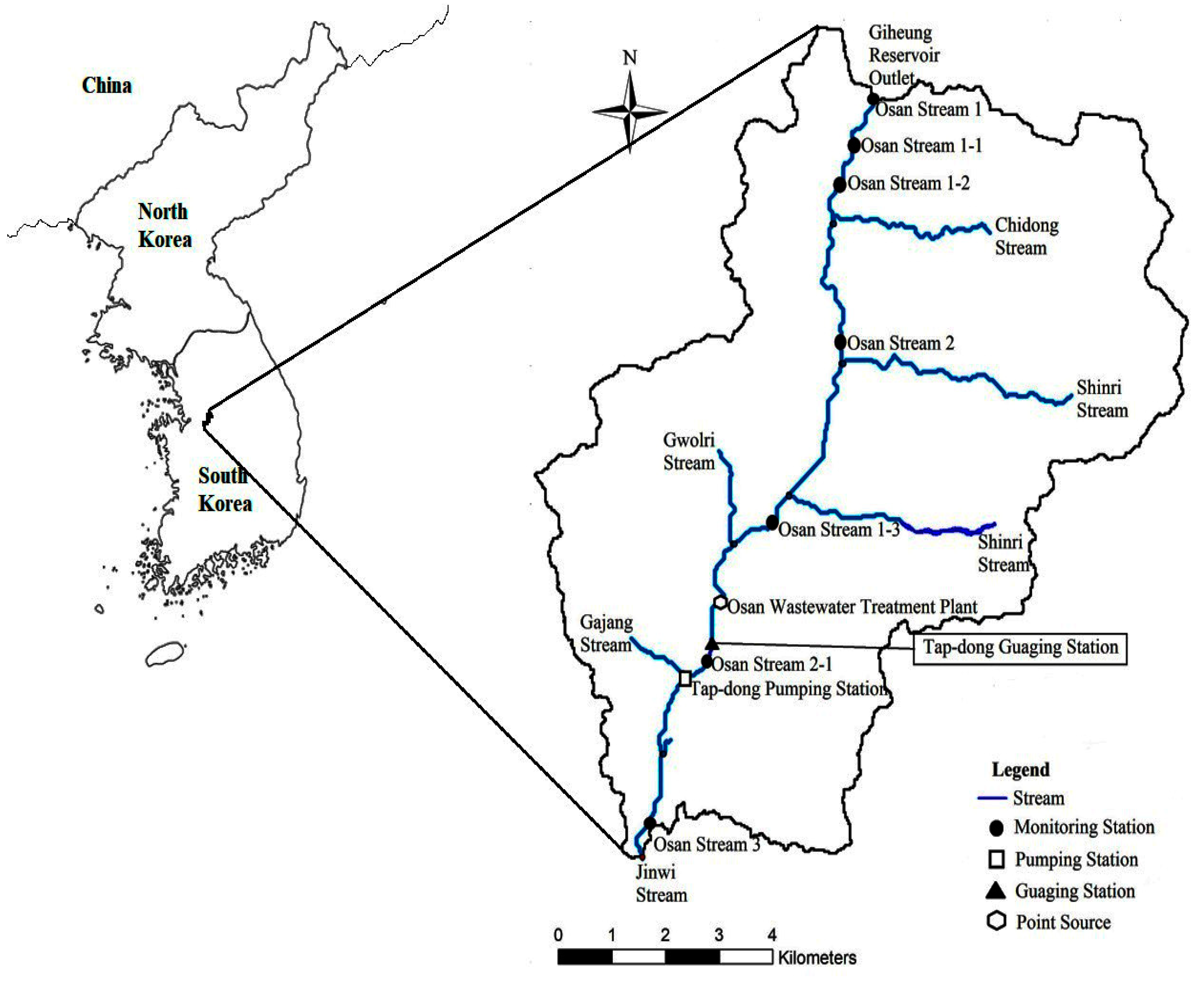
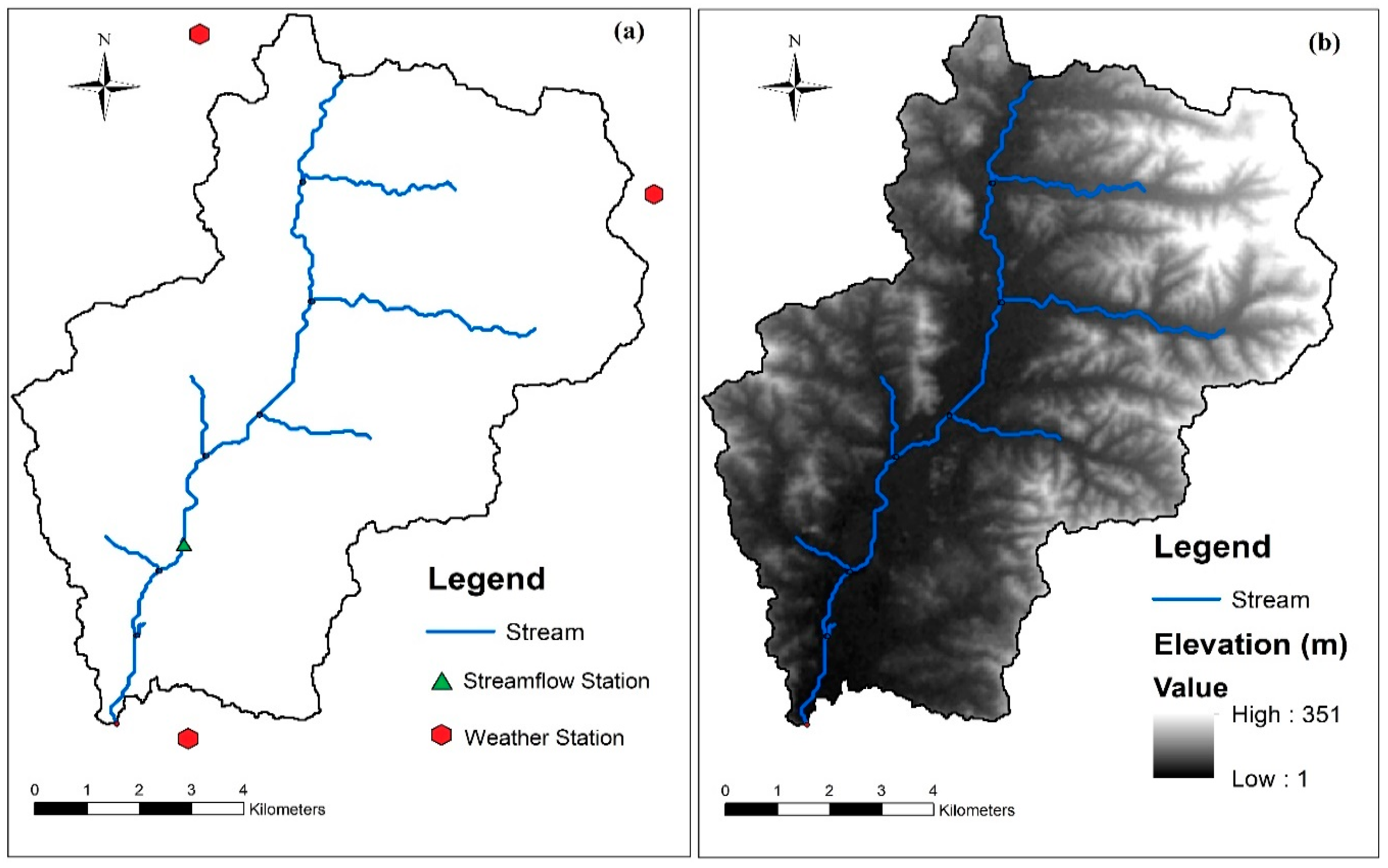
2.1. Study Area

The Osan stream watershed lies in central South Korea. The area of the watershed is 96.7 km², with a total stream length of 16.49 km (Figure 1). This monsoon watershed has a precipitation of 1321 and a temperature of 12 °C per annum. Monsoon summers between June and September account for approximately 60–70% of the total runoff and precipitation and 30% for the other eight months [21,35,36,37,38]. The mixed land use area is characterized by mountains and steep slopes.

The stream water is mostly used for irrigation. There is also a wastewater treatment plant (WWTP) on the stream with a capacity of about 140,000 m³d⁻¹ and a pumping station located about 1 km from the plant [39]. The wastewater mixes with freshwater from the Osan stream and is used for irrigation further downstream. A streamflow gauging station is maintained by the Korean government.

2.2. SWAT Model

Recently, runoff-rainfall models have utilized the SWAT model across a variety of watersheds to evaluate the water balance and climatic changes [11]. It is an open-source, physical-based, and continuous-time model used in predicting subsurface and surface flow, sediment, and water quality in agricultural catchments in ungauged watersheds subject to various long-term land uses, and soil and management practices [40,41]. SWAT applications involve calibration and/or sensitivity assessment, climate change effects, analysis of the effect of variation in data input, and hydrological and water quality analysis, all based on the combination of simplified processes of the upland and channel incorporated into the model [42]. The equation of water balance can be represented below as:

$$S{W}_{tot}=S{W}_a+{{\displaystyle \sum }}_{i=1}^t\left(P_{dy}-F_{sur}-E_t-W_p-F_{gw}\right),$$

(1)

where SW_tot represents the total soil water content, and SW_a denotes the initial soil water content for a given day i (mm H₂O). P_dy, F_sur, E_t, W_p, and F_gw are precipitation, surface flow, ET, return flow, and percolation (mm H₂O), respectively. In our SWAT model, the Soil Conservation Service (SCS) Curve Number (CN) method [43], the Penman–Monteith method [44,45,46], and the variable storage channel routing method [47] were employed. Previous studies provide an extensive summary on carrying out the SWAT model [11,48].

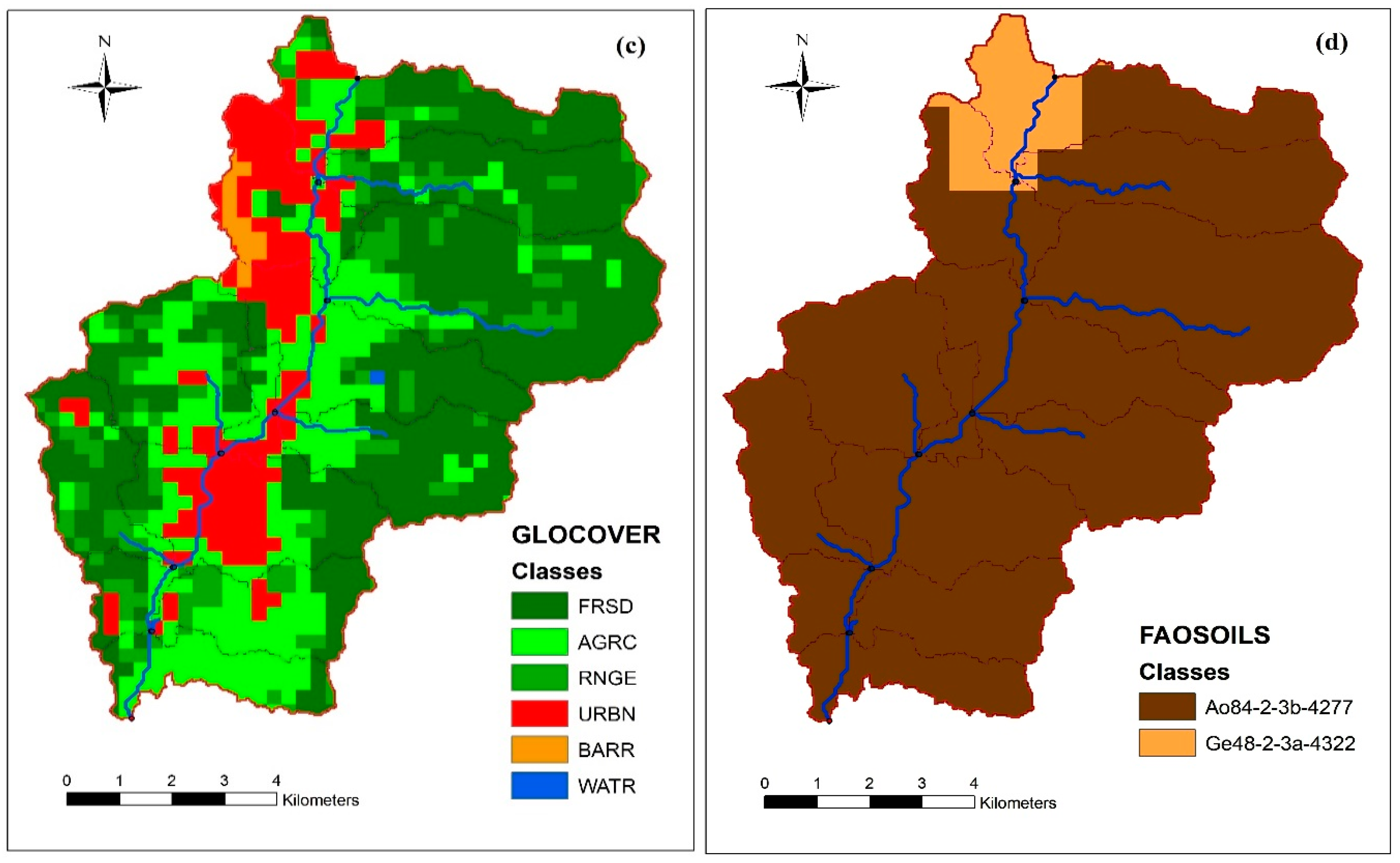
2.3. Data Preparation and Model Setup

In the study, the U.S. Geological Survey (USGS) Earth Explorer provided a resolution of 30 m of the digital elevation model (http://earthexplorer.usgs.gov/), the Global Land Cover Map 2009 utilized a 300-m land-use layer (http://due.esrin.esa.int/page_globcover.php), and a 10-km FAO v2 soil layer (http://www.fao.org/soils-portal/soil-survey/soil-maps-and-databases/faounesco-soil-map-of-the-world/en/) [49]. Historical weather data for 1979–2014 were obtained from the CFSR_World weather database on a daily basis. Meteorological Administration (KMA) provided weather data from 1993–2018 on a daily basis (https://web.kma.go.kr/eng/index.jsp). These weather stations (Figure 2a) provide daily wind velocity, solar radiation, minimum temperature, precipitation, and maximum temperature (

Table 1. Characteristics of the selected weather stations.

ID	Station	Latitude (Decimal Degree)	Longitude (Decimal Degree)	Elevation (m)
550	Osan	37.18787	127.04873	41.75
119	Suwon	37.25746	126.98300	39.81
549	Yongin	37.27011	127.22178	83

).

In the Osan watershed, the elevation varies between 1 and 351 m and the mean elevation is 67.25 m (Figure 2b). The watershed slope varies from 0.32–38.81%. The land-use dataset in Figure 2c shows that the watershed consists of FRSD (Forest; 47.02%), AGRC (Agriculture; 25.35%; mainly paddy rice), URBN (Urban Area; 14.21%), RNGE (Pasture; 12.06%), BARR (Barren lands; 1.09%), and WATR (Water; 0.09%). The soil dataset in Figure 2d indicates that the soil in the watershed is made up of Ge48-2-3a-4322 (Eutric Gleysols; 6.42%) and Ao48-2-3b-4277 (Orthic Acrisols; 93.58%) based on the Food and Agricultural Organization (FAO) soil classification.

The model demarcated the watershed into sub-basins, and threshold values for the soil, slope, and land use were set at 0% when defining the hydrological response units (HRUs) for the watershed. In order to maintain each landscape feature, a threshold of 0% was maintained in the model representation [50,51,52]. The model established 247 HRUs for 35 sub-basins, which was in accordance with the ratio range of 1–10 for HRUs and sub-basins suggested by the SWAT manual [53].

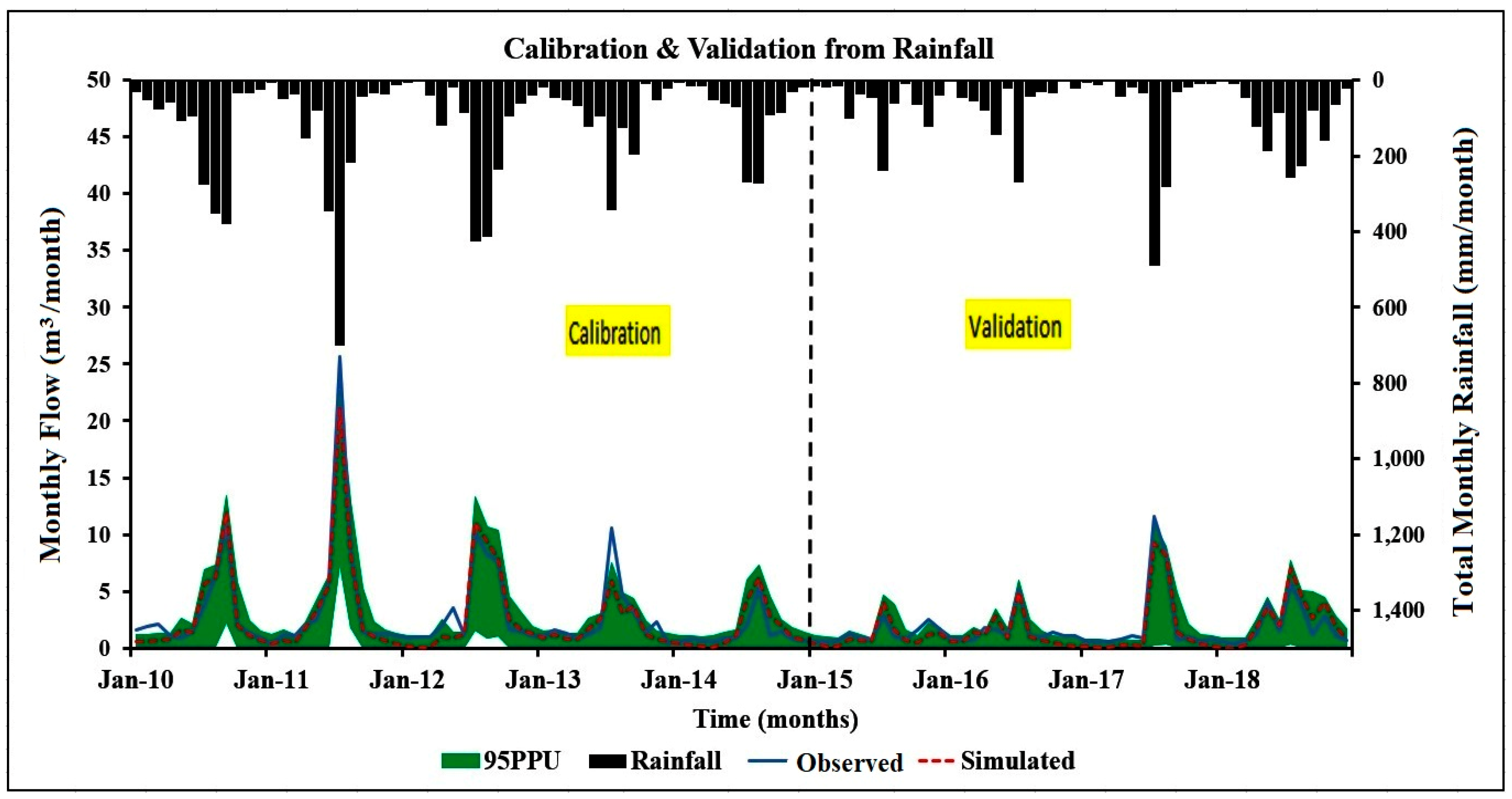
2.4. SWAT Model Evaluation

The SWAT calibration and uncertainty program (SWAT-CUP) software package provides a framework for decision-making integrating a semi-automated technique made up of sensitivity, calibration, and uncertainty analyses [54]. Observed monthly flow and simulated flow data from ArcSWAT were the model inputs. Generalized likelihood uncertainty estimation determined the sensitive parameters in SWAT-CUP [55] that were dependent on 25 established parameters for streamflow [11,56]. The model was calibrated using trial and error in comparing simulated and monthly observations until the model simulations satisfactorily matched the measured data [57,58,59].

Six objective functions were used in calibration and validation. Uncertainty analysis in SWAT-CUP was employed by the Sequential Uncertainty Fitting Version 2 (SUFI-2) method. The average output uncertainty of the Latin hypercube sample was determined by the 95 percent prediction uncertainty (95PPU) by the cumulative distribution rate at 2.5% and 97.5%. The p-factor is the 95PPU band proportion and the r-factor is a measure of the 95PPU band thickness. A simulation is deemed to correlate with the observed data at a point where the r-factor is nearest to zero and the p-factor is nearest to one. Theoretically, p-factors range between 0% and 100%, while r-factors range from 0 to infinity. SUFI-2 attempts to keep all of the data (i.e., a large p-factor, maximum of 100%) while minimizing the r-factor (minimum of 0). SUFI-2 first estimates parameters with a large variance within a theoretically justifiable range in order for the calculated data to immediately fall within 95PPU. This variance is subsequently reduced in stages while the p-factor and r-factor are tracked. Details are available in the manual [55,60,61,62].

The observed data for the watershed were separated into two datasets: 2010–2014 for calibration and 2015–2018 for validation. Details of the input/output for the hydrological parameters are shown in the manual [63]. In the model applicability, the following statistics were analyzed: p-factor and r-factor [55], percent bias (PBIAS) [64], root-mean-square error (RMSE; R²) [65], Nash–Sutcliffe model efficiency (NSE) [66], and RMSE-observation standard deviation ratio (RSR) [65]. Based on the discharge simulations, the monthly or daily model statistics were deemed acceptable if PBIAS < 15%, R² > 0.6, RSR ≤ 0.7, and NSE > 0.5 [60]. R² statistics for monthly streamflow were classified as follows: excellent (greater than or equal to 0.90), very good (between 0.75 and 0.89), good (between 0.50 and 0.74), fair (between 0.25 and 0.49), poor (between 0 and 0.24), and unsatisfactory (less than or equal to 0) [67]. The data for 2008–2009 (warm up period) were used for simulation, whereas 2010–2014 data were used for calibration, and 2015–2018 data were used for validation:

$$\mathit{PBIAS}=\left[\frac{{{\displaystyle \sum }}_{i=1}^n\left(Y_i{}^{obs}-Y_i{}^{sim}\right)\ast \left(100\right)}{{{\displaystyle \sum }}_{i=1}^n\left(Y_i{}^{obs}\right)}\right],$$

(2)

$$R^2=\left[\sqrt{\frac{1}{n}{{\displaystyle \sum }}_i^n{\left(Y_i{}^{sim}-Y_i{}^{obs}\right)}^2}\right],$$

(3)

$$\mathit{RSR}=\frac{RMSE}{STDE{V}_{obs}}=\left[\frac{\sqrt{{{\displaystyle \sum }}_{i=1}^n{\left(Y_i{}^{obs}-Y_i{}^{sim}\right)}^2}}{\sqrt{{{\displaystyle \sum }}_{i=1}^n{\left(Y_i{}^{obs}-Y_i{}^{mean}\right)}^2}}\right],$$

(4)

$$\mathit{NSE}=\mathit{1}-\left[\frac{{{\displaystyle \sum }}_{i=1}^n{\left(Y_i{}^{obs}-Y_i{}^{sim}\right)}^2}{{{\displaystyle \sum }}_{i=1}^n{\left(Y_i{}^{obs}-Y_i{}^{mean}\right)}^2}\right].$$

(5)

2.5. Downscaling and Bias Correction of Future Climate Data

Watershed models and GCMs can be used in examining climate change impacts on watershed hydrology. However, GCMs include major uncertainty, and the Intergovernmental Panel on Climate Change (IPCC; 2007) advises that the effects of multiple models and projections be included in research on climate change [68]. Statistical downscaling methods are thus essential for the long-term reliability of observed data sets representing base climate data. In the present study, precipitation (ppt), minimum temperature (Tmin), and maximum temperature (Tmax) were downscaled using observed data from 1993 to 2018. Typically, RCPs [69] and Special Report on Emissions Scenarios (SRES) [70] generate a variety of viable emission scenarios for climate projections.

The climate models in CMIP5 operate under four RCPs that provide daily climate projections (RCP 2.6, 4.5, 6.0, and 8.5) up to EC [71]. A total of 20 GCMs that included daily ppt, Tmax, and Tmin were selected by Eun and Cannon [72] and compared based on their ability to replicate extreme climate indices. The comparison was ranked by a group of experts (Expert Team on Climate Change Detection and Indices, ETCCDI) at the World Meteorological Organization [73]. Based on this finding, we selected the top 10 GCMs (

Table 2. Global climate models (GCMs) used for the study.

No.	Model Name	Model Expansion	Resolution (°)
1	CMCC-CM	Centro Euro-Mediterraneo sui Cambiamenti Climatici—Climate Model	0.750 × 0.748
2	CCSM4	Community Climate System Mode	1.250 × 0.942
3	CESM1-BGC	Community Earth System Model—Biogeochemical Model	1.250 × 0.942
4	CESM1-CAM5	Community Earth System Model—Community Atmospheric Model version 5	1.250 × 0.942
5	MRI-CGCM3	Meteorological Research Institute	1.125 × 1.122
6	CNRM-CM5	Centre National de Recherches Meteorologiques	1.406 × 1.401
7	HadGEM2-AO	Hadley Global Environment Model 2—Atmosphere Ocean	1.875 × 1.250
8	HadGEM2-CC	Hadley Global Environment Model 2—Carbon Cycle	1.875 × 1.250
9	HadGEM2-ES	Hadley Global Environment Model 2—Earth System	1.875 × 1.250
10	INM-CM4	Institute of Numerical Mathematics	2.000 × 1.500

). We used the RCP4.5 and RCP 8.5 scenarios. RCP 4.5 and 8.5 were selected because they represent a stable-end and a high-end climate change projection. These scenarios provide a wide range of long-term outcomes. RCPs do not have particular climate policy actions, hence they are suitable for use to explore a wide range of long-term outcomes. The RCP4.5 scenario assumes a world using technologies and strategies leading to stabilized radiative forcing before 2100 at 4.5 W/m². Contrariwise, in the RCP8.5 scenario, high population growth and a lack of highly developed technologies leads to radiative forcing reaching a high level, that is, 8.5 W/m² in 2100 [69].

For this downscaling process, a climate information production toolkit developed by the APEC climate center APCC Integrated Model Solution (AIMS) was used. This toolkit uses CMIP5 and CORDEX raw climate data for the downscaling of 29 GCMs for RCP 4.5 and 8.5 [74,75]. Depending on the project of interest, a user can either select a climate change or seasonal forecasting option in the AIMS software. The two data sources available for the project (CMIP5 and CORDEX) are coupled with the region of interest. Observed data is uploaded and evaluated with weather variables (e.g., ppt, Tmax and Tmin). GCMs models can be selected by the user to be downscaled for the observed, historical, and future periods under both scenarios. The selection of downscaling methods (SQM, SDQDM, and BCSA) using ETCCDI indices was also required [73]. In our study, a climate change project was run with the following ecosystem: water objective, CIMP5 data source, South Korea, observed data from the KMA, and SDQDM downscaling for RCP 4.5 and 8.5. Spatial correlations in temperature and precipitation to an acceptable degree were produced by the model [76]. Details of the QDM and SDQDM processes can be found in [72,77]. Details of the AIMS software are also available in its user manual, which can be freely downloaded (https://aims.apcc21.org/).

Daily ppt, Tmax, and Tmin data from 1976–2018 were used as the historical period and the 2006–2099 period data were available for future projections. The baseline, MC, and EC periods include 1993–2018, 2046–2065, and 2081–2099, respectively. Past research has reported average atmospheric CO₂ concentrations of 330, 540, and 940 ppm for the base period, RCP 4.5, and RCP 8.5, respectively, in the MC and EC periods [78,79,80]. To ensure that the model ran smoothly, a five-year warm-up period was established. A SWAT weather generator aided in simulating missing and unavailable data for wind velocity, solar radiation, and humidity for future projections [54]. Land cover was assumed not to change significantly as this has been addressed in other studies [10,14].

3. Results and Discussion

3.1. Model Evaluation

The calibration process aimed at minimizing variations among simulated and observed values. Five years (2010–2014) of monthly streamflow data were utilized for calibrating and four years (2015–2018) of data for validating the model. In the SWAT-CUP, parameters that were highly sensitive were identified for calibration using generalized likelihood uncertainty estimation. CN, ALPHA_BF, GW_DELAY, CH_K2, and SOL_AWC were the sensitive parameters as they directly affected streamflow (

Table 3. Model calibration parameters.

Parameter Identifier	Parameter	Detailed Parameter Description	Range	Fitted Value
r	CN2.mgt	SCS runoff curve number	0.1~0.5	0.2
v	ALPHA_BF.gw	Baseflow alpha factor	0~1	0.09
v	GW_DELAY.gw	Groundwater delay	10~30	24
v	CH_K2.rte	Alluvium main channel hydraulic conductivity	30~150	88
r	SOL_AWC.sol	The capacity of water available	±0.025	−0.08
v	GWQMN.gw	Shallow aquifer water threshold depth required to occur for the return flow	1000~3500	1591
v	GW_REVAP.gw	Coefficient of groundwater “revap”	±0.036	−0.01
v	ESCO.bsn	Compensation soil evaporation	0~1	0.69
v	REVAPMN.gw	Shallow aquifer water depth threshold required for return flow to occur	1~30	13
r	SOL_Z.sol	Soil surface to bottom layer depth	±0.025	0.04
r	SOL_K.sol	Saturated hydraulic conductivity	±0.025	0.03
v	EPCO.bsn	Compensation plant uptake factor	0~1	0.72
v	OV_N.hru	Overland flow for Manning’s number	±10	−1.23
v	RCHRG_DP.gw	Percolation fraction of deep aquifer	0~1	0.51
v	SFTMP.bsn	Temperature of snowfall	±20	−14
v	SMTMP.bsn	Temperature base of snow melt	±20	−10
v	SMFMX.bsn	Maximum yearly snow melting rate	0~20	5
v	SMFMN.bsn	Minimum yearly snow melting rate	0~20	17
v	TIMP.bsn	Temperature lag snow pack factor	0~1	0.35

Parameter identifiers in SWAT-CUP: ‘v’ stands for the model parameter value, which was replaced by a new value, and ‘r’ stands for the model parameter value, which was multiplied by a new value.

). The parameter identifier indicates the type of change made in order to calibrate the model whereas the range was the limit in which the parameters were adjusted in SWATCUP. The fitted value was achieved using trial and error until there was a good match between the simulated and observed values.

The shaded green regions in Figure 3 indicate the 95PPU. The p- and r-factors were both 0.88 in the calibration and 0.85 and 1.16 in the validation, respectively (

Table 4. Model statistics for calibration and validation.

Goodness of Fitness	Calibration	Validation
p-factor	0.88	0.85
r-factor	0.88	1.16
PBIAS	8.3	7.9
R2	0.91	0.88
NSE	0.91	0.88
RSR	0.30	0.36

). The model thus obtained satisfactory results. Other statistical metrics, namely PBIAS, R², NSE, and RSR, were evaluated. Their respective values were 8.3, 0.91, 0.91, and 0.30 for calibration, and 7.9, 0.88, 0.88, and 0.36 for validation. The performance indicators were also satisfactory [67].

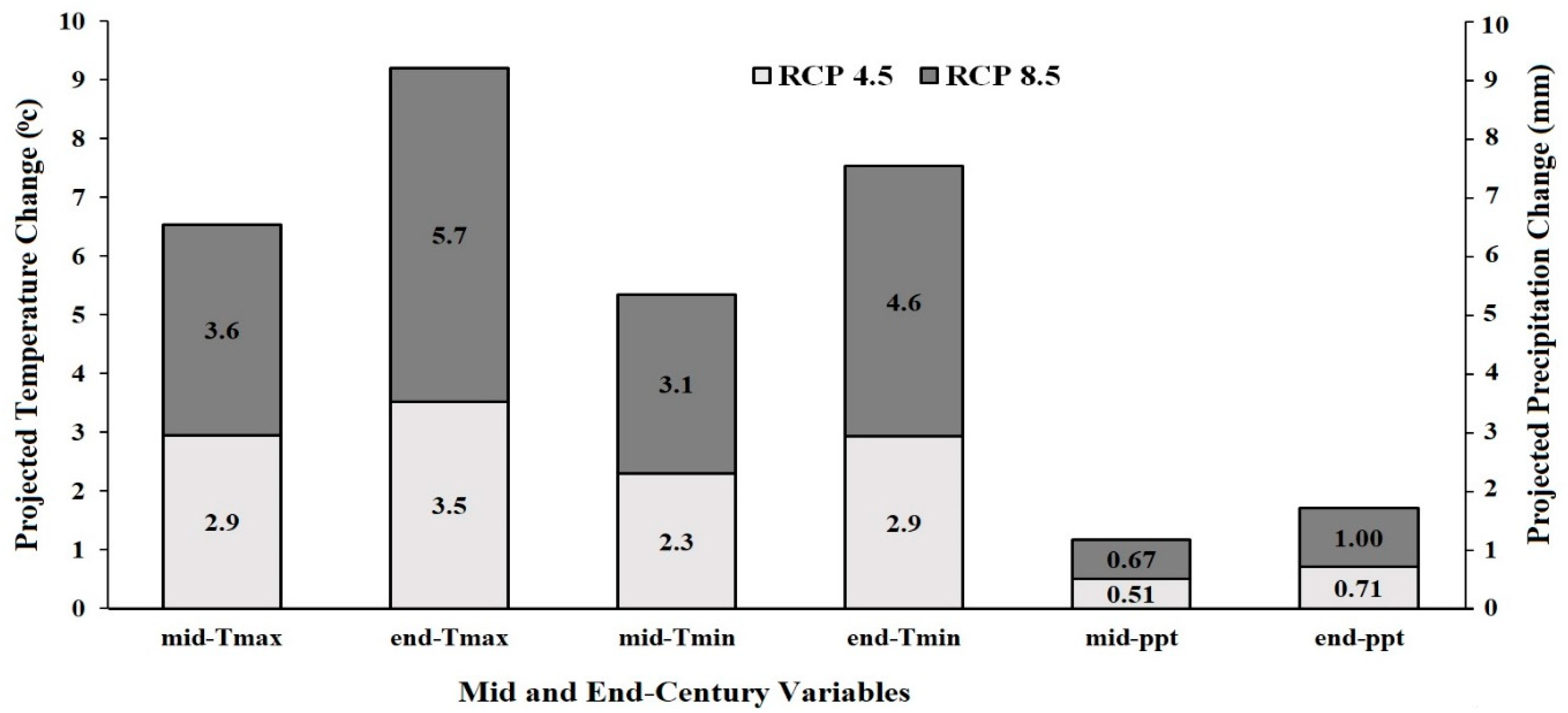
3.2. Projected Precipitation and Temperature

Precipitation increases were projected in the Osan watershed for the 10 GCMs used in the study. The average increase from the baseline period for all the GCMs was 0.51 mm (15.6%) in the MC period and 0.71 mm (21.7%) in the EC period under RCP 4.5 (Figure 4). RCP 8.5 predicted an increase of 0.67 (20%) and 1 mm (30.6%) in the MC and EC periods. Under RCP 4.5, precipitation exhibited the largest increase in HadGEM2-ES in both century periods, while the smallest increase was observed for CMCC-CM in the MC period and INM-CM4 in the EC period (Figure 5a). Under RCP 8.5, the highest increase was observed in MRI-CGCM3 in the MC period and CNRM-CM5 in the EC period, while the smallest increase was projected by INM-CM4 for both periods (Figure 5b).

Tmax and Tmin were also projected to rise in the future. Under the RCP 4.5 scenario, Tmax would rise by an average of 2.3 °C in the MC and by 2.9 °C for the EC period, whereas Tmin would increase by an average of 3.4 °C in the MC and in the EC period by 2.9 °C. Under RCP 8.5, Tmax would rise by 3.6 and 5.7 °C in the MC and EC periods, respectively, whereas Tmin would rise by 3.1 and 4.6 °C, respectively. Under RCP 4.5, the largest increase for Tmax and Tmin was observed for HadGEM2-ES in the MC and HadGEM2-CC in the EC, while the smallest increase was predicted by INM-CM4 for both periods. Under RCP 8.5, the increase in Tmax was highest for HadGEM2-CC and lowest for INM-CM4 in both periods, while Tmin increased the most for HadGEM2-CC in both periods and the least for INM-CM4 by the MC and HadGEM2-ES by the EC period. Multiple GCMs should be required for climate change impact studies to validate the results [34].

Temperature and precipitation in the Osan watershed will increase by approximately 2–5 °C and 15–30% in the MC and EC periods under both scenarios. Reports from the National Institute of Meteorological Research in 2009 predicted that temperatures will rise by 4 °C and precipitation will increase by 17% by 2100 [3], which is in close conformity with the projected results of this study. An increase in temperature may lead to longer cultivation periods and crop yields may also decrease due to water stress or a shift in water availability. Precipitation amounts greatly affect water resources and an increase in precipitation may lead to increased water spillage and possible flooding scenarios. Understanding these changes will aid decision makers to have a picture of the future scenarios, which may help in future climate change adaptation strategies.

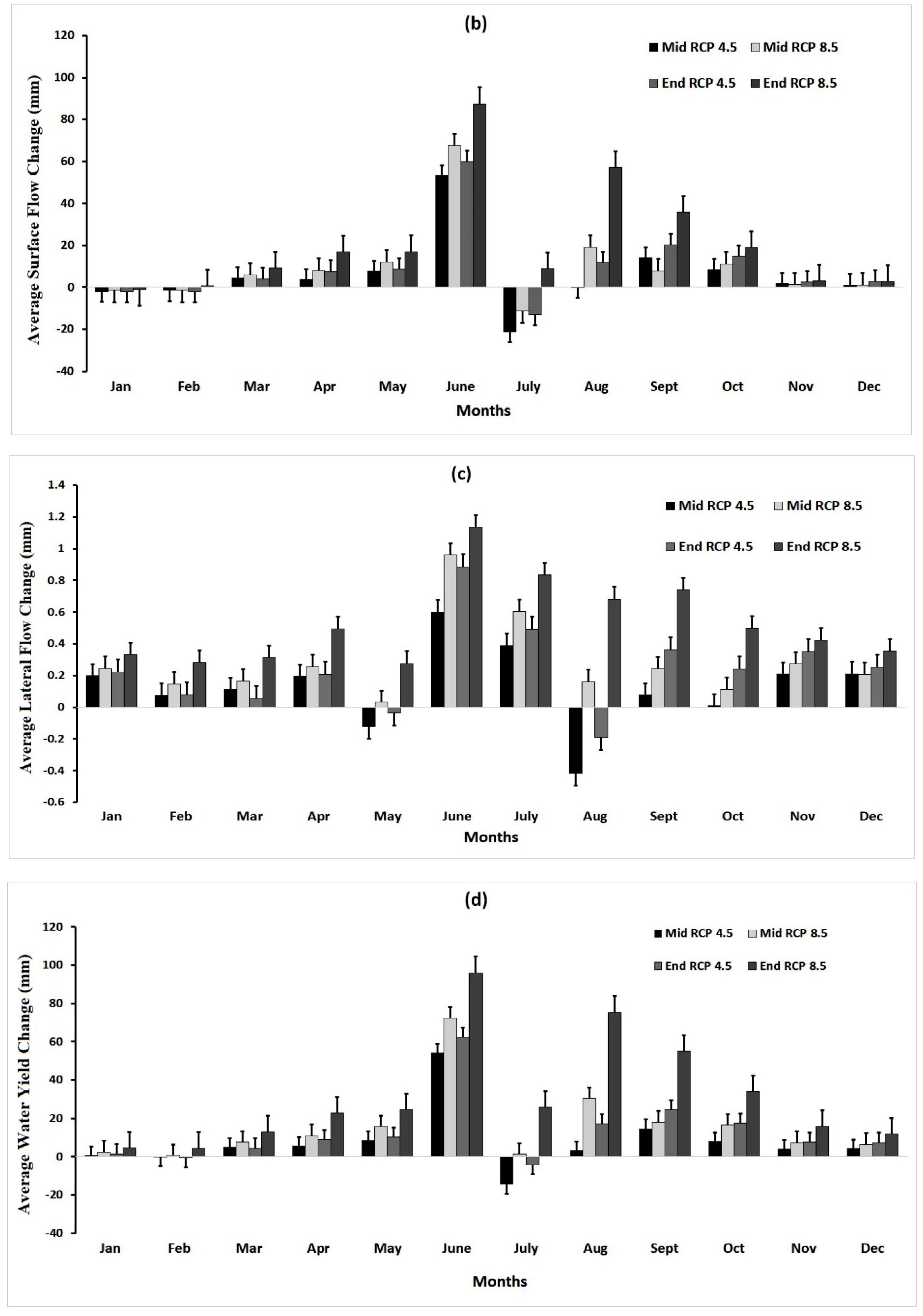
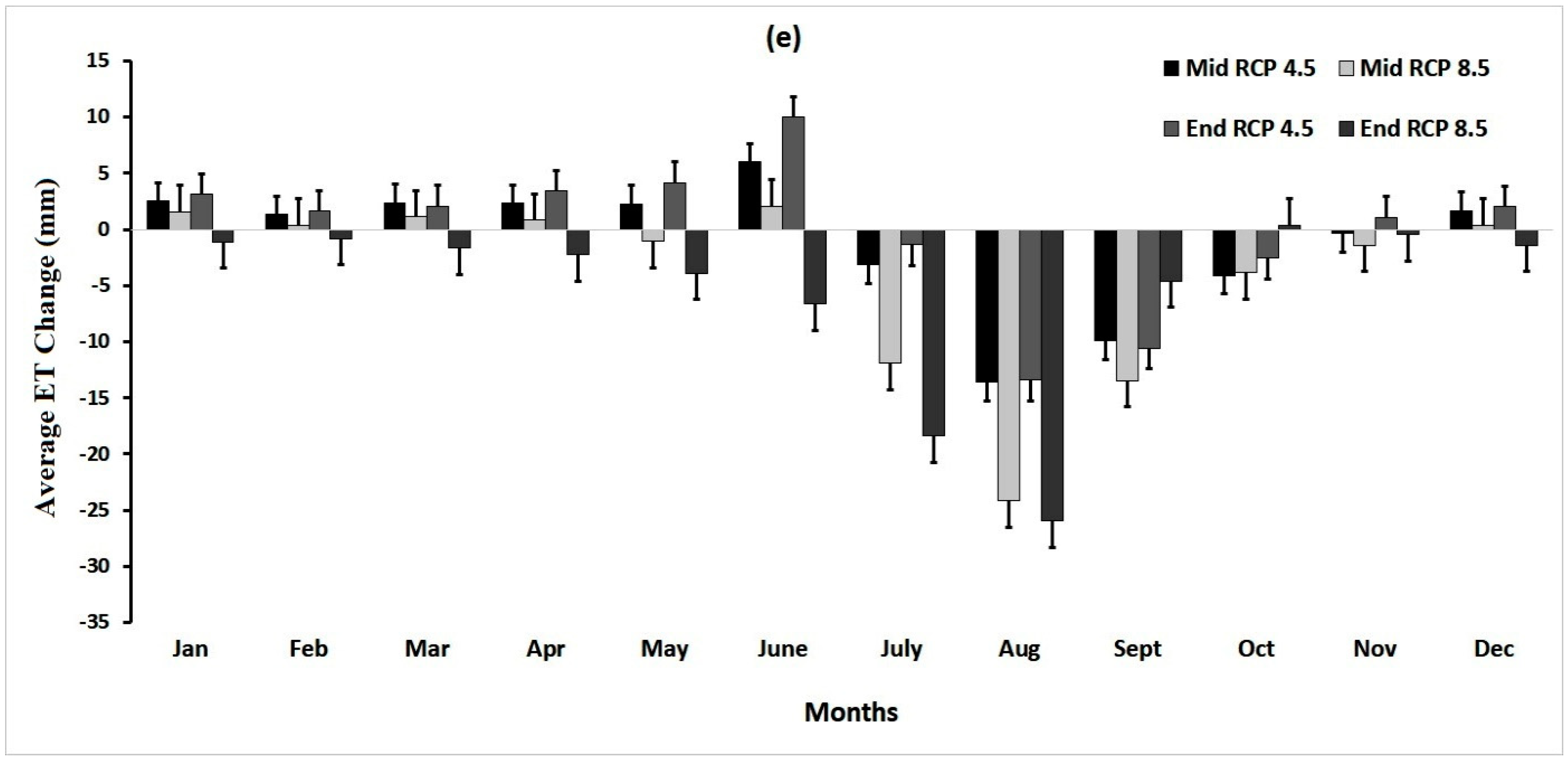
3.3. Monthly Climate Change Impact on Water Balance

Under RCP 4.5 and RCP 8.5 in the MC and EC periods from the baseline period, the future monthly water balance was also investigated for the Osan watershed. Figure 6 shows histograms and standard error bars for the water balance variable. Here, data uncertainty is clumped around the mean for all the simulated variables. Figure 6a shows that precipitation would increase from the baseline period in most months under both scenarios. Precipitation would decline in the MC period in January, February, and July and in the EC in February and July under RCP 4.5. Precipitation would also decrease in February and July for the MC period whereas only in July for the EC period under RCP 8.5. The largest increase in precipitation under RCP 4.5 was in June, with increases of 72.84 (57%) and 88.67 mm (69.3%) for both MC and EC periods, respectively. Precipitation mostly increased in June under RCP 8.5, by 95.75 (74.8%) and 114.99 mm (89.8%), respectively. The largest precipitation decline under RCP 4.5 was in July (42.18 mm [11%] and 29.21 mm [7.6%] for MC and EC periods, respectively). The highest precipitation decrease under RCP 8.5 was also in July, with 33.1 mm (8.6%) for the MC period and 9.25 mm (2.4%) for the EC period.

South Korea’s monsoons normally occur between June and August, delivering about 60–70% of the annual total rainfall. The results for both periods indicated a significant rise in precipitation in June and a slight decrease in July under both scenarios. Fluctuations of the precipitation increase in June and decrease in July may be due to a shift in the monsoon season as it starts earlier than usual. The summer monsoon in Korea has two peaks in sub seasonal rainfall structures from late June to mid-July and from mid-August to early September [81]. High atmospheric CO₂ concentrations in the RCP4.5 and RCP8.5 scenario (540 and 940 ppm for both mid-century and end-century compared to 330 ppm for baseline) used in the study may be the main reason for the changes as atmospheric CO₂ is expected to increase in the future. This may cause floods in June and droughts in July, thus affecting rain-fed crops and possibly leading to the destruction of property because 80% of Korea consists of hills [27]. A shift in future precipitation is likely to affect agriculture because the planting and harvesting periods may change.

Surface flow also increased in most months for both periods under both scenarios (Figure 6b). Under RCP 4.5, the surface flow decreased in January, February, July, and August for the MC period and in January, February, and July for the EC period. Under RCP 8.5, surface flow decreased in January, February, and July for the MC period and only in January for the EC period. The largest increase in surface flow under RCP 4.5 was in June with 53.19 (117.3%) and 59.89 mm (132%) in the MC and EC periods. Under RCP 8.5, the largest increase occurred in June: 67.41 (148.6%) and 87.51 mm (192.9%) for the MC and EC periods, respectively. The largest surface flow decrease under RCP 4.5 was 21.09 (10.5%) and 12.95 mm (6.4%) for July in the MC and EC periods, while the largest decrease under RCP 8.5 was in July in the MC period (11.09 mm; 5.5%) and January in the EC period (1.13 mm; 23.4%). Because precipitation increased and decreased in June and July, respectively, surface runoff also increased and decreased in the same months because surface runoff depends on precipitation.

Lateral flow exhibited a similar pattern to the other water balance variables, increasing in most months for both periods under both scenarios (Figure 6c). Total lateral flow was projected to decrease in May and August in both periods under RCP 4.5 but increase under RCP 8.5. The highest lateral flow increase under RCP 4.5 was in June, with 0.6 mm (43%) for the MC period and 0.89 mm (63.5%) in the EC; under RCP 8.5, June also exhibited the highest increase, with 0.96 (68.6%) and 1.13 mm (81%), respectively. The largest decrease in lateral flow under RCP 4.5 was 0.12 mm (7.2%) for the MC period and 0.04 mm (2%) for the EC period in May; under RCP 8.5, the largest decrease was 0.03 (1.9%) and 0.28 mm (16%), respectively, in the same month.

Water yield was predicted to decrease in February and July under RCP 4.5, whereas it would rise under RCP 8.5 for both periods. The largest increase in the water yield under RCP 4.5 was in June, with 54.13 (100.6%) and 62.41 mm (115.9%) for the MC and EC periods, respectively. June also saw the largest rise in water yield under RCP 8.5 (72.4 [134.5%] and 96.1 mm [178.5%], respectively). The largest decrease in the water yield from the baseline period under RCP 4.5 was 14.59 mm (6.6%) for the MC period and 4.24 mm (1.9%) for the EC period, both in July. The smallest increase in water yield under RCP 8.5 was in February, with 0.74 mm (9.6%) in the MC period and 4.4 mm (57.4%) in the EC period (Figure 6d).

ET was predicted to decrease from June to November and slightly fluctuate in the other months for both periods under both RCP scenarios (Figure 6e). The largest increase in ET was in June under RCP 4.5 (6 mm [8.1%] for the MC period and 9.98 mm [13.4%] for the MC period). The largest increase in ET under RCP 8.5 was in June for the MC period (2.1 mm; 2.7%) and in October for the EC period (0.38 mm; 1.2%). The largest decrease in ET under RCP 4.5 was in August, with 13.6 (12.4%) and 13.41 mm (12.2%) in the EC periods, respectively. The smallest increase in ET under RCP 8.5 was also in August, with 24.16 (22%) and 25.94 mm (23.6%), respectively. The larger ET decrease in July–October was due to decreases in transpiration caused by an increased atmospheric CO₂ concentration. Plant activities play a major role in ET during this period when plants are actively developing [82].

3.4. Impact of Climate Change on Annual Water Balance

Results from the SWAT model for the annual water balance under the RCP 4.5 and 8.5 scenarios for the MC and EC periods are shown on

Table 5. Average annual water balance for mid-century (MC; 2046–2065) and end-century (EC; 2081–2099) under RCP 4.5 and 8.5 from baseline (1993–2018).

Variable	Baseline (mm)	MC RCP 4.5 (mm)	MC RCP 8.5 (mm)	EC RCP 4.5 (mm)	EC RCP 8.5 (mm)
Precipitation	1293.7	1374.96 (81.26)	1433.07 (139.37)	1451 (157.3)	1596.12 (302.42)
Surface Flow	524.64	594.88 (70.24)	644.76 (120.11)	640.07 (115.43)	781.86 (257.22)
Water Yield	689.89	783.44 (93.55)	879.81 (189.92)	846.33 (156.44)	1073.17 (383.28)
Lateral Flow	21.41	22.95 (1.54)	24.83 (3.42)	24.33 (2.92)	27.77 (6.36)
Evapotranspiration	582	569.32 (−12.68)	532.5 (−49.5)	581.52 (−0.48)	502.58 (−79.42)

. These results would be of use in projecting future water availability within the Osan watershed. Precipitation would increase for both periods under both scenarios: 6.2% in the MC and 12.2% in the EC periods under RCP 4.5 and 10.7% for the MC and 23.4% for the EC periods under RCP 8.5. Similarly, the surface flow would increase for both periods and both scenarios. Under RCP 4.5, the surface flow increased by 13.4% and 22.0% and, under RCP 8.5, it increased by 22.9% and 49.0% in the MC and EC periods, respectively.

Water yield within the Osan watershed also increased in all cases: 13.6% in the MC period and 22.7% in the EC period under RCP 4.5 and 27.5% in the MC period and 55.6% in the EC period under RCP 8.5. Lateral flow would increase for both periods and both scenarios: 7.2% and 13.6% for the MC and EC periods, respectively, under RCP 4.5 and 16.0% and 29.7% for the MC and EC periods, respectively, under RCP 8.5.

ET was predicted to decrease from baseline for both periods and scenarios. ET decreased by 2.2% and 0.1% in the MC and EC periods, respectively, under RCP 4.5 and by 8.5% and 13.6% in the MC and EC periods, respectively, under RCP 8.5. This may be due to the high atmospheric CO₂ concentrations used in the RCP 4.5 and 8.5 scenarios (540 ppm for the MC and 940 ppm for the EC periods with respect to 330 ppm as the baseline). Transpiration decreases as the atmospheric CO₂ concentration increases due to plants having efficient water use [10,83,84,85]. On the other hand, evaporation depends mainly on temperature and water availability.

The results thus revealed that precipitation, surface flow, lateral flow, and water yield would increase while ET would decrease in the Osan watershed in the MC and EC periods for both RCPs 4.5 and 8.5. This is expected as a result of an increase in precipitation in the region; thus, as precipitation increases, ET decreases, and as precipitation decreases, ET increases. The differences in precipitation and temperature that would drive more ET are outweighed by atmospheric CO₂ concentration changes. Hence, a large decrease in transpiration will result in a decrease in ET. Transpiration plays a key role in the water cycle, especially in our area of study, which is predominantly made up of cultivated crops and forest cover [10]. These results are similar to a Ministry of Environment report in 2018, which predicted the average precipitation in seven major domestic areas compared to the past three decades (1976–2005), projecting a 14.8% increase in the early 21st century (2011–2040), a 17.1% increase by the mid-21st century (2071–2100), and an 11.4% increase by the late 21st century (2071–2100) [86]. In accordance with these projections, floods and other weather-related disasters were estimated to occur more frequently [87,88]. Due to an increase in precipitation, flooding will also increase the surface flow, thus raising the risk of landslides and affecting water leakage and water recharge. Climate change will likely influence water quality as a rise in water temperature would affect water ecosystems [89]. In combatting the negative climate change effects on water resources, adaptation strategies are required, such as dam construction and improved dam/reservoir operating methods, in the region [90,91].

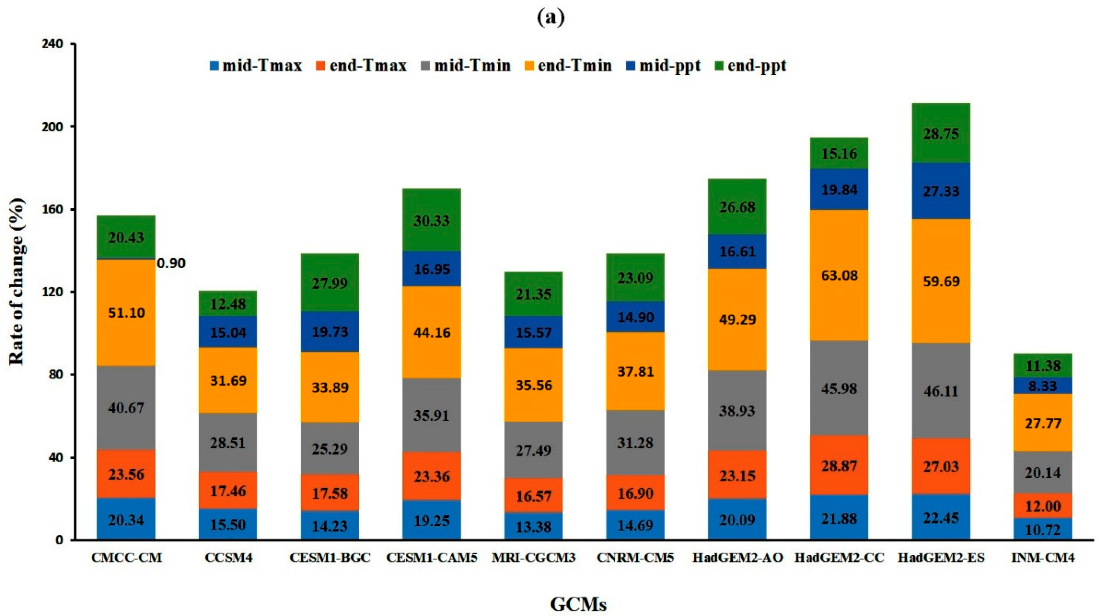
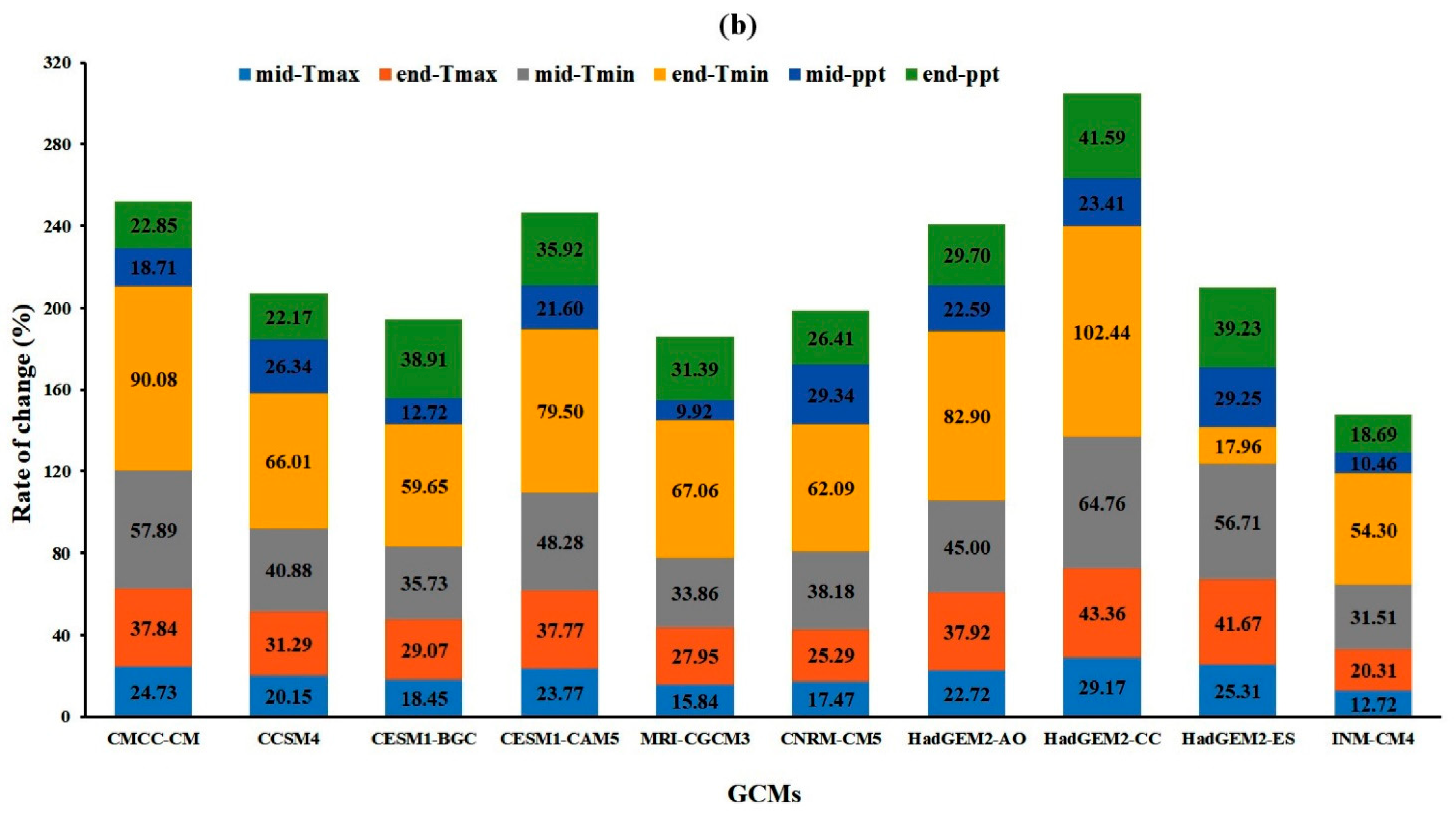
3.5. GCMs Variability

Investigating the differences in the water balance predicted by the individual GCMs under the RCP 4.5 and 8.5 scenarios for the MC and EC periods are essential for identifying the degree to which changes in climate would influence water availability in the Osan watershed (

Table 6. Variability amongst the 10 GCMs used in the study.

Scenario	GCMs	Precipitation (mm)		Surface Flow (mm)		Water Yield (mm)		Lateral Flow (mm)		ET (mm)
		MC	EC	MC	EC	MC	EC	MC	EC	MC	EC
	CMCC-CM	−141.8	128.1	−119.62	86.78	−161.28	83.89	−2.04	1.02	19.1	41.7
	CCSM4	99.5	80.5	66.22	67.31	82.74	77.92	1.6	0.99	13.1	7.7
	CESM1-BGC	179.2	188	141.18	123.47	203.91	192.38	3.57	4.4	−23.1	−8.3
	CESM1-CAM5	123.4	297.3	93.76	217.16	128.71	277.66	2.26	4.33	−5.1	19.2
RCP 4.5	MRI-CGCM3	8.2	108.3	−4.38	75.69	−2.54	81.24	0.58	1.14	9.1	25.8
	CNRM-CM5	66.4	252.4	52.42	172.41	76.33	257.09	1.18	5.32	−9.2	−7.1
	HadGEM2-AO	181.8	225.5	149.14	147.1	205.49	229.02	3.45	5.55	−21.7	−4.4
	HadGEM2-CC	22.2	22.2	28.21	28.21	46.62	46.62	1.24	1.24	−22.5	−22.5
	HadGEM2-ES	248.2	262	234.47	198.16	268	262.61	2.7	4.63	−26.6	−5.5
	INM-CM4	25.5	8.7	60.95	37.97	87.52	55.93	0.84	0.54	−59.9	−51.4
	CMCC-CM	37.1	196.9	29.95	206.5	21.68	270.24	-0.06	2.66	17	−69
	CCSM4	208.2	159.8	215.82	148.01	295.73	225.79	3.25	3.68	−84.2	−66.5
	CESM1-BGC	45.7	444	35.03	370.68	66.95	520.17	1.75	7.94	−21.8	−78.9
	CESM1-CAM5	142.6	276.8	126.58	232.68	224.41	347.01	4.44	5.89	−78	−68.9
RCP 8.5	MRI-CGCM3	−6.7	366.9	16.65	278.38	83.09	437.51	2.16	8.5	−87.4	−71.8
	CNRM-CM5	345.5	128.4	260.68	120.19	359.82	212.69	5.92	4.03	−18.2	−81.4
	HadGEM2-AO	175.3	271.4	154.53	208.91	258.58	349.22	4.87	7.39	−83.8	−77.4
	HadGEM2-CC	191.9	443.2	132.59	367.58	202.23	504.45	4.56	7.6	−12.3	−59.2
	HadGEM2-ES	139.7	608.3	142.86	533.89	224.56	729.03	3.35	9.94	−77.6	−117.7
	INM-CM4	114.4	128.5	86.46	105.41	162.11	236.69	3.97	5.99	−48.7	−103.4

‘MC’ represents mid-century and ‘EC’ represents end-century.

). Under RCP 4.5, precipitation increased within all GCMs for both periods except for CMCC-CM in the MC period, which predicted a considerable decline. In addition, water yield and surface water were expected to increase as the precipitation increased. Water yield and surface water increased for both periods for all GCMs with the exceptions of CMCC-CM and MRI-CGCM3, which predicted a decrease in the MC period. Lateral flow increased in all GCMs in both periods except for CMCC-CM. ET decreased in all GCMs in both periods except for CMCC-CM and CCSM4, which predicted 1.5% and 1.3% increases in the MC period and 3.2% and 0.6% increases in the EC period.

Under RCP 8.5, precipitation increased within all GCMs for both periods with the exception of MRI-CGCM3, which decreased by 0.5%. Surface flow also increased in all GCMs for both periods, with the largest increase of 49.7% observed in CNRM-CM5 in the MC period and 101.7% in HadGEM2-ES for the EC period. In all periods, water yield increased in all GCMs, with the largest increase in CNRM-CM5 in the MC period (52.2%) and in HadGEM2-ES in the EC period (105.6%). Lateral flow increased in all GCMs for both periods except a decrease of 0.3% in CMCC-CM in the MC period. ET decreased for all GCMs for both periods, with the largest decrease of 15% for MRI-CGCM3 in the MC and of 20.2% for HadGEM2-ES in the EC period. The only exception was a slight increase of 2.9% for CMCC-CM in the MC period.

4. Conclusions

Future climate change impacts on the water balance were assessed using the SWAT model in the Osan watershed, South Korea. On a daily time-step, the model was calibrated using six statistic metrics. Model calibration and validation were satisfactory. Ten GCMs were used to predict these impacts from 2046–2065 (MC) and 2081–2099 (EC) periods from a baseline period of 1993–2018 under RCPs 4.5 and 8.5.

We projected hotter and wetter future conditions using the 10 downscaled GCMs. This occurs as a result of an increase in temperature and precipitation for both MC and EC under the RCP 4.5 and 8.5 scenarios when compared to the baseline. Monthly precipitation, surface flow, lateral flow, and water yield will rise in the month of June and a decline in July during the summer monsoon season in the future. The atmospheric CO₂ concentration increase leads to a decrease in ET for the MC and EC period under the RCP 4.5 and 8.5 scenarios. This may be a result of a higher atmospheric moisture demand due to an increase in temperature. Similarly, annual precipitation, surface flow, lateral flow, and water yield was projected under RCP 4.5 and 8.5 for the two periods. These increases would significantly affect the water balance in the Osan watershed, where storms and floods may occur with greater frequency. Annual ET was expected to decline in the MC and EC period under both scenarios. This is expected as a result of an increase in precipitation; thus, as precipitation increases, ET decreases and vice versa. These findings were consistent with other studies in the region.

Overall, the Osan watershed will experience wetter conditions in the future, which may make it vulnerable to floods if not adequately managed. Summer monsoon rains may fluctuate more sharply, with heavy rains in June, lower rainfall in July, and more rain in the late summer, leading to the possibility of both flooding and drought in the future. This would provide a major challenge in the management and planning of water resources.

In the present study, we did not consider potential land-use changes or human-related activities. Further research in this regard is necessary for decision-makers to efficiently manage the water resources within the watershed. However, the study’s results improve the understanding of climate change impacts on the Osan watershed under various climate change scenarios in the future.

References

1. Hagemann, S.; Chen, C.; Clark, D.B.; Folwell, S.; Gosling, S.N.; Haddeland, I.; Hanasaki, N.; Heinke, J.; Ludwig, F.; Voss, F.; et al. Climate change impact on available water resources obtained using multiple global climate and hydrology models. Earth Syst. Dyn. 2013, 4, 129–144. [Google Scholar] [CrossRef] [Green Version]
2. Zhang, A.; Zhang, C.; Fu, G.; Wang, B.; Bao, Z.; Zheng, H. Assessments of impacts of climate change and human activities on runoff with SWAT for the Huifa River Basin, Northeast China. Water Resour. Manag. 2012, 26, 2199–2217. [Google Scholar] [CrossRef]
3. Edenhofer, O.R.; Pichs-Madruga, Y.; Sokona, E.; Farahani, S.; Kadner, K.; Seyboth, A.; Adler, I.; Baum, S.; Brunner, P.; Eickemeier, B.; et al. (Eds.) IPCC: Summary for Policymakers. In Climate Change 2014: Mitigation of Climate Change. Contribution of Working Group III to the Fifth Assessment Report of the Intergovernmental Panel on Climate Change; Cambridge University Press: Cambridge, UK; New York, NY, USA, 2014. [Google Scholar]
4. National Institute of Meteorological Research (NIMR). Understanding of Climate Change II.; NIMR: Seoul, Korea, 2009; 611p.
5. National Institute of Meteorological Research (NIMR). The Application of Regional Climate Change Scenario for the National Climate Change (IV); NIMR: Seoul, Korea, 2008; 355p.
6. Ministry of Land, Infrastructure and Transport. Nation-Wide River Basins Investigation Report; MOLIT: Seoul, Korea, 2012.
7. Ministry of Land, Infrastructure and Transport. The 4th Long-Term Comprehensive Plan of Water Resources (2001–2020); 3rd Revision; K-Water, MOLIT: Seoul, Korea, 2016.
8. Pradhanang, S.M.; Mukundan, R.; Schneiderman, E.M.; Zion, M.S.; Anandhi, A.; Pierson, D.C.; Frei, A.; Easton, Z.M.; Fuka, D.; Steenhuis, T.S. Streamflow responses to climate change: Analysis of hydrologic indicators in a New York City water supply watershed. JAWRA J. Am. Water Resour. Assoc. 2013, 49, 1308–1326. [Google Scholar] [CrossRef]
9. Jeung, S.J.; Sung, J.H.; Kim, B.S. Assessment of the impacts of climate change on climatic zones over the Korean Peninsula. Adv. Meteorol. 2019, 1–11. [Google Scholar] [CrossRef] [Green Version]
10. Ercan, M.B.; Maghami, I.; Bowes, B.D.; Morsy, M.M.; Goodall, J.L. Estimating potential climate change effects on the upper neuse watershed water balance using the SWAT model. JAWRA J. Am. Water Resour. Assoc. 2020, 56. [Google Scholar] [CrossRef]
11. Arnold, J.G.; Srinivasan, R.; Muttiah, R.S.; Williams, J.R. Large-area hydrologic modeling and assessment: Part I. Model development. J. Am. Water Resour. Assoc. 1998, 34, 73–89. [Google Scholar] [CrossRef]
12. Abbaspour, K.C.; Rouholahnejad, E.; Vaghefi, S.; Srinivasan, R.; Yang, H.; Kløve, B. A continental-scale hydrology and water quality model for Europe: Calibration and uncertainty of a high-resolution large-scale SWAT model. J. Hydrol. 2015, 524, 733–752. [Google Scholar] [CrossRef] [Green Version]
13. Uniyal, B.; Jha, M.K.; Verma, A.K. Assessing climate change impact on water balance components of a river basin using SWAT model. Water Resour. Manag. 2015, 29, 4767–4785. [Google Scholar] [CrossRef]
14. Bhatta, B.; Shrestha, S.; Shrestha, P.K.; Talchabhadel, R. Evaluation and application of a SWAT model to assess the climate change impact on the hydrology of the Himalayan River Basin. CATENA 2019, 181, 104082. [Google Scholar] [CrossRef]
15. Yan, T.; Bai, J.; Toloza, A.; Liu, J.; Shen, Z. Future climate change impacts on streamflow and nitrogen exports based on CMIP5 projection in the Miyun Reservoir Basin, China. Ecohydrol. Hydrobiol. 2018. [Google Scholar] [CrossRef]
16. Park, J.-Y.; Yu, Y.-S.; Hwang, S.-J.; Kim, C.; Kim, S.-J. SWAT modeling of best management practices for Chungju dam watershed in South Korea under future climate change scenarios. Paddy Water Environ. 2014, 12, 65–75. [Google Scholar] [CrossRef]
17. Ahn, S.R.; Jeong, J.H.; Kim, S.J. Assessing drought threats to agricultural water supplies under climate change by combining the SWAT and MODSIM models for the Geum River basin, South Korea. Hydrol. Sci. J. 2015, 61, 2740–2753. [Google Scholar] [CrossRef] [Green Version]
18. Park, J.Y.; Park, G.A.; Kim, S.J. Assessment of future climate change impact on water quality of Chungju Lake, South Korea, using WASP coupled with SWAT. JAWRA J. Am. Water Resour. Assoc. 2013, 49, 1225–1238. [Google Scholar] [CrossRef]
19. Shope, C.L.; Maharjan, G.R.; Tenhunen, J.; Seo, B.; Kim, K.; Riley, J.; Arnhold, S.; Koellner, T.; Ok, Y.S.; Peiffer, S.; et al. Using the SWAT model to improve process descriptions and define hydrologic partitioning in South Korea. Hydrol. Earth Syst. Sci. 2014, 18, 539–557. [Google Scholar] [CrossRef] [Green Version]
20. Ahn, S.R.; Kim, S.J. Analysis of water balance by surface–groundwater interaction using the SWAT model for the Han River basin, South Korea. Paddy Water Environ. 2018. [Google Scholar] [CrossRef]
21. Lee, K.S.; Chung, E.-S. Hydrological effects of climate change, groundwater withdrawal, and land use in a small Korean watershed. Hydrol. Process. 2007, 21, 3046–3056. [Google Scholar] [CrossRef]
22. Lee, J.; Jung, C.; Kim, S.; Kim, S. Assessment of climate change impact on future groundwater-level behavior using SWAT groundwater-consumption function in Geum River Basin of South Korea. Water 2019, 11, 949. [Google Scholar] [CrossRef] [Green Version]
23. Kim, S.J.; Jun, H.D.; Kim, B.S.; Kim, H.S. Evaluation of climate change impacts on the water resource system of the Han-River Basin in South Korea for the AR4 SRES A2 Scenario. Hydrol. Days 2010. [Google Scholar] [CrossRef]
24. Park, J.Y.; Park, M.J.; Ahn, S.R.; Park, G.A.; Yi, J.E.; Kim, G.S.; Srinivasan, R.; Kim, S.J. Assessment of future climate change impacts on water quantity and quality for a mountainous dam watershed using SWAT. Trans. ASABE 2011, 54, 1725–1737. [Google Scholar] [CrossRef]
25. Kim, J.; Choi, J.; Choi, C.; Park, S. Impacts of changes in climate and land use/land cover under IPCC RCP scenarios on streamflow in the Hoeya River Basin, Korea. Sci. Total Environ. 2013, 452–453, 181–195. [Google Scholar] [CrossRef]
26. Kim, S.; Noh, H.; Jung, J.; Jun, H.; Kim, H.S. Assessment of the impacts of global climate change and regional water projects on streamflow characteristics in the Geum River Basin in Korea. Water 2016, 8, 91. [Google Scholar] [CrossRef] [Green Version]
27. Joh, H.-K.; Lee, J.-W.; Park, M.-J.; Shin, H.-J.; Yi, J.-E.; Kim, G.-S.; Srinivasan, R.; Kim, S.-J. Assessing climate change on hydrological components of a small forest watershed through SWAT calibration of evapotranspiration and soil moisture. Trans. ASABE 2011, 54, 1773–1781. [Google Scholar] [CrossRef]
28. Nkomozepi, T.; Chung, S.-O. The effects of climate change on the water resources of the Geumho River Basin, Republic of Korea. J. Hydro-Environ. Res. 2014, 8, 358–366. [Google Scholar] [CrossRef]
29. Maloney, E.D.; Camargo, S.J.; Chang, E.; Colle, B.; Fu, R.; Geil, K.L.; Hu, Q.; Jiang, X.; Johnson, H.; Karnauskas, K.B.; et al. North American climate in CMIP5 experiments: Part III: Assessment of twenty-first-century projections. J. Clim. 2014, 27, 2230–2270. [Google Scholar] [CrossRef]
30. Jenkins, G.; Lowe, J. Handling Uncertainties in the UKCIP02 Scenarios of Climate Change; Hadley Centre Technical Note 44; Met Office: Exeter, UK, 2003.
31. Murphy, J.M.; Sexton, D.M.H.; Barnett, D.N.; Jones, G.S.; Webb, M.J.; Collins, M.; Stainforth, D.A. Quantification of modelling uncertainties in a large ensemble of climate change simulations. Nature 2004, 430, 768–772. [Google Scholar] [CrossRef] [PubMed]
32. Mizuta, R.; Oouchi, K.; Yoshimura, H.; Noda, A.; Katayama, K.; Yukimoto, S.; Hosaka, M.; Kusunoki, S.; Kawai, H.; Nakagawa, M. 20-km-mesh global climate simulations using JMA-GSM model—Mean climate states. J. Meteorol. Soc. Jpn. 2006, 84, 165–185. [Google Scholar] [CrossRef] [Green Version]
33. Christensen, J.H.; Carter, T.; Rummukainen, M.; Amanatidis, G. Evaluating the performance and utility of regional climate models in climate change research: Reducing uncertainties in climate change projections—The PRUDENCE approach. Clim. Chang. 2007, 81 (Suppl. 1), 1–6. [Google Scholar] [CrossRef]
34. Arnell, N.W. Climate change and global water resources: SRES emissions and socio-economic scenarios. Glob. Environ. Chang. 2004, 14, 31–52. [Google Scholar] [CrossRef]
35. Lee, K.S. Rehabilitation of the hydrologic cycle in the anyangcheon watershed. In Sustainable Water Resources Research Center of 21st Century Frontier Research Program; Seoul National University: Seoul, Korea, 2005. (In Korean) [Google Scholar]
36. Bae, D.H.; Jung, I.W.; Chang, H. Potential changes in Korean water resources estimated by high-resolution climate simulation. Clim. Res. 2008, 35, 213–226. [Google Scholar] [CrossRef]
37. Jung, I.W.; Bae, D.H.; Lee, B.J. Possible change in Korean streamflow seasonality based on multi-model climate projections. Hydrol. Process. 2012. [Google Scholar] [CrossRef]
38. Kim, K.; Kim, B.; Eum, J.; Seo, B.; Shope, C.L.; Peiffer, S. Impacts of land use change and summer monsoon on nutrients and sediment exports from an agricultural catchment. Water 2018, 10, 544. [Google Scholar] [CrossRef] [Green Version]
39. Ashu, A.; Lee, S.-I. Reuse of agriculture drainage water in a mixed land-use watershed. Agronomy 2019, 9, 6. [Google Scholar] [CrossRef] [Green Version]
40. Eckhardt, K.; Fohrer, N.; Frede, H.-G. Automatic model calibration. Hydrol. Process. 2005, 19, 651–658. [Google Scholar] [CrossRef]
41. Neitsch, S.L.; Arnold, J.R.; Kiniry, J.R.; Williams, J.R. Soil and Water Assessment Tool Theoretical Documentation; Version 2005; Soil and Water Research Laboratory, Blackland Research Center: Temple, TX, USA, 2005.
42. Gassman, P.W.; Reyes, M.R.; Green, C.H.; Arnold, J.G. The soil and water assessment tool: Historical development, applications, and future research directions. Trans. ASABE 2007, 50, 1211–1250. [Google Scholar] [CrossRef] [Green Version]
43. Boughton, W.C. A review of the USDA SCS curve number method. Soil Res. 1989, 27, 511–523. [Google Scholar] [CrossRef]
44. Monteith, J.L. Evaporation and the environment. In The State and Movement of Water I Living Organisms XIXth Symposium Society for Experimental Biology; Cambridge University Press: Swansea, Wales, 1965; pp. 205–234. [Google Scholar]
45. Allen, R.G. A penman for all seasons. J. Irrig. Drain. Eng. 1986, 112, 348–368. [Google Scholar] [CrossRef]
46. Allen, R.G.; Jensen, M.E.; Wright, J.L.; Burman, R.D. Operational estimates of reference evapotranspiration. Agron. J. 1989, 81, 650–662. [Google Scholar] [CrossRef]
47. Williams, J.R. Flood routing with variable travel time or variable storage coefficients. Trans. ASAE 1969, 12, 100–103. [Google Scholar] [CrossRef]
48. Ghaffari, G.; Keesstra, S.; Ghodousi, J.; Ahmadi, H. SWAT-simulated hydrological impact of land-use change in the Zanjanrood basin, Northwest Iran. Hydrol. Process. 2010, 24, 892–903. [Google Scholar] [CrossRef]
49. Abbaspour, K.C.; Vaghefi, S.A.; Yang, H.; Srinivasan, R. Global soil, landuse, evapotranspiration, historical and future weather databases for SWAT Applications. Sci. Data 2019, 6. [Google Scholar] [CrossRef] [Green Version]
50. Chaubey, I.; Chiang, L.; Gitau, M.W.; Sayeed, M. Effectiveness of BMPs in improving water quality in a pasture dominated watershed. J. Soil Water Conserv. 2010, 65, 424–437. [Google Scholar] [CrossRef] [Green Version]
51. Chiang, L.; Chaubey, I.; Gitau, M.W.; Arnold, J.G. Differentiating impacts of land use changes from pasture management in a CEAP watershed using SWAT model. Trans. ASABE 2010, 53, 1569–1584. [Google Scholar] [CrossRef]
52. Her, Y.; Frankenberger, J.; Chaubey, I.; Srinivasan, R. Threshold effects in HRU definition of the soil and water assessment tool. Trans. ASABE 2015, 58, 367–378. [Google Scholar] [CrossRef]
53. Arnold, J.G.; Moriasi, D.N.; Gassman, P.W.; Abbaspour, K.C.; White, M.J.; Srinivasan, R.; Santhi, C.; Harmel, R.D.; van Griensven, A.; Van Liew, M.W.; et al. SWAT: Model use, calibration, and validation. Trans. ASABE 2010, 55, 1491–1508. [Google Scholar] [CrossRef]
54. Abbaspour, K.C. SWAT-CUP 2012, SWAT Calibration and Uncertainty Program—A User Manual, Eawag; Swiss Federal Institute of Aquatic Science and Technology: Duebendorf, Switzerland, 2013. [Google Scholar]
55. Abbaspour, K.C.; Yang, J.; Maximov, I.; Siber, R.; Bogner, K.; Mieleitner, J.; Zobrist, J.; Srinivasan, R. Modelling hydrology and water quality in the pre-alpine/alpine Thur watershed using SWAT. J. Hydrol. 2007, 333, 413–430. [Google Scholar] [CrossRef]
56. Beven, K.; Binley, A. The future of distributed models: Model calibration and uncertainty prediction. Hydrol. Process. 1992, 6, 279–298. [Google Scholar] [CrossRef]
57. Refsgaard, J.C. Parameterization, calibration and validation of distributed hydrological models. J. Hydrol. 1997, 198, 69–97. [Google Scholar] [CrossRef]
58. Santhi, C.; Arnold, J.G.; Williams, J.R.; Dugas, W.A.; Srinivasan, R.; Hauck, L.M. Validation of the swat model on a large rwer basin with point and nonpoint sources. J. Am. Water Resour. Assoc. 2001, 37, 1169–1188. [Google Scholar] [CrossRef]
59. Albek, M.; Bakır Öğütveren, Ü.; Albek, E. Hydrological modeling of Seydi Suyu watershed (Turkey) with HSPF. J. Hydrol. 2004, 285, 260–271. [Google Scholar] [CrossRef]
60. Schuol, J.; Abbaspour, K.C.; Sarinivasan, R.; Yang, H. Estimation of freshwater availability in the West African sub-continent using the SWAT hydrologic model. J. Hydrol. 2008, 352, 30–49. [Google Scholar] [CrossRef]
61. Schuol, J.; Abbaspour, K.C.; Srinivasan, R.; Yang, H. Modelling blue and green water availability in Africa at monthly intervals and subbasin level. Water Resour. Res. 2008, 44, W07406. [Google Scholar] [CrossRef] [Green Version]
62. Yang, J.; Reichert, P.; Abbaspour, K.C.; Yang, H. Comparing uncertainty analysis techniques for a SWAT application to Chaohe Basin in China. J. Hydrol. 2008, 358, 1–23. [Google Scholar] [CrossRef]
63. Neitsch, S.L.; Arnold, J.G.; Kiniry, J.R.; Williams, J.R. Soil and Water Assessment Tool Theoretical Documentation Version 2009; Texas Water Resources Institute Report No. 406; Texas A&M University: College Station, TX, USA, 2011. [Google Scholar]
64. Nash, J.E.; Sutcliffe, J.V. River flow forecasting through conceptual model. Part 1—A discussion of principles. J. Hydrol. 1970, 10, 282–290. [Google Scholar] [CrossRef]
65. Moriasi, D.N.; Arnold, J.G.; Van Liew, M.W.; Bingner, R.L.; Harmel, R.D.; Veith, T.L. Model evaluation guidelines for systematic quantification of accuracy in watershed simulations. Trans. Am. Soc. Agric. Bio Eng. 2007, 50, 885–900. [Google Scholar] [CrossRef]
66. Parajuli, P.B. Assessing sensitivity of hydrologic responses to climate change from forested watershed in Mississippi. Hydrol. Process. 2010, 24, 3785–3797. [Google Scholar] [CrossRef]
67. Sorooshian, S.; Duan, Q.; Gupta, V.K. Calibration of rainfall-runoff models: Application of global optimization to the Sacramento Soil Moisture Accounting Model. Water Resour. Res. 1993, 29, 1185–1194. [Google Scholar] [CrossRef]
68. Netz, B.; Davidson, O.R.; Bosch, P.R.; Dave, R.; Meyer, L.A. Climate Change 2007: Mitigation. Contribution of Working Group III to the Fourth Assessment Report of the Intergovernmental Panel on Climate Change. Summary for Policymakers; Intergovernmental Panel on Climate Change (IPCC): Geneva, Switzerland, 2007; p. 23. [Google Scholar]
69. van Vuuren, D.P.; Edmonds, J.; Kainuma, M.; Riahi, K.; Thomson, A.; Hibbard, K.; Hurtt, G.C.; Kram, T.; Krey, V.; Lamarque, J.-F.; et al. The representative concentration pathways: An overview. Clim. Chang. 2011, 109, 5–31. [Google Scholar] [CrossRef]
70. Taylor, K.E.; Stouffer, R.J.; Meehl, G.A. An overview of CMIP5 and the experiment design. Bull. Am. Meteorol. Soc. 2012, 93, 485–498. [Google Scholar] [CrossRef] [Green Version]
71. Eum, H.-I.; Cannon, A.J. Intercomparison of projected changes in climate extremes for South Korea: Application of trend preserving statistical downscaling methods to the CMIP5 ensemble. Int. J. Climatol. 2017, 37, 3381–3397. [Google Scholar] [CrossRef]
72. Zhang, X.; Alexander, L.; Hegerl, G.C.; Jones, P.; Tank, A.K.; Peterson, T.C.; Trewin, B.; Zwiers, F.W. Indices for monitoring changes in extremes based on daily temperature and precipitation data. Clim. Chang. 2011, 2, 851–870. [Google Scholar] [CrossRef]
73. Cho, J.; Jung, I.; Cho, W.; Lee, E.J.; Kang, D.; Lee, J. Suggestion of user-centered climate service framework and development of user interface platform for climate change adaptation. J. Clim. Chang. Res. 2018, 9, 1–12. (In Korean) [Google Scholar] [CrossRef]
74. Cho, J.; Jung, I.; Cho, W.; Hwang, S. Usercentered climate change scenarios technique development and application of Korean peninsula. J. Clim. Chang. Res. 2018, 9, 13–29. (In Korean) [Google Scholar] [CrossRef]
75. Kim, D.-H.; Jang, T.; Hwang, S.; Cho, J. Assessing hydrologic impacts of climate change in the Mankyung watershed with different GCM spatial downscaling methods. J. Korean Soc. Agric. Eng. 2019, 61, 81–92. (In Korean) [Google Scholar] [CrossRef]
76. Cannon, A.J.; Sobie, S.R.; Murdock, T.Q. Bias correction of GCM precipitation by quantile mapping: How well do methods preserve changes in quantiles and extremes? J. Clim. 2015, 28, 6938–6959. [Google Scholar] [CrossRef]
77. Jha, M.; Arnold, J.G.; Gassman, P.W.; Giorgi, F.; Gu, R.R. Climate change sensitivity assessment on Upper Mississippi River Basin streamflows using SWAT. J. Water Resour. Plan. Manag. 2006, 42, 997–1015. [Google Scholar] [CrossRef]
78. Wu, Y.; Liu, S.; Abdul-Aziz, O.I. Hydrological effects of the increased CO2 and climate change in the Upper Mississippi River Basin using a modified SWAT. Clim. Chang. 2012, 110, 977–1003. [Google Scholar] [CrossRef]
79. Ahn, S.R.; Kim, S.J. Assessment of climate change impacts on the future hydrologic cycle of the Han River Basin in South Korea using a grid-based distributed model. Irrig. Drain. 2016, 65, 11–21. [Google Scholar] [CrossRef]
80. Ha, K.-J.; Heo, K.-Y.; Lee, S.-S.; Yun, K.-S.; Jhun, J.-G. Variability in the East Asian monsoon: A review. Meteorol. Appl. 2012, 19, 200–215. [Google Scholar] [CrossRef]
81. Allen, R.G.; Pereira, L.S.; Raes, D.; Smith, M. Crop Evapotranspiration-Guidelines for Computing Crop Water Requirements-FAO Irrigation and Drainage Paper 56; FAO: Rome, Italy, 1998. [Google Scholar]
82. Morison, J.I.L. Intercellular CO2 Concentration and Stomatal Response to CO2. In Stomatal Function; Zeiger, E., Farquhar, G.D., Cowan, I.R., Eds.; Stanford University Press: Stanford, CA, USA, 1987. [Google Scholar]
83. Battipaglia, G.; Saurer, M.; Cherubini, P.; Calfapietra, C.; McCarthy, H.R.; Norby, R.J.; Cotrufo, M.F. Elevated CO2 increases tree-level intrinsic water use efficiency: Insights from carbon and oxygen isotope analyses in tree rings across three forest FACE sites. New Phytol. 2013, 197, 544–554. [Google Scholar] [CrossRef] [Green Version]
84. Lammertsma, E.I.; de Boer, H.J.; Dekker, S.C.; Dilcher, D.L.; Lotter, A.F.; Wagner-Cremer, F. Global CO2 rise leads to reduced maximum stomatal conductance in Florida vegetation. Proc. Natl. Acad. Sci. USA 2011, 108, 4035–4040. [Google Scholar] [CrossRef] [Green Version]
85. De Kauwe, M.G.; Medlyn, B.E.; Zaehle, S.; Walker, A.P.; Dietze, M.C.; Hickler, T.; Jain, A.K.; Luo, Y.; Parton, W.J.; Prentice, I.C.; et al. Forest water use and water use efficiency at elevated CO2: A model-data intercomparison at two contrasting temperate forest FACE sites. Glob. Chang. Biol. 2013, 19, 1759–1779. [Google Scholar] [CrossRef] [PubMed]
86. Ministry of Environment. Water Resources Management in the Republic of Korea: Korea’s Challenge to Flood & Drought with Multi-Purpose Dam and Multi-regional Water Supply System; MOE: Seoul, Korea, 2018.
87. Dahal, N.; Shrestha, U.; Tuitui, A.; Ojha, H. Temporal changes in precipitation and temperature and their implications on the streamflow of Rosi River, Central Nepal. Climate 2019, 7, 3. [Google Scholar] [CrossRef] [Green Version]
88. Khalilian, S.; Shahvari, N. A SWAT evaluation of the effects of climate change on renewable water resources in Salt Lake Sub-Basin, Iran. AgriEngineering 2019, 1, 44–57. [Google Scholar] [CrossRef]
89. Hosseini, N.; Johnston, J.; Lindenschmidt, K.-E. Impacts of climate change on the water quality of a regulated prairie river. Water 2017, 9, 199. [Google Scholar] [CrossRef] [Green Version]
90. Xia, J.; Duan, Q.-Y.; Luo, Y.; Xie, Z.-H.; Liu, Z.-Y.; Mo, X.-G. Climate change and water resources: Case study of Eastern Monsoon Region of China. Adv. Clim. Chang. Res. 2017, 8, 63–67. [Google Scholar] [CrossRef]
91. Shin, C.K.; Cho, W.H. Flood Forecasting Analysis Procedure in Korea; K-Water: Daejeon, Korea, 2017. (In Korean)
Figure 1. Location of Osan watershed.
Water 12 02564 g001
Figure 2. (a) Stream, streamflow, and weather stations: (b) Elevation; (c) Land use; and (d) Food and Agricultural Organization (FAO) soil layer in the watershed.
Water 12 02564 g002aWater 12 02564 g002b
Figure 3. Model evaluation from 2010–2018 indicating the 95 percent prediction uncertainty (95PPU), rainfall, observed, and simulated data.
Water 12 02564 g003
Figure 4. Average projected precipitation and temperature change for the 10 global climate models (GCMs) from baseline (1993–2018) for 2046–2065 mid-century (MC) and 2081–2099 end-century (EC) under the representative concentration pathways (RCP) 4.5 and RCP 8.5 scenarios.
Water 12 02564 g004
Figure 5. Projected precipitation and temperature change for the 10 GCMs under (a) the RCP 4.5 and (b) RCP 8.5 scenarios for 2046–2065 (MC) and 2081–2099 (EC) from 1993–2018 (baseline).
Water 12 02564 g005aWater 12 02564 g005b
Figure 6. Average monthly change under RCP 4.5 and 8.5 for mid-century (2046–2065) and end-century (2081–2099) from the baseline period (1993-2018) for water balance: (a) Precipitation; (b) Surface flow; (c) Lateral flow; (d) Water yield; and (e) Evapotranspiration (ET) in the Osan Watershed.
Water 12 02564 g006aWater 12 02564 g006bWater 12 02564 g006c