Pollutant Concentration Patterns of In-Stream Urban Stormwater Runoff

Abstract

Although a number of studies have investigated pollutant transport patterns in urban watersheds, these studies have focused primarily on the upland landscape as the point of interest (i.e., prior to stormwater entering an open stream channel). However, it is likely that in-stream processes will influence pollutant transport when the system is viewed at a larger scale. One initial investigation that can be performed to characterize transport dynamics in urban runoff is determining a pollutant’s temporal distribution. By borrowing from urban stormwater literature, the propensity of a pollutant within a system to be more heavily transported in the initial portion of the storm can be quantified (i.e., the “first flush”). Although uncommon for use in stream science, this methodology allows direct comparison of results to previous studies on smaller urban upland catchments. Multiple methods have been proposed to investigate the first flush effect, two of which are applied in this study to two streams in Knoxville, TN, USA. The strength of the first flush was generally corroborated by the two unique methods, a new finding that allows a more robust determination of first flush presence for a given pollutant. Further, an “end flush” was observed and quantified for nutrients and microbes in one stream, a novel outcome that shows how the newer methodology that was employed can provide greater insight into transport processes and pollutant sources. Explanatory variables for changes in each pollutant’s inter-event first flush strength differed, but notable relationships included the influence of flow rate on microbes and influence of rainfall on Cu²⁺. The results appear to support the hypothesis that in-stream processes, such as resuspension, may influence pollutant transport in urban watersheds, pointing toward the need to consider in-stream processes in models developed to predict urban watershed pollutant export.

1. Introduction

Urban stormwater runoff is one of the major contributors to stream water quality degradation worldwide. A range of pollutants can be found in urban runoff, such as sediment, bacteria, oil and grease, metals, nutrients, and harmful toxins [1]. Factors such as watershed characteristics, antecedent dry weather period, storm sewer system conditions, amount of accumulated pollutants over a catchment, rainfall intensity, and storm size have been suggested in literature as affecting the temporal distribution of urban pollutants. However, these studies have mostly collected samples from catchment outfalls (urban uplands) prior to runoff entering an open channel stream system (e.g., [2,3]). For stormwater samples collected in-stream, where different processes dominate transport, pollutant load patterns are potentially different. This represents a critical missed linkage in literature, as the degree to which pollutant transport patterns change as runoff enters local surface waters may be important for watershed modeling and management. The few studies that have collected samples in-stream did so manually, at timed intervals, evaluated a small number of sample events, and/or typically did not test for numerous water quality parameters [4,5].

This missed linkage is important, as studies have found the top layer of the streambed is re-suspended during storm flow, potentially having a large impact on in-stream water quality changes [6,7]. As shown in literature, bacteria and other pollutants can be transported while attached to sediments [8]. Surbeck et al., 2016 [7], observed a front-loaded pollutagraph due to the re-suspension of the top layer of their simulated sand bed stream. The study’s procedure, which is intended to mimic a natural stream, utilized unsterilized sand from a nearby stream. Surbeck et al., 2016 [7], showed substantial concentrations of fecal indicator bacteria are found in streambed sediments and that the top layer of the streambed contributes to their export.

Studies on urban upland stormwater commonly evaluate pollutant transport during storm events based on the degree to which they exhibit a first flush. First flush methods can be thought of as a way to quantify the degree to which the majority of the pollutant load is delivered at the beginning of a storm event [2]. Although uncommon as a methodology in stream science, first flush analyses are still valuable as a way to provide insight into the patterns and explanatory variables associated with pollutant export. Further, utilizing this methodology allows better comparisons to previous studies of pollutant transport in urban uplands (which often rely on these methods). Despite the large number of first flush studies published, no consistent analysis method has been applied to allow comparisons between results. Thus, researchers are still redefining and deciding on the best definition for the first flush phenomenon to allow its broad application over multiple contaminants.

The most common analyses used to determine the first flush effect are based on the normalized cumulative curve. This curve is defined by plotting the normalized cumulative pollutant mass (M’) at time, t, versus the normalized cumulative runoff volume (V’) at time, t. M’ and V’ are calculated by dividing the cumulative mass at a point in time, m(t), and cumulative volume at the same point in time, v(t), by total pollutant load (M) and total volume (V), respectively, for the entire runoff event as shown in Equations (1) and (2):

$$M^{\prime }=\frac{m\left(t\right)}{M}$$

(1)

$$V^{\prime }= \frac{v\left(t\right)}{V}$$

(2)

Initially, researchers defined the first flush as occurring when the M’V’ curve was above the 45° bisector during the event (that is, when m(t) > v(t) as described by Helsel et al., 1979 [9]). When the curve lies below the bisector, it suggests a dilution effect [10]. Since this initial definition, many researches have modified this methodology to meet the needs of their study [10,11]. Based on the multiple studies that use the M’V’ curve in the variations described above, substantially variable results may be found between storms and locations [3,10,12,13,14,15,16,17,18].

A fundamentally different approach was proposed by Bach et al., 2010 [19]. The authors point out that conventional first flush definitions do not take into account the size of the storm event, with each event being analyzed individually and given equal weight instead of being compiled and viewed collectively. This is despite the possibility that larger runoff volumes may more readily deplete surface sources throughout the course of a storm, and that studies have shown differences in the first flush presence based on storm size [20,21,22,23]. Conversely, the methodology by Bach et al., 2010 [19], allows for differences in pollutant transport as runoff depth increases. This new method treats the first flush as a site characteristic rather than one that changes event-by-event. In one of the few other studies to utilize this methodology, Hathaway et al., 2016 [24], analyzed temperature patterns in urban runoff from multiple catchments, concluding that for some pollutants, in this case temperature, this methodology appears more appropriate. These efforts have since been bolstered by Todeschini et al., 2019 [25], who expanded the methodology to a number of water quality parameters and similarly concluded that the methodology is robust and offers advantages over traditional approaches. With this limited number of studies, additional work is needed to further test the Bach et al., 2010 [19], methodology and directly compare it to traditional methods for a variety of pollutants (e.g., other metals and fecal indicator bacteria).

Understanding pollutant fate and transport in urban watersheds is an area of ongoing need that can be greatly informed by studies that explore how in-stream processes may impact the temporal distribution of pollutants. This study investigates various constituents’ transport patterns during storm events from two different in-stream locations in Knoxville, TN, USA. Borrowing from urban stormwater methodology, both a traditional first flush definition and the slice method introduced by Bach et al., 2010 [19], will be used. Each pollutant will be evaluated to better understand pollutant transport patterns as inferred by the presence/absence of a first flush, allowing comparison to studies performed in upland urban areas. Further, the inter-event variation in first flush strength will be compared to explanatory variables such as storm characteristics and antecedent climate. This work aims to address two gaps in knowledge: (1) how do in-stream stormwater pollutant patterns compare to those of upland runoff explored in literature, and (2) how do traditional first flush methods compare to those proposed by Bach et al., 2010 [19].

2. Methods

2.1. Study Area

The project locations for this study are Second Creek and Third Creek, two predominately urbanized streams in downtown Knoxville, TN, USA (Figure 1). Each monitoring station collects samples from a reach of natural open channel within the streams. The watersheds vary in size from 1800 to 4213 ha, and impervious surface percentages range from 45% to 33% for Second Creek and Third Creek, respectively (

Table 1. Watershed characteristics and summary Event Mean Concentration (EMC) statistics: maximum, minimum, mean, median, and relative standard deviation (RSD) for fecal coliform, Escherichia coli (E. coli), total suspended solids (TSS), Cu²⁺, and NO₃⁻.

Watershed	Watershed Area (ha)	Percent Impervious	Land Use	Runoff Coefficient Range for Storms	Pollutant	No. of Events	Statistic
							Max	Min	Mean	Median	RSD (%)
Second Creek	1800	45	Developed, Low Intensity—33% Developed, Medium Intensity—29% Developed, Open Space—18%	0.08–0.35	Fecal coliform, MPN/100 mL	17	191,386	2583	26,476	12,365	170
					E. coli, MPN/100 mL		13,754	654	5205	3726	79
					TSS, mg/L		783	12	183	113	102
					Cu2+, mg/L		0.0064	0.0022	0.0038	0.0035	35
					NO3−, mg/L		4.77	0.09	2.46	2.52	53
Third Creek	4213	33	Developed, Low Intensity—37% Developed, Open Space—31% Developed, Medium Intensity—17%	0.04–0.15	Fecal coliform, MPN/100 mL	7	374,920	1210	69,568	11,903	196
					E. coli, MPN/100 mL		22,829	548	8420	6123	99
					TSS, mg/L		297	35	132	105	74
					Cu2+, mg/L		0.0038	0.0015	0.0024	0.0026	34
					NO3−, mg/L		3.82	1.6	2.57	2.2	34

). Each watershed has similar land use attributes, primarily developed open space and low to medium density development, with separate wastewater and stormwater systems. Second Creek’s substrate is composed of sand, silt, and clay regolith with a dominate presence of gravel and cobble [26]. Similar observations were made regarding Third Creek’s substrate. The soils throughout the two watersheds are silt loam or silty clay loam.

2.2. Sampling Methodology

The Second Creek monitoring station was installed in the summer of 2014, while the Third Creek station was installed in the spring of 2015. For the majority of the study, the monitoring equipment for Second Creek consisted of an ISCO 310 ultrasonic level recorder mounted under a pedestrian bridge, which supplied stream level readings to an ISCO Signature Flow Meter. The Signature used a stage–discharge relationship developed for the site to convert these readings to flow. Flow paced pulses were then sent to an Avalanche refrigerated auto-sampler for sample collection. The stage–discharge relationship for Second Creek was developed by matching cross-section data with readings from an area-velocity meter initially installed at the site (ISCO 350 area-velocity meter). The monitoring equipment for Third Creek consisted of an ISCO 4230 which recorded level, converted these readings to flow using site-specific stage–discharge relationships, and sent flow-paced pulses to an ISCO 3700 auto-sampler. The third Creek stage–discharge relationship was determined based on historical flow data recorded by the City of Knoxville via area-velocity meters placed in box culverts.

Flow data were recorded every 5 min at each site to characterize the hydrographs of the flashy streams. Samplers were triggered by a rise in water level during targeted storms events to avoid collection of baseflow. Each sample bottle contained four aliquots and was analyzed discretely. Sample bottles were sterilized by submergence in a hydrochloric acid bath for 30 min. Next, they were rinsed with deionized water, and autoclaved at 121 °C for 20 min.

2.3. Sample Analysis

Lab analyses and/or sample preservation techniques were performed within 24 h of sample collection, with samples being held in refrigeration in the laboratory prior to analysis. Samples were analyzed for fecal coliform, Escherichia coli (E. coli), total suspended solids (TSS), Cu²⁺, and NO₃⁻. The Colilert (IDEXX Laboratories, Westbrook, Maine) analysis was adjusted per Yakub et al., 2002 [27], to allow enumeration of fecal coliform and E. coli. Samples underwent either a 100:1 or a 1000:1 dilution (depending on bacteria counts and season) to avoid errors stemming from concentrations exceeding the maximum threshold of the analysis. TSS were measured using the SM 2540 D filtration method [28]. Last, samples were filtered and preserved in refrigeration before analysis via IC (Ion Chromatography, Method 300.1—anions and cations) and ICP-AES (Inductively Coupled Plasma-Atomic Emission Spectrometry, Method 200.7—trace metals) to determine NO₃⁻ and Cu²⁺, respectively. IC analyses were run within the 28-day hold time. The ICP designated sample was preserved by a dose of nitric acid and the analyses were run within the 6-month hold time.

2.4. Data Analysis

Since samples are collected in-stream, start and end times of each runoff event had to be delimited to differentiate from baseflow. The start of each runoff event was defined as the time just before the beginning of the rising limb of the hydrograph, that is, when flows increased above baseflow. The end of the runoff event was identified as the intersection of the tangents from the recession limb and the receding limb of the hydrograph. Using this procedure for each storm event allowed for consistency in determining storm flow duration. It should be noted that there was likely some influence of baseflow on the pollutant dynamics. However, during storm events, these two flows become co-mingled and generally are not distinguishable as individual entities. In particular, it is not possible to sample water quality that is exclusively storm flow, thus, baseflow was likely contributing at all times.

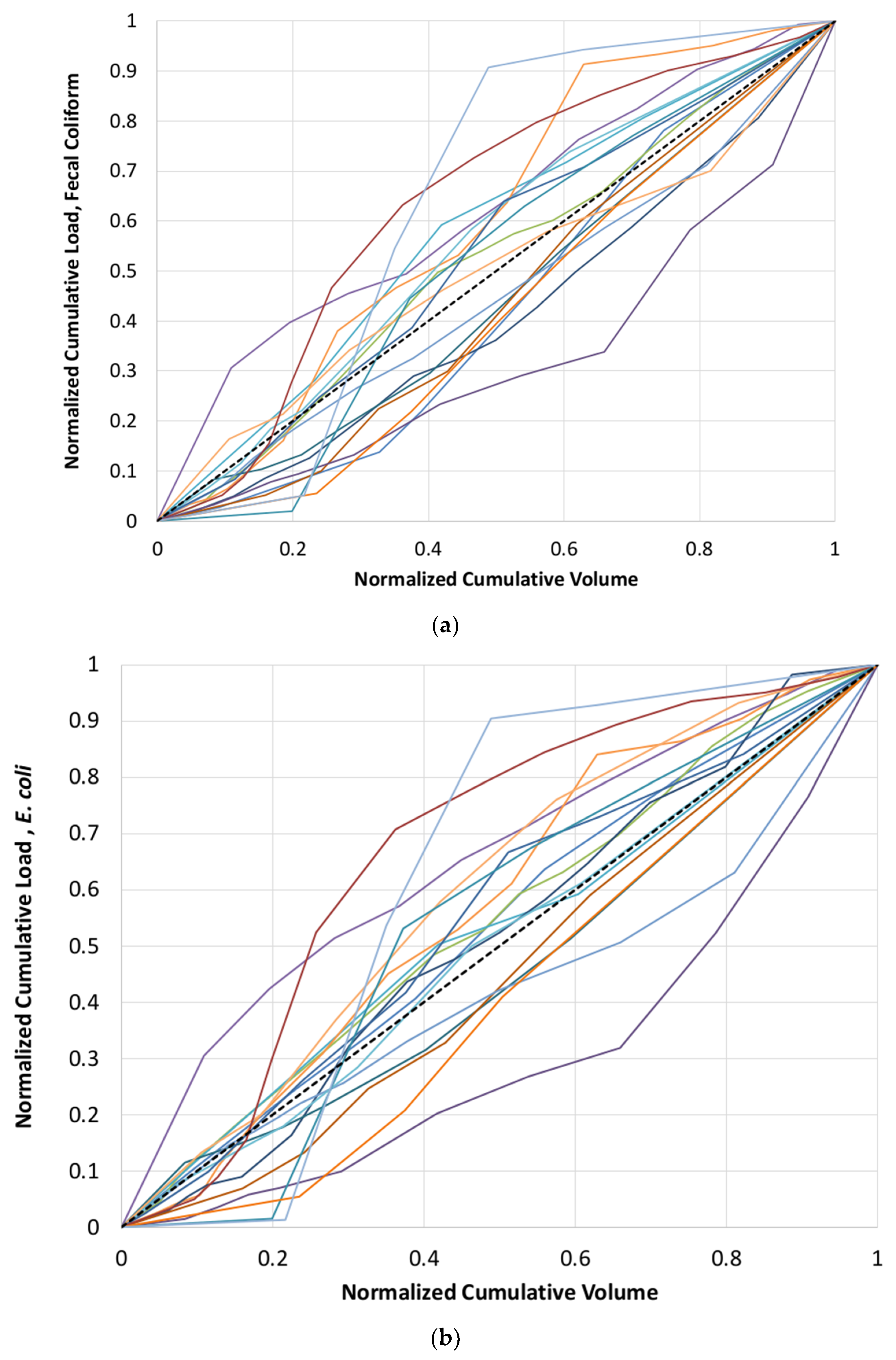
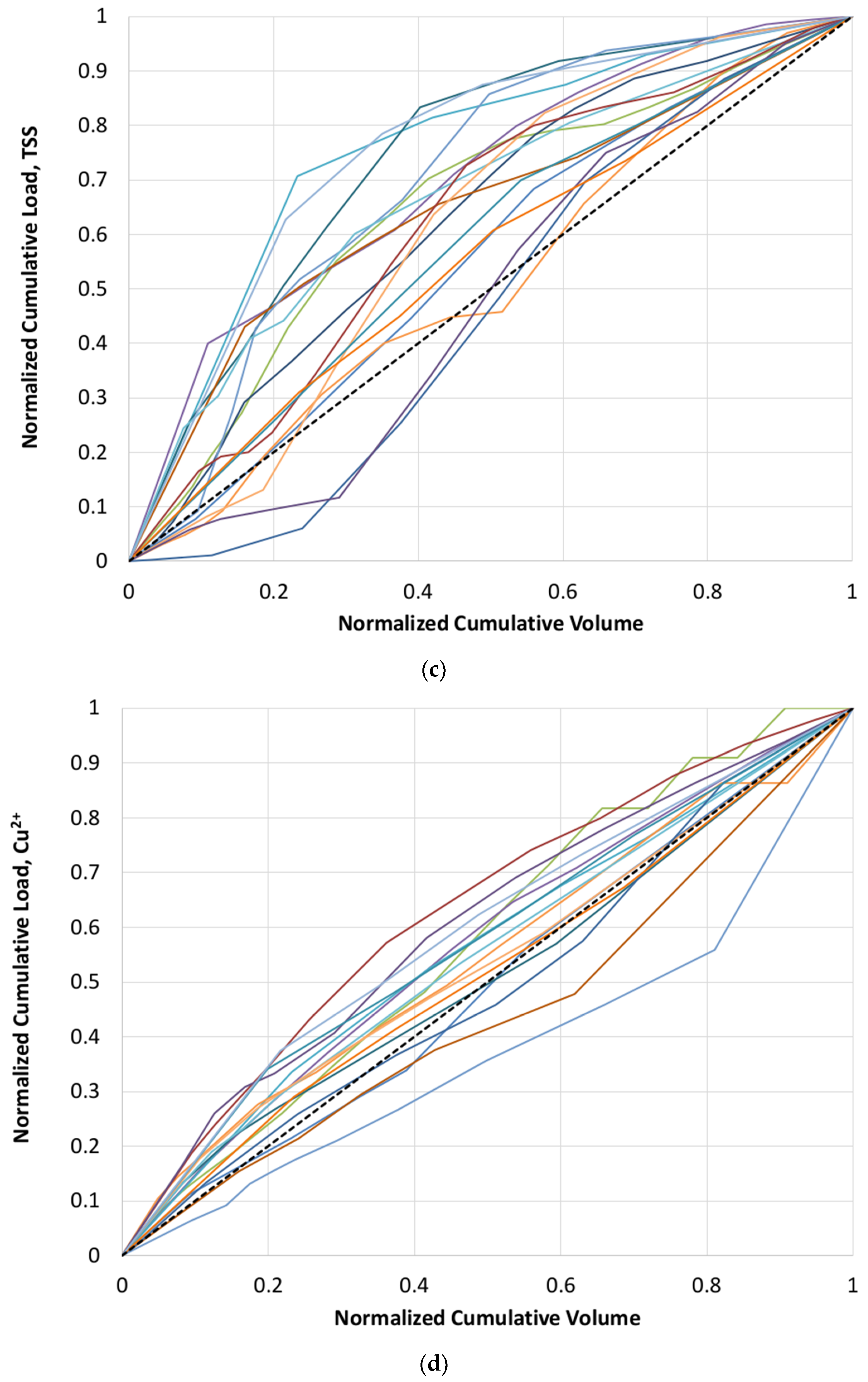
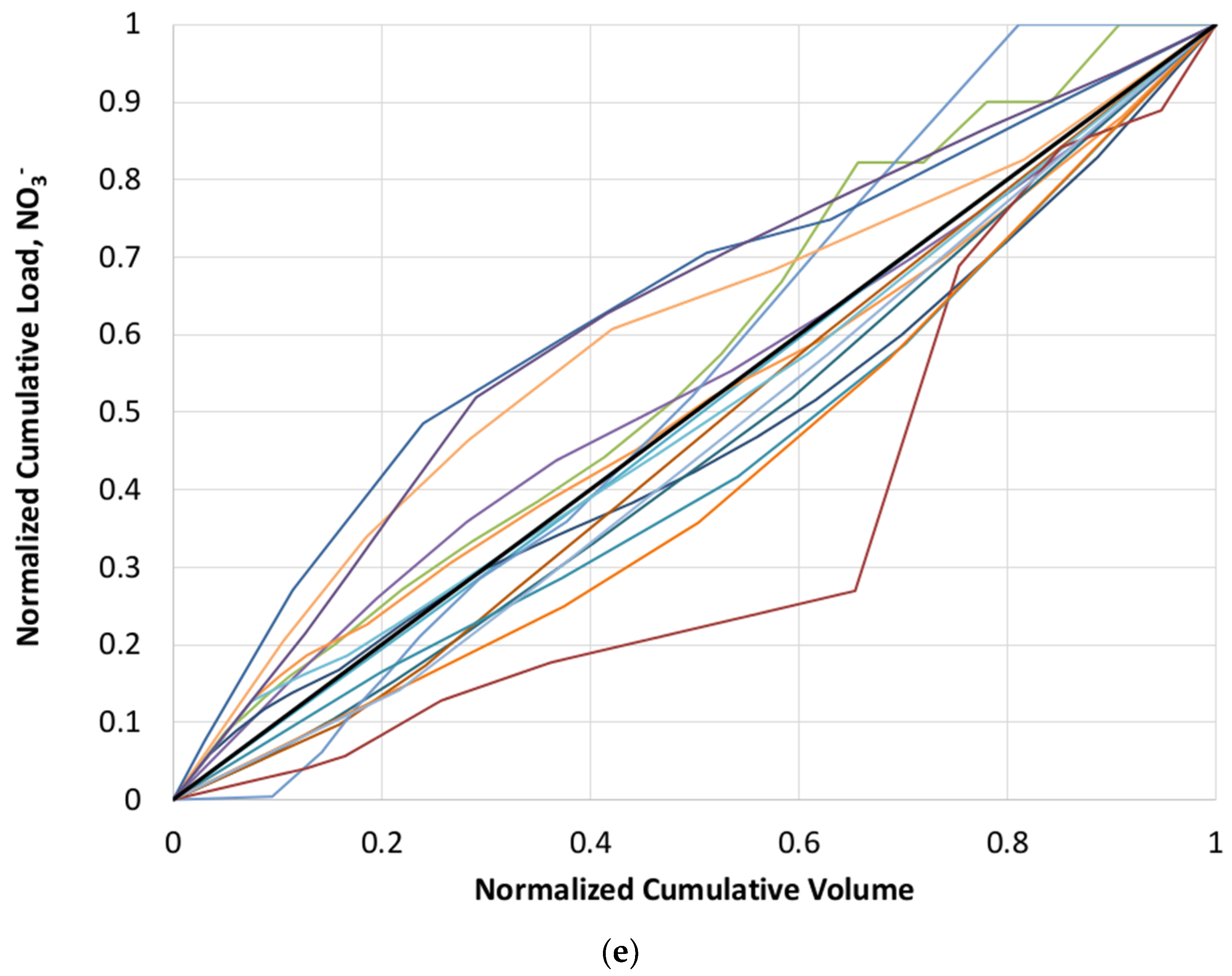
2.4.1. FF₃₀: Traditional First Flush Analysis

As noted above, borrowing from urban stormwater literature to quantify the presence and strength of the first flush allows an initial understanding of pollutant temporal distributions in the stream flow. Although uncommon for use in stream science, this methodology allows direct comparison of results to previous studies performed on smaller urban upland catchments. The normalized cumulative runoff volume (V’) versus cumulative pollutant mass (M’) was calculated for each storm event and watershed (Equations (1) and (2)). The strength of the first flush was defined as the percentage of total pollutant load delivered in the first 30% of event volume, or FF₃₀ (i.e., a threshold methodology—see Equation (3)). While a variety of different thresholds have been used in literature, this is consistent with many recent studies, allowing comparison of results [12,19,29].

$$F{F}_{30}= {\displaystyle \sum }_{V=0}^{V=30\%\left(Vtot\right)}{P}_v$$

(3)

where V is stormwater volume (m³) defined at a particular point during the storm, V_tot is the total volume of runoff during an event (m³), and P is pollutant load.

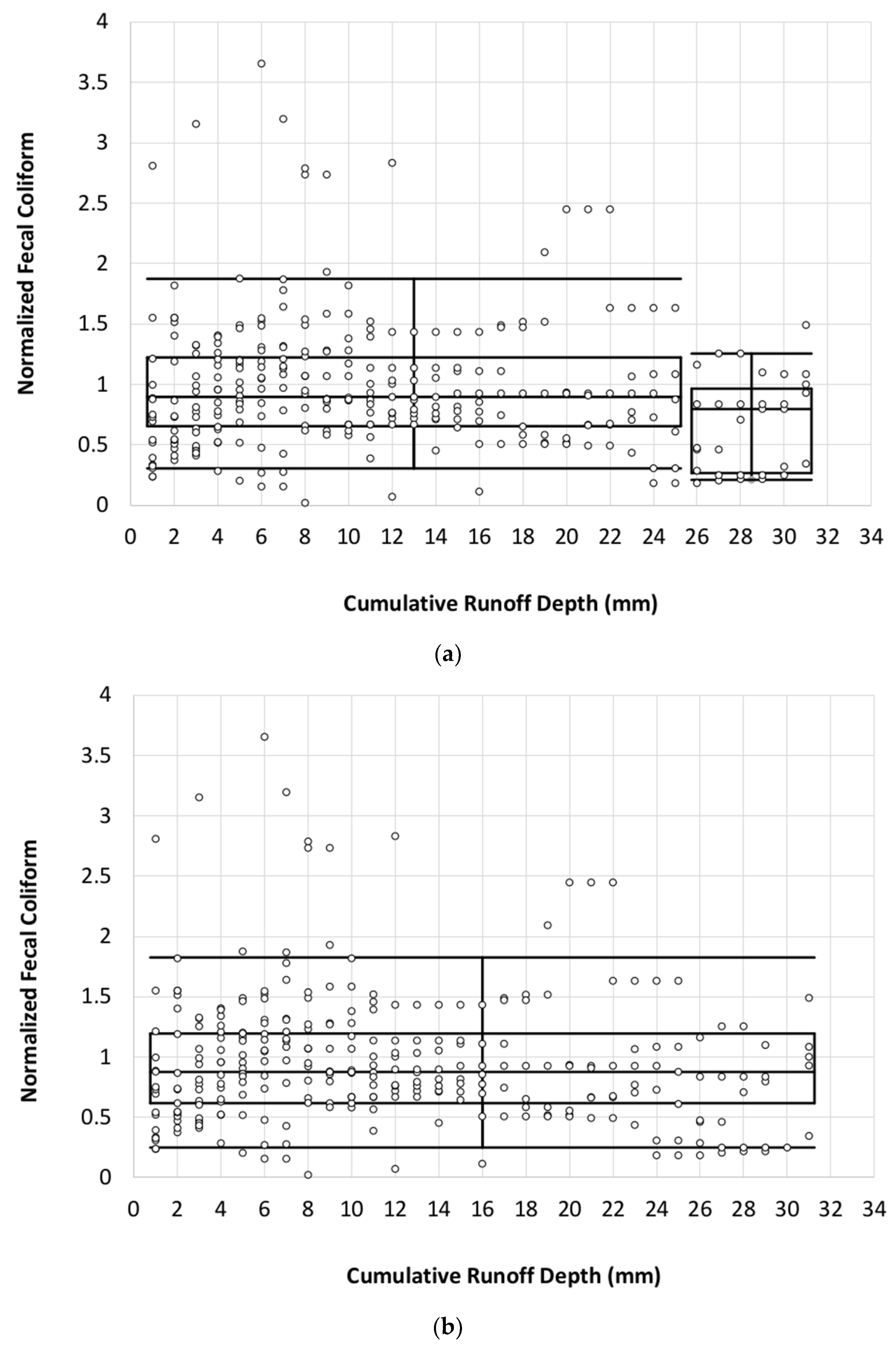
2.4.2. Bach Slice Method

A different definition used to quantify the first flush was introduced by Bach et al., 2010 [19]. To perform this assessment, each storm event was parsed into slices of runoff depth per the methods of Bach et al., 2010 [19]. For each slice, the pollutant concentrations are interpolated for each event to represent the slice’s average pollutant concentration (Equation (4)). The pollutant concentrations were normalized by dividing by the event mean concentration to make concentrations associated with different events comparable, that is, to reduce the effect of inter-event variability. Adjacent grouping of slices based on the Wilcoxon rank sum test and a 5% level of statistical significance occurs until the next slice of statistical difference is found; then a new group is started. If all the slices from one site location can be grouped into one large slice, and thus all slices are statistically similar, then the first flush did not occur. The first flush did occur if there is more than one slice group. For more details on this methodology see Bach et al., 2010 [19].

$${\overline{C}}_{slice}=\frac{{{\displaystyle \sum }}_{slice begin}^{slice end}{C}_i{Q}_i∆t}{{{\displaystyle \sum }}_{slice begin}^{slice end}{Q}_i∆t}$$

(4)

where $\overline{C}$ is the average concentration for a given slice, C_i is the concentration at a given point in time, Q_i is the flow rate at a given point in time, and ∆t is the time between measurements.

2.4.3. Antecedent Climate and Other Explanatory Variables

Two tipping bucket rain gauges were installed and used for the Second Creek site, one approximately at the midpoint of the watershed, and one at the outlet. Rainfall data were collected at 1 min increments. When both measurements were available, the Thiessen polygon method was used to provide a weighted average of rainfall. However, the gage located near the watershed outlet was typically in operation more frequently and was used singularly when necessary. Temperature and relative humidity data from nearby Knoxville Tyson-McGee Airport were obtained using the NC CRONOS database (version 2.7.2, State Climate Office of North Carolina, Raleigh, NC, USA). The explanatory variables were chosen based upon previous work by Hathaway and Hunt, 2010 [30], McCarthy, 2009 [31], and McCarthy et al., 2012 [32]. Antecedent climate was characterized for the 2 days and 28 days preceding the event. These values were chosen based on the work of Hathaway et al., 2010 [29], who found that these periods of time allowed an understanding of the influence of more recent climate characteristics (2 days) vs. those that have been consistently occurring for a longer period of time (28 days). The antecedent dry weather period (ADWP) variable was determined by calculating the number of days since 1.3, 2.5, or 12.7 mm of rainfall occurred.

2.5. Statistical Analysis

Due to the small sample size and consistently non-normal distributions of the data, non-parametric tests were utilized and performed using JMP Pro Version 12 (SAS Institute, Cary, NC, USA). The Wilcoxon rank sum test was used to determine statistical difference between slices (as discussed previously) and to determine the statistical significance of FF₃₀. The Spearman rank test was performed on each pollutant for Second Creek using various explanatory variables and FF₃₀ values. In the case that any climate data were missing for a given event, the test was conducted with a smaller sample size as needed. There are not enough events for the sample results to be confident for Third Creek.

3. Results and Discussion

Between September 2014 and August 2016, a combined 24 total storm events were collected and tested for pollutants from both creeks. Each storm was represented by at least five discrete samples, with the maximum number of representative samples being 18 and the average being nine. As described above, analyses included fecal coliform, E. coli, TSS, Cu²⁺, and NO₃⁻ (Table 1). However, two events from Second Creek are missing Cu²⁺ and NO₃⁻ data, and one event from Third Creek is missing TSS data.

3.1. FF₃₀: Traditional First Flush Analysis

3.1.1. Overall Observations and Trends

The range of observed FF₃₀ varied by pollutant type at each site and no pollutant exhibited a first flush for all events (

Table 2. Summary statistics of FF₃₀: maximum, minimum, mean, median, and RSD for fecal coliform, E. coli, TSS, Cu²⁺, and NO₃⁻.

Site	Pollutant	Fecal Coliform	E. coli	TSS	Cu2+	NO3−
Second Creek	% storms with FF30 > 0.3	53	65	88	81	44
	Max	0.53	0.6	0.75	0.49	0.53
	Min	0.12	0.11	0.13	0.21	0.15
	Mean	0.3	0.32	0.47	0.36	0.32
	Median *	0.31	0.32	0.46	0.37	0.3
	RSD (%)	40	38	38	20	36
Third Creek	% storms with FF30 > 0.3	71	71	83	86	43
	Max	0.87	0.88	0.55	0.46	0.39
	Min	0.14	0.25	0.29	0.27	0.25
	Mean	0.51	0.42	0.39	0.34	0.3
	Median	0.49	0.35	0.39	0.32	0.29
	RSD (%)	60	60	26	19	16

* Medians tested for statistical difference from 0.3, p-value < 0.05 in bold, p-value < 0.1 underlined.

). In most literature, first flush strength has typically increased with decreasing catchment size [13,14,33]. However, in this study, both watersheds showed fairly similar first flush strength and variability. It should be noted that in comparison to past study sites, even the smallest watershed (Second) is still fairly large at 1800 ha. Thus, the effect of catchment size may be more pronounced along the gradient of watershed areas smaller than those studied here. See Figure 2 for example Second Creek pollutagraphs where each line represents the M’-V’ line for an individual event.

The first flush strength (median FF₃₀) for the constituents at Second Creek and Third Creek, respectively, are as follows: TSS > Cu²⁺ > E. coli > fecal coliform > NO₃⁻, and fecal coliform > TSS > E. coli > Cu²⁺ > NO₃⁻. Even though FF₃₀ was high for some pollutants, like Third Creek’s fecal coliform (Table 2), no statistically significant differences between pollutants were found (p < 0.05). This is most likely due to small sample numbers or high variability in the data as evidenced by the relative standard deviation (RSD) of the pollutant.

3.1.2. Total Suspended Solids

TSS had the highest median FF₃₀ (Table 2) for Second Creek, and FF₃₀ was significantly higher than 0.3 for both watersheds (p < 0.05). Median FF₃₀ was found to be 0.46 and 0.39, at Second and Third Creeks, respectively. Past literature from urban upland catchments supports these findings, with some degree of sediment first flush generally being present and seemingly more perceptible than for other pollutants [16]. As an example, studies such as Hathaway and Hunt, 2011 [29] found a relatively high median TSS compared to other literature with an FF₃₀ of 0.47, while Taebi and Droste, 2004 [16], found 30.9% of TSS load and Deletic, 1998 [2], found 25.5% and 31% of the TSS load (for two watersheds) to be delivered in the first 20% of event volume on average. Overall, multiple studies concluded some sort of flush occurred for TSS [2,12,15,19,34]. While past studies have found TSS to have consistent first flushes, they are often weaker than the FF₃₀ values found in this study. This may be due to the site locations, where open channel streams are able to contribute resuspended sediment to the flow during storm events. Since this study was performed in one specific physiographic region, results may vary for streams with different substrate and/or different levels of channel stability from the streams studied herein.

3.1.3. Microbes

Fecal coliform and E. coli were more variable than other pollutants as seen by their relatively larger RSD, with Third Creek microbe FF₃₀ values being higher than those of Second Creek. Indicator bacteria have been found to have high variability in literature. Past studies on urban upland catchments have not found E. coli to have a consistent first flush with median FF₃₀ being 0.27, 0.28, 0.29, 0.33, and 0.40 in five watersheds from two notable studies [29,31]. For Second and Third Creeks, median FF₃₀ was at the upper range of that reported in literature being 0.32 and 0.35, respectively. A similar trend was observed when the percentage of storm events with an FF₃₀ greater than 0.3 (i.e., those that show a first flush) was analyzed. For the five watersheds evaluated by Hathaway and Hunt, 2011 [29], and McCarthy, 2009 [31], 44%, 44%, 45%, 56%, and 65% of events showed a first flush. In this study, more consistency was noted in the first flush effect, with 65%, and 71% of storms exhibiting a first flush for Second and Third Creeks, respectively. Streambeds are stores for microbes as past literature has explained [7,35,36], potentially leading to their resuspension during storm events when the bed is mobilized. This may explain E. coli’s first flush significance at Second Creek, and E. coli’s first flush event frequency at Third Creek.

3.1.4. Copper and Nitrate

The lowest average RSD (least variable FF₃₀) was observed for Cu²⁺ and NO₃⁻. Dissolved constituents, like Cu²⁺ and NO₃⁻, typically do not show a consistent or strong first flush in literature and this is the same conclusion for NO₃⁻ herein [4,13,37]. However, Cu²⁺ is the second strongest constituent at Second Creek and the strongest at Third Creek. A study by Sansalone and Buchberger, 1997 [3], found a pronounced first flush for dissolved Cu from an urban roadway for lateral pavement sheet flow; although, it should be noted that this was determined by using a first flush definition of m(t) > v(t). Using the first flush definition of 50% pollutant delivered in the first 25% volume, a study by Flint and Davis, 2007 [34], on an urban upland catchment found only 21% events for Cu²⁺ and 22% events for NO₃⁻ had a first flush from an entirely impervious roadway. First flush presence of Cu²⁺ is more frequently identified in this study, however, it is lower in strength than the TSS first flush frequency. The differences in the strength of various pollutants between watersheds suggests that site specific variables influence pollutant transport trends such as the geospatial arrangement of impervious surfaces.

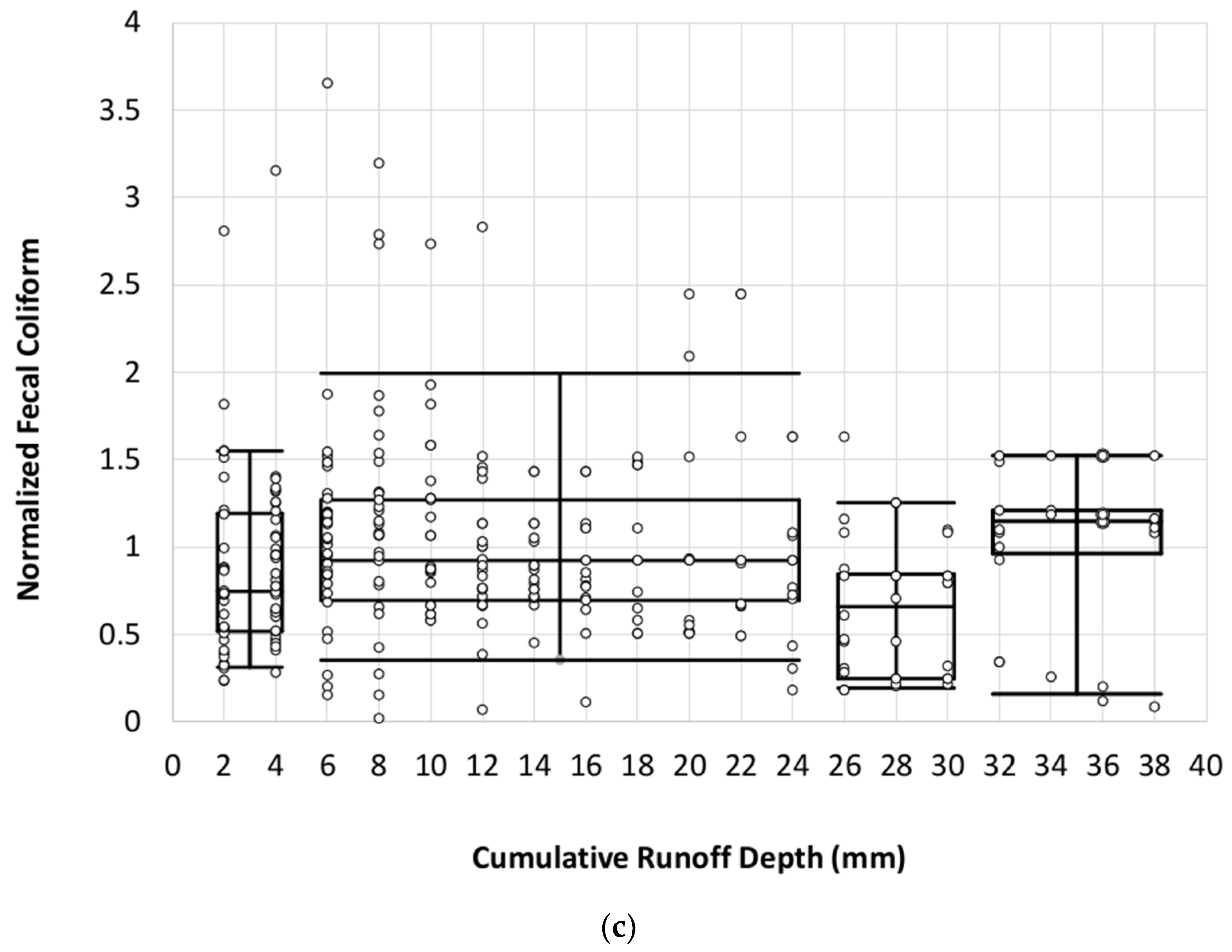
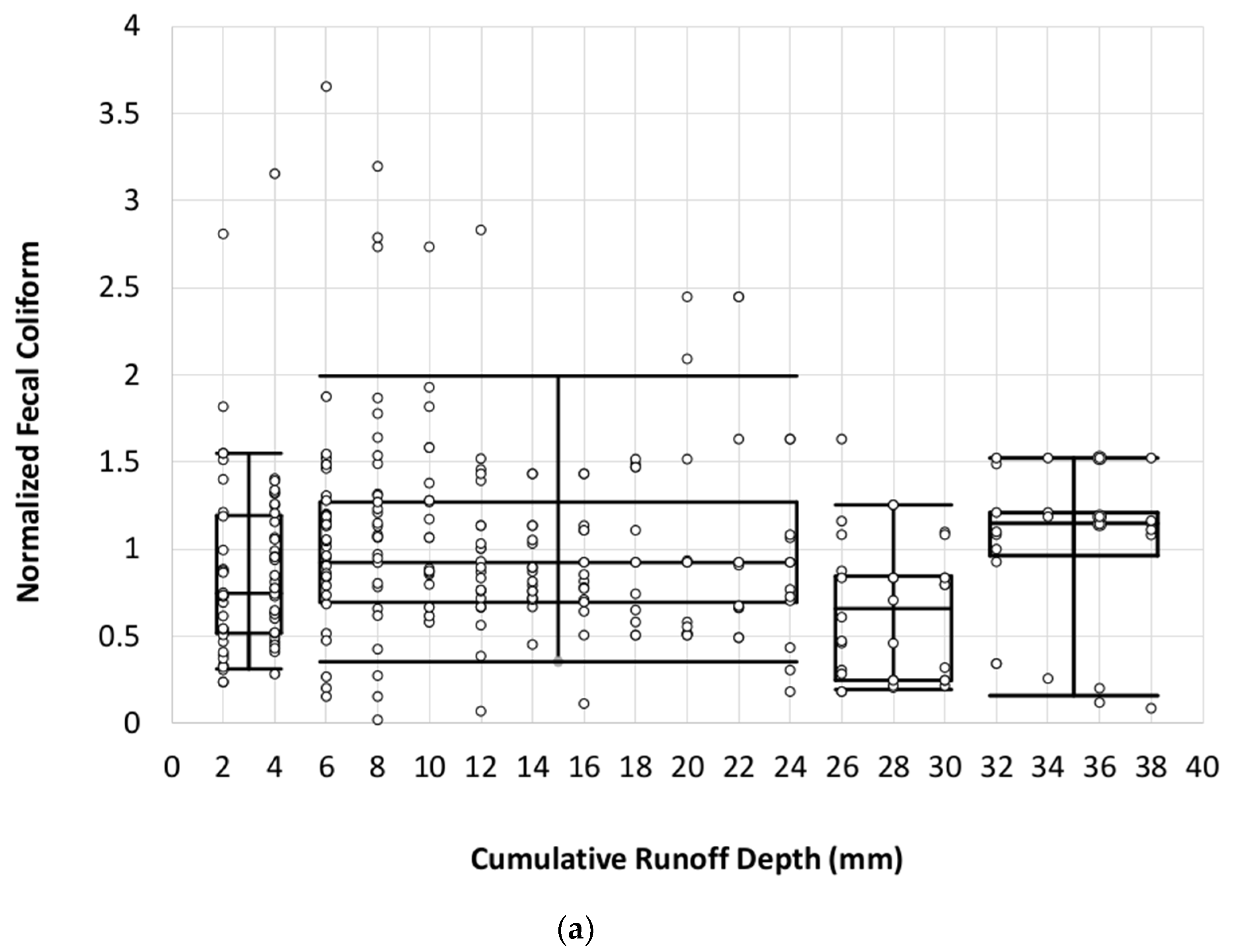
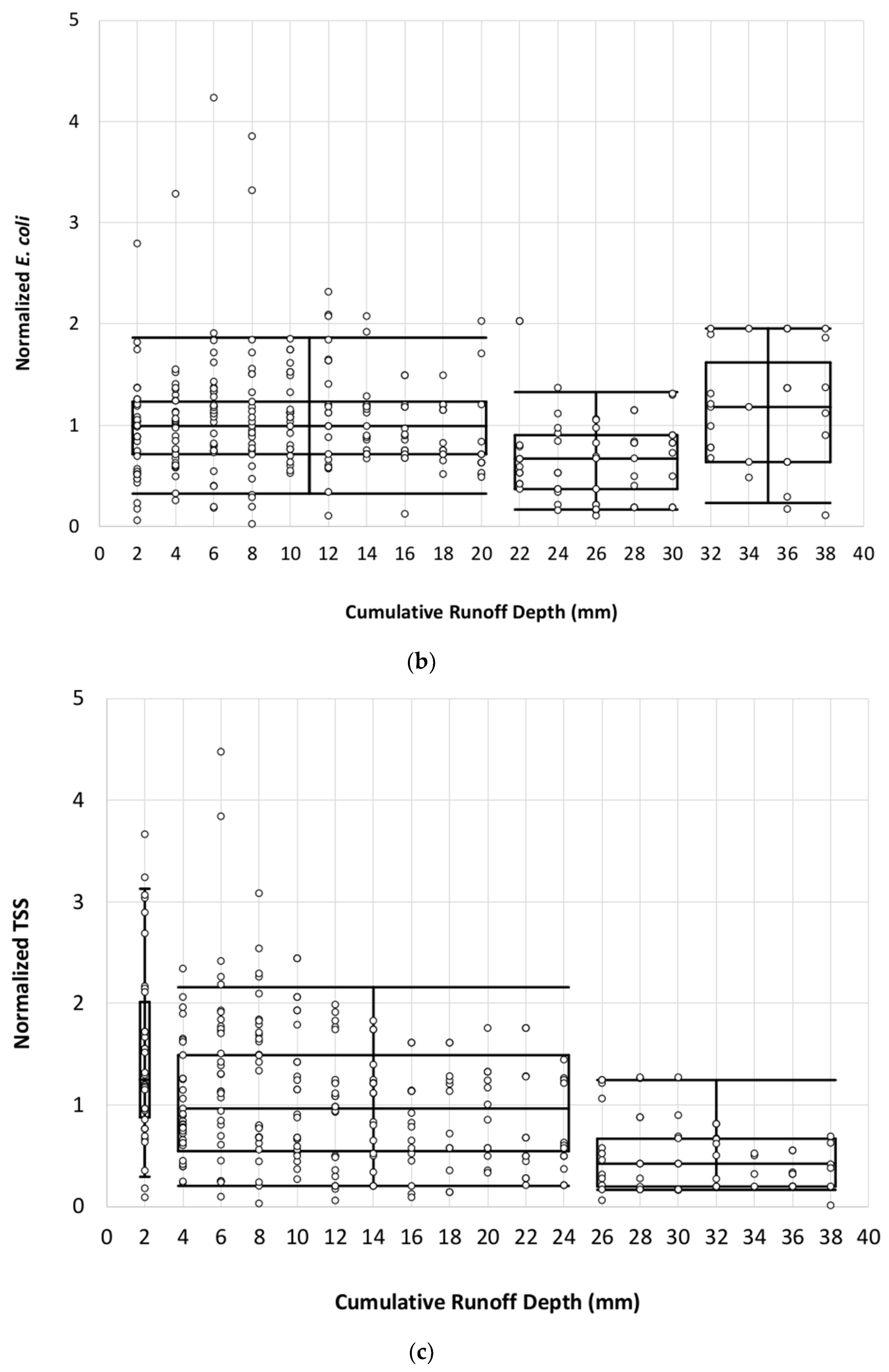
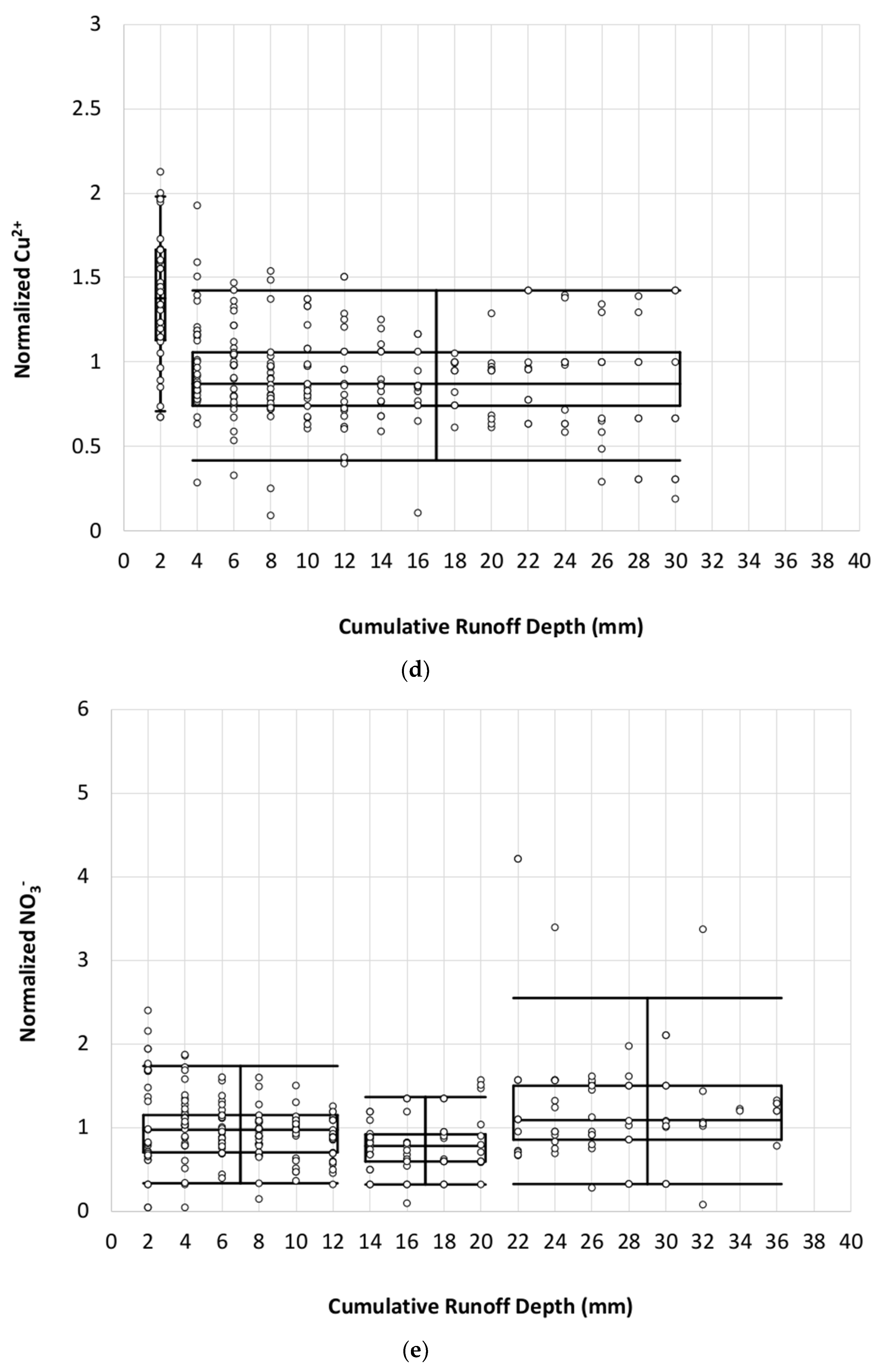
3.2. Bach Slice Method

Figure 3 and Figure 4 illustrate the Bach method results. For these figures, the Y-axis represents the normalized pollutant concentration, which is the concentration for each sample collected normalized by the average concentration during the event in which it was collected (to minimize the effect of inter-event variability on the analysis as noted above). On the X-axis, runoff depths are shown with the maximum being the largest depth represented by at least three data points. Individual circles are normalized concentrations for each sample collected during the study. After statistical analysis provided an understanding of which slices were statistically similar, and could thus be grouped, boxplots were created for each statistically similar group of slices using the individual normalized concentrations in each group.

Slice size selection was directed by two factors: (1) Bach et al., 2010 [19], stated slice size sensitivity was not significant when comparing sizes between 0.5 and 3 mm; (2) they suggested the slice size should be chosen as the smallest slice that has at least one explicitly measured data point rather than all data within that slice containing interpolated data. A slice size of 1 mm met that criteria; however, the results of the Wilcoxon rank sum test used to evaluate significant differences in slices showed only significant differences in the latter part of the cumulative runoff depth. For example, a new slice group started after an initial slice size of 28 mm for Second Creek’s TSS. This outcome was not consistent with other studies that have noted a first flush effect for TSS, and the traditional first flush analysis implied a strong flushing effect prompting further analysis. To verify the slice size sensitivity for these data, calculations were rerun with a 2 mm slice size. Results showed contaminants that typically have a first flush (i.e., TSS) still were not being represented as such. Next, instead of using average concentrations within the 2 mm slice size for each event, data were combined by considering the concentrations of 1 and 2 mm (without averaging) and renaming as 1–2, 3 and 4 mm renamed 3–4 and so on, effectively doubling the sample size. This method seemed to more accurately represent the data and various pollutants’ first flush. This is likely due to increased statistical power gained with a larger number of data points in each slice (Figure 3).

Second Creek had the highest maximum runoff depth due to a number of larger events being monitored relative to the other site. A first flush occurred when two or more box and whisker plots, or groups, were present. The only pollutants that did not have more than one group are E. coli and NO₃⁻ from Third Creek. Additionally, of note were Second Creek’s fecal coliform (Figure 4a), E. coli (Figure 4b), and NO₃⁻ (Figure 4e); and Third Creek’s Cu²⁺ boxplots where inconsistent trends were observed, that is, both increases and decreases were noted in groups as runoff depth increased. The other two studies that used this method did not observe such trends but also did not have more than three slices or utilize the same procedure for grouping slices.

Using the Bach method, the first flush strength and first flush depth can be quantified. The strength of the first flush, or P_FF, is defined as the p-value of the Wilcoxon rank sum analysis between the first and last group (

Table 3. Summary of analysis methods.

Site	Parameter	P30%	PFF	Median FF30	Initial Group Size (mm)	VFF (mm)	Boxplot Trend
Second Creek	Fecal Coliform	0.554	0.0846 **	0.31	4	30	Inconsistent
	E. coli	0.0704	0.3159	0.32	20	30	Inconsistent
	TSS	<0.0001	<0.0001	0.46	2	24	First flush
	Cu2+	0.0006	<0.0001	0.37	2	2	First flush
	NO3−	0.5192	0.2908	0.3	12	20	Inconsistent
Third Creek	Fecal Coliform	0.1724	<0.0001	0.46	2	2	First flush
	E. coli	0.1724	0.1350 *	0.33	28	2*	No first flush
	TSS	0.0493	0.0016	0.39	2	2	First flush
	Cu2+	0.0204	<0.0001	0.32	6	14	Inconsistent
	NO3−	0.6832	0.2124 *	0.29	28	8*	No first flush

* Results did not exhibit first flush (1 box), lowest p-value between slices reported. ** Last slice significantly higher than first. p-value < 0.05 in bold p-value < 0.1 in underline.

). The Bach method also determines first flush volume, V_FF, to be the runoff depth up to the beginning of the last slice. If a pollutant has a high V_FF, this indicates the high concentration in the first flush takes a significant amount of runoff to be reduced.

Half of the contaminants exhibited a first flush, as defined by a P_FF < 0.1, including: Second Creek’s TSS and Cu²⁺; and Third Creek’s fecal coliform, TSS, Cu²⁺. TSS and Cu²⁺ are the only pollutants to show a first flush at both sites when p < 0.05. It should also be noted that some pollutants exhibited an “inconsistent” first flush (further described above). For example, fecal coliform for Second Creek actually exhibited significantly higher concentrations in the last slice of runoff (p < 0.1). Similar, but statistically insignificant, trends were noted for E. coli and NO₃⁻ at Second Creek. This may suggest the influence of pollutant and runoff origin, whereby the initial runoff from highly connected impervious surfaces may contain lower concentrations of bacteria and nutrients compared to runoff from other surfaces (see Epps and Hathaway, 2018 [38]) and/or wastewater intrusion that may contribute to in-stream flows with higher runoff depths. Conversely, pollutants such as sediment and metals may have comparably higher buildup on these connected impervious surfaces and show a stronger first flush.

For those pollutants that did not exhibit a first flush or for which the first flush was only noted for one group, the lowest p-value and the runoff depth at which a first flush is likely to occur is reported. From Table 3, Second Creek’s fecal coliform, E. coli and NO₃⁻ do not have a statistically significant (p < 0.05) first flush between the first and last slices and also exhibited one of the inconsistent trends. This is most likely due to the observed end flush occurring on the last slice for both these contaminates. This is not the first time an end flush has been seen in literature, particularly for indicator bacteria. Other studies for upland catchments suggested end flushes could be due to wastewater intrusions or land use characteristics [29,31]. For NO₃⁻, a small number of baseflow samples from Second Creek suggested higher concentrations may be present in baseflow than during a runoff event. Thus, it is possible that as baseflow became a larger component of the overall flow at the end of the event, NO₃⁻ concentrations were elevated, resulting in the observed pattern.

3.3. Synthesis of Method Outcomes

Results from the traditional method and the Bach method were synthesized to understand how they compared. When looking at median FF₃₀ from the traditional method, all of the pollutants with inconsistent trends or one group (per the Bach first flush method) have a median between 0.29 and 0.33. Whereas, Second Creek’s TSS and Cu²⁺, and Third Creek’s fecal coliform and TSS have FF₃₀ medians between 0.37 and 0.46, which is typically corroborated by a first flush in the boxplot graph generated as part of the Bach et al., 2010 [19], method. This relationship suggests FF₃₀ medians are typically higher for those boxplot graphs expressing a consistent first flush per the Bach method, with a consistent downward trend in concentration as runoff depth increases.

Qualitative observation of the Bach method graphs (Figure 4) also corroborated the first flush strength when compared to the FF₃₀. These first flush pollutant plots have an initial grouping which constitutes 2–4 mm of runoff depth followed by other groups with decreasing values. The smaller the runoff volume represented by the first group, and the higher the magnitude of this group in comparison to subsequent groups, the higher the FF₃₀ median.

Although the traditional first flush method is the most commonly implemented in literature, results from the Bach method appear comparable and provide additional information regarding pollutant transport. As noted above, the selection of the slice depth does appear to pose a source of error in the analysis. Various slice depths and combinations of slice depths created variable results. This represents a need for future study. Despite this potential uncertainty due to slice size selection, substantially more information is gained through the Bach method. The identification of “inconsistent” and “end flush” trends in the data are more easily identified in the Bach method, leading to valuable insights on pollutant transport. Further, the Bach method allows observation of the influence of runoff depth on transport trends. For urban systems where runoff generation is highly variable based on watershed impervious connectivity, this is valuable insight.

3.4. Influence of Antecedent Climate and Event Specific Parameters

To better understand the causes of the variable FF₃₀ values between storms, the Spearman rank test (

Table 4. Spearman rank correlation analysis between flow, rainfall, and antecedent climate explanatory variables and pollutants.

		Fecal Coliform		E. coli		TSS		Cu2+		NO3−
		rs	p-Value	rs	p-Value*	rs	p-Value	rs	p-Value	rs	p-Value
Antecedent Climate	Max. Temp28 days	−0.46	0.0631	−0.54	0.0249					−0.50	0.0456
	Max. Temp2 days	−0.45	0.0730	−0.58	0.0140					−0.47	0.0645
	Min. Temp28 days	−0.46	0.0631	−0.54	0.0249					−0.50	0.0456
	Min. Temp2 days	−0.44	0.0759	−0.59	0.0313					−0.48	0.0570
	Min. RH28 days							−0.48	0.0598	0.54	0.0310
	Total Rainfall28 days					0.87	0.0003
	ADWD0.1			0.46	0.0745
Rainfall	Total Rainfall							−0.60	0.0297	0.49	0.0869
	Ave. Rainfall Intensity							−0.50	0.0824	−0.70	0.0073
	Max. Rainfall Intensity	−0.46	0.0996					−0.71	0.0066	−0.54	0.0577
Storm-water flow	Max. Flow Rate	−0.62	0.0075	−0.46	0.0608			−0.61	0.0113
	Ave. Flow Rate	−0.51	0.0374					−0.60	0.0132

*: p-value < 0.05 in bold.

) was performed on each pollutant for Second Creek comparing various explanatory variables and FF₃₀ values. There were not enough events for the sample results to be valid for Third Creek, thus it is not discussed further. The results of this assessment are described below.

3.4.1. Antecedent Climate

Antecedent temperature was found to negatively correlate to the FF₃₀ of fecal coliform, E. coli, and NO₃⁻. Similarly, Hathaway and Hunt, 2011 [29], found fecal coliform FF₃₀ was negatively correlated to antecedent temperature in an urban upland catchment (i.e., the first flush was weaker as temperatures increased); however, no correlation was found between temperature and E. coli FF₃₀. The study hypothesized that the first flush of microbes during the warmer summer months was weak because there are higher concentrations of microbes blanketing the watershed versus in the winter months when the microbes are more source limited. E. coli FF₃₀ is the only constituent to correlate to ADWP (antecedent dry weather period). As ADWP decreased, the FF₃₀ decreased. This trend is likely explained by flushing within the system, that is, if frequent rainfall has been occurring, the microbial store is depleted resulting in more consistent concentrations.

The explanation for the negative correlation between temperature and the NO₃⁻ FF₃₀ is uncertain. This suggests that as temperatures increase, a weaker first flush is observed. This could be due to the ubiquity of fertilizers during the summer months making this pollutant rarely if ever source limited. Studies such as Toran and Grandstaff, 2007 [39], stress the effect of a lack of data regarding homeowners use and timing of fertilizer, and suggest the importance of these variables on nutrient variability. It is also possible that seasonal variations in biological processes such as organic matter decomposition exist within the watersheds.

The antecedent total rainfall was positively and strongly correlated to the FF₃₀ of TSS. There were no other variables that correlated to TSS FF₃₀ despite some previous literature for upland catchments which showed the TSS first flush related to other rainfall related parameters such as rainfall depth, peak rainfall intensity, storm duration, antecedent dry weather period [2,13,16,40]. It is possible that in Second Creek, there is an initial response for sediment no matter climate, rainfall, or flow factors, which would be more consistent with in-stream processes as opposed to those in the upland.

3.4.2. Rainfall

Three rainfall variables, total rainfall, average rainfall intensity, and max rainfall intensity, correlated to the FF₃₀ of the dissolved pollutants, Cu²⁺ and NO₃⁻. Correlations were negative other than for NO₃⁻ FF₃₀ and total rainfall, indicating that larger and/or more intense storms have a weaker first flush. For smaller events, most of the runoff is likely delivered from connected impervious surfaces such as roadways, where a first flush for Cu²⁺ has been shown to be more frequent [3]. Larger, more intense storm events have pervious and disconnected areas contributing, potentially making Cu²⁺ concentrations more consistent with the addition of other sources of pollution. This explanation is speculative and is an area for further research.

3.4.3. Stormwater Flow

Microbes were negatively correlated to flow rate, so with high flow rates a weak first flush was exhibited. Surbeck, Jiang, Ahn, and Grant, 2006 [41], found microbes to increase abruptly and remain elevated after flow increased in-stream from three storm events monitored at three different locations in southern California. Therefore, higher flows could result in elevated levels of microbes that stay suspended over an event, resulting in a weak first flush. A stronger first flush for microbes may have occurred at lower flow rates because fewer microbes were mobilized, or those that were mobilized settled more quickly.

4. Conclusions

This study revealed notable relationships for in-stream temporal pollutant variability, in particular in comparison to past studies on upland urban watersheds. When compared to past research which utilized the traditional first flush method and is typically conducted in urban upland catchments, this study seems to have more consistent and substantial first flush effects for pollutants such as TSS and microbes. Notable outcomes also came from an assessment comparing traditional first flush analyses to a newer method. Using this newer method, Bach et al., 2010 [19], identified more pollutants that exhibited a first flush than the traditional method results. However, after comparing the two methods in this study, it appeared the FF₃₀ median from the traditional method supported conclusions from the Bach method.

This study brings insight as to how in-stream processes may affect pollutant load. Past studies have shown the first flush for sediment and microbes do occur in-stream from increased flows [7,35]. This study found a significant first flush occurred for TSS in-stream at all site locations. Further, despite not identifying a consistent statistically significant first flush for microbes (based on FF₃₀), a relatively high percent of storms showed a first flush for fecal coliform at both Second Creek and Third Creek based on this metric (65% and 71% of storms, respectively).

Inconsistent trends were observed for microbes based on the Bach method. While Third Creek showed a significant first flush for fecal coliform based on P_FF, an end flush of microbes and NO₃⁻ was observed for Second Creek. The ability to identify and quantify this end flush using the Bach method was noted to be a particular strength of this approach and indicates the potential presence of other sources of microbes during large events (such as from wastewater and/or loss from more permeable sources). Thus, although the results from the two first flush methods typically agreed, some small differences in the approaches and the information gained were seen for microbes.

From the correlation analysis between the strength of the first flush (FF₃₀) and possible explanatory variables for changes in FF₃₀, a few interesting trends developed. First, microbial FF₃₀ was again correlated to temperature as has been shown in other studies by Hathaway and Hunt, 2011 [29]; however, the addition of flow as a correlating factor was new. The strong influence of rainfall and flow variables on Cu²⁺ were also notable in light of the strong first flush shown for this parameter. As rainfall depth and/or flow rates increased, the strength of the first flush decreased. This may be due to the preponderance of runoff that occurs from roadways in comparison to other land uses during small events.

Further studies, especially in-stream, looking into the relationships between water quality parameters and their explanatory variables could enhance our understanding of pollutant export in urban watersheds. Results from this study suggest that in-stream temporal changes can be substantial for pollutants such as TSS. Therefore, there may be a need to incorporate an in-stream pollutant model into current water quality models for urban watersheds.

References

1. Makepeace, D.K.; Smith, D.W.; Stanley, S.J. Urban stormwater quality: Summary of contaminant data. Crit. Rev. Environ. Sci. Technol. 1995, 25, 93–139. [Google Scholar] [CrossRef]
2. Deletic, A. The first flush load of urban surface runoff. Water Res. 1998, 32, 2462–2470. [Google Scholar] [CrossRef]
3. Sansalone, J.J.; Buchberger, S.G. Partitioning and First Flush of Metals in Urban Roadway Storm Water. J. Environ. Eng. 1997, 123, 134–143. [Google Scholar] [CrossRef]
4. Characklis, G.W.; Wiesner, M.R. Particles, Metals, and Water Quality in Runoff from Large Urban Watershed. J. Environ. Eng. 1997, 123, 753–759. [Google Scholar] [CrossRef]
5. Peter, K.T.; Hou, F.; Tian, Z.; Wu, C.; Goehring, M.; Liu, F.; Kolodziej, E.P. More Than a First Flush: Urban Creek Storm Hydrographs Demonstrate Broad Contaminant Pollutographs. Environ. Sci. Technol. 2020, 54, 6152–6165. [Google Scholar] [CrossRef]
6. Pachepsky, Y.; Guber, A.; Shelton, D.; Hill, R. E-coli resuspension during an artificial high-flow event in a small first-order creek. In Proceedings of the EGU General Assembly Conference Abstracts, Vienna, Austria, 19–24 April 2009. [Google Scholar]
7. Surbeck, C.; Shields, F.D.; Cooper, A.M. Fecal Indicator Bacteria Entrainment from Streambed to Water Column: Transport by Unsteady Flow over a Sand Bed. J. Environ. Qual. 2016, 45, 1046–1053. [Google Scholar] [CrossRef]
8. Ferguson, C.; Husman, A.M.D.R.; Altavilla, N.; Deere, D.; Ashbolt, N.J. Fate and Transport of Surface Water Pathogens in Watersheds. Crit. Rev. Environ. Sci. Technol. 2003, 33, 299–361. [Google Scholar] [CrossRef]
9. Helsel, D.; Kim, J.; Grizzard, T.; Randall, C.; Hoehn, R. Land use influences on metals in storm drainage. J. Water Pollut. Control Fed. 1979, 51, 709–717. [Google Scholar]
10. Saget, A.; Chebbo, G.; Bertrand-Krajewski, J.-L. The first flush in sewer systems. Water Sci. Technol. 1996, 33, 101–108. [Google Scholar] [CrossRef]
11. Batroney, T.; Wadzuk, B.M.; Traver, R. Parking Deck’s First Flush. J. Hydrol. Eng. 2010, 15, 123–128. [Google Scholar] [CrossRef]
12. Bertrand-Krajewski, J.-L.; Chebbo, G.; Saget, A. Distribution of pollutant mass vs volume in stormwater discharges and the first flush phenomenon. Water Res. 1998, 32, 2341–2356. [Google Scholar] [CrossRef]
13. Lee, J.; Bang, K.; Ketchum, L.; Choe, J.; Yu, M. First flush analysis of urban storm runoff. Sci. Total Environ. 2002, 293, 163–175. [Google Scholar] [CrossRef]
14. Lee, J.; Yu, M.; Bang, K.; Choe, J. Evaluation of the methods for first flush analysis in urban watersheds. Water Sci. Technol. 2003, 48, 167–176. [Google Scholar] [CrossRef] [PubMed]
15. Sansalone, J.J.; Cristina, C.M. First Flush Concepts for Suspended and Dissolved Solids in Small Impervious Watersheds. J. Environ. Eng. 2004, 130, 1301–1314. [Google Scholar] [CrossRef]
16. Taebi, A.; Droste, R.L. First flush pollution load of urban stormwater runoff. J. Environ. Eng. Sci. 2004, 3, 301–309. [Google Scholar] [CrossRef]
17. Al-Mamun, A.; Shams, S. Nuruzzaman Review on uncertainty of the first-flush phenomenon in diffuse pollution control. Appl. Water Sci. 2020, 10, 53. [Google Scholar] [CrossRef] [Green Version]
18. Egemose, S.; Petersen, A.B.; Sønderup, M.J.; Flindt, M.R. First Flush Characteristics in Separate Sewer Stormwater and Implications for Treatment. Sustainability 2020, 12, 5063. [Google Scholar] [CrossRef]
19. Bach, P.M.; McCarthy, D.T.; Deletic, A. Redefining the stormwater first flush phenomenon. Water Res. 2010, 44, 2487–2498. [Google Scholar] [CrossRef]
20. Deletic, A.B.; Maksimovic, C.T. Evaluation of Water Quality Factors in Storm Runoff from Paved Areas. J. Environ. Eng. 1998, 124, 869–879. [Google Scholar] [CrossRef]
21. Kang, J.-H.; Kayhanian, M.; Stenstrom, M.K. Implications of a kinematic wave model for first flush treatment design. Water Res. 2006, 40, 3820–3830. [Google Scholar] [CrossRef]
22. Kang, J.-H.; Kayhanian, M.; Stenstrom, M.K. Predicting the existence of stormwater first flush from the time of concentration. Water Res. 2008, 42, 220–228. [Google Scholar] [CrossRef]
23. Barco, J.; Papiri, S.; Stenstrom, M.K. First flush in a combined sewer system. Chemosphere 2008, 71, 827–833. [Google Scholar] [CrossRef] [PubMed]
24. Hathaway, J.M.; Winston, R.J.; Brown, R.; Hunt, W.; McCarthy, D.T. Temperature dynamics of stormwater runoff in Australia and the USA. Sci. Total Environ. 2016, 559, 141–150. [Google Scholar] [CrossRef] [PubMed]
25. Todeschini, S.; Manenti, S.; Creaco, E. Testing an innovative first flush identification methodology against field data from an Italian catchment. J. Environ. Manag. 2019, 246, 418–425. [Google Scholar] [CrossRef] [PubMed]
26. Grable, J.L.; Harden, C.P. Geomorphic response of an Appalachian Valley and Ridge stream to urbanization. Earth Surf. Process. Landf. 2006, 31, 1707–1720. [Google Scholar] [CrossRef]
27. Yakub, G.P.; Castric, D.A.; Stadterman-Knauer, K.L.; Tobin, M.J.; Blazina, M.; Heineman, T.N.; Yee, G.Y.; Frazier, L. Evaluation of Colilert and Enterolert defined substrate methodology for wastewater applications. Water Environ. Res. 2002, 74, 131–135. [Google Scholar] [CrossRef]
28. American Public Health Association; American Water Works Association; Water Environment Federation (APHA). Standard Methods for the Examination of Water and Wastewater; American Public Health Association: Alexandria, VA, USA, 2005. [Google Scholar]
29. Hathaway, J.M.; Hunt, W.F. Evaluation of First Flush for Indicator Bacteria and Total Suspended Solids in Urban Stormwater Runoff. Water Air Soil Pollut. 2011, 217, 135–147. [Google Scholar] [CrossRef]
30. Hathaway, J.M.; Hunt, W.F.; Simmons, O.D. Statistical Evaluation of Factors Affecting Indicator Bacteria in Urban Storm-Water Runoff. J. Environ. Eng. 2010, 136, 1360–1368. [Google Scholar] [CrossRef]
31. McCarthy, D.T. A traditional first flush assessment of E. coli in urban stormwater runoff. Water Sci. Technol. 2009, 60, 2749–2757. [Google Scholar] [CrossRef]
32. McCarthy, D.T.; Hathaway, J.; Hunt, W.; Deletic, A. Intra-event variability of Escherichia coli and total suspended solids in urban stormwater runoff. Water Res. 2012, 46, 6661–6670. [Google Scholar] [CrossRef]
33. Stein, E.D.; Tiefenthaler, L.L.; Schiff, K.C. Sources, Patterns and Mechanisms of Storm Water Pollutant Loading from Watersheds and Land Uses of the Greater Los Angeles Area, California, USA; Southern California Coastal Water Research Project: Costa Mesa, CA, USA, 2007. [Google Scholar]
34. Flint, K.R.; Davis, A.P. Pollutant Mass Flushing Characterization of Highway Stormwater Runoff from an Ultra-Urban Area. J. Environ. Eng. 2007, 133, 616–626. [Google Scholar] [CrossRef]
35. Muirhead, R.W.; Davies-Colley, R.; Donnison, A.; Nagels, J. Faecal bacteria yields in artificial flood events: Quantifying in-stream stores. Water Res. 2004, 38, 1215–1224. [Google Scholar] [CrossRef] [PubMed]
36. Sherer, B.M.; Miner, J.R.; Moore, J.A.; Buckhouse, J.C. Indicator Bacterial Survival in Stream Sediments. J. Environ. Qual. 1992, 21, 591–595. [Google Scholar] [CrossRef] [Green Version]
37. Hathaway, J.M.; Tucker, R.S.; Spooner, J.M.; Hunt, W.F. A Traditional Analysis of the First Flush Effect for Nutrients in Stormwater Runoff from Two Small Urban Catchments. Water Air Soil Pollut. 2012, 223, 5903–5915. [Google Scholar] [CrossRef]
38. Epps, T.H.; Hathaway, J.M. Establishing a GIS Framework for the Spatial Identification of Effective Impervious Areas in Gaged Basins: A Review and Case Study. J. Sustain. Water Built Environ. 2018, 4. [Google Scholar] [CrossRef]
39. Toran, L.; Grandstaff, D. Variation of Nitrogen Concentrations in Stormpipe Discharge in a Residential Watershed. J. Am. Water Resour. Assoc. 2007, 43, 630–641. [Google Scholar] [CrossRef]
40. Perera, T.; McGree, J.M.; Egodawatta, P.; Jinadasa, K.; Goonetilleke, A. Taxonomy of influential factors for predicting pollutant first flush in urban stormwater runoff. Water Res. 2019, 166, 115075. [Google Scholar] [CrossRef]
41. Surbeck, C.Q.; Jiang, S.; Ahn, J.H.; Grant, S.B. Flow fingerprinting fecal pollution and suspended solids in stormwater runoff from an urban coastal watershed. Environ. Sci. Technol. 2006, 40, 4435–4441. [Google Scholar] [CrossRef]
Figure 1. Study areas in Knoxville, TN, USA, with 2011 National Land Cover Data.
Water 12 02534 g001
Figure 2. Traditional first flush normalized cumulative pollutant load vs. cumulative volume curves for Second Creek. (a) Fecal coliform, (b) E. coli, (c) TSS, (d) Cu2+, and (e) NO3.
Water 12 02534 g002aWater 12 02534 g002bWater 12 02534 g002c
Figure 3. Bach method using (a) 1 mm slice size, (b) 2 mm slice size, and (c) combined data from 1 mm slices into 2 mm slice size intervals for fecal coliform at Second Creek.
Water 12 02534 g003aWater 12 02534 g003b
Figure 4. Bach method grouped box and whisker plots of normalized pollutant concentrations vs. cumulative runoff depths for Second Creek site. (a) Fecal coliform, (b) E. coli, (c) TSS, (d) Cu2+, and (e) NO3.
Water 12 02534 g004aWater 12 02534 g004bWater 12 02534 g004c