Influence of Salinity Gradient Changes on Phytoplankton Growth Caused by Sluice Construction in Yongjiang River Estuary Area

Abstract

Though the number of sluices and dams in coastal areas has increased rapidly in recent years, the influence of their construction on phytoplankton in estuary areas is hardly known. This paper aims to provide a reference for quantitative research on the ecological influence of sluice construction and give ecological justifications for the setting of environmental standards in the estuary areas. The survey data gained at the lower reach of the Yongjiang River and its estuarine areas in June 2015 were used in MIKE21 software (Danish Hydraulic Institute (DHI), Denmark)) for establishing a two-dimensional numerical model to simulate the salinity field distribution after sluice construction. Based on the simulation results, the salinity gradient changes caused by the construction were analyzed. The one-dimensional Gaussian model was applied to calculated the phytoplankton’s ecological threshold interval over the salinity changes, which helped predict the influence of salinity changes on phytoplankton cell density. The study shows that salinity in the Yongjiang estuary increases obviously, beyond the phytoplankton ecological threshold, after sluice construction without water discharge. Salinity will become a restriction factor to phytoplankton growth after sluice construction in the study area, which may cause a sharp decrease of certain phytoplankton species.

1. Introduction

The increasing demand for oceanic resources and services from mankind has brought great pressure to the aquatic ecosystem [1,2]. Phytoplankton, as the most important primary producer in the aquatic ecosystem and a great participant in the global carbon cycle [1,3,4], is widely spread on the earth and plays a key role in energy flow, material circulation and information transmission [5]. Rojo C et al. studied phytoplankton species richness related to drought in the semiarid wetland of Las Tablas de Daimiel National Park in Central Spain and found out that phytoplankton could be used to effectively track the environmental changes in the wetland [6]. Rath A R et al. investigated the relationship between seasonal-spatial distribution of phytoplankton and environmental factors in the New Mangalore Port along the western coast in India. The authors found that chlorella and dinoflagellate’s high richness matched their high nutrition in monsoon seasons, which emphasized some diatom species’ potential as hydrology and water quality indicators in coastal ecosystems [7]. Several studies have analyzed the reaction of phytoplankton to ecological factors [8,9,10,11], but little analysis has been done from the perspective of an ecological threshold. Phytoplankton is very suitable for analyzing the ecological threshold of environmental gradients on large spatial scales because of its unique performance as an ecological indicator of environmental changes in different ecosystems [12]. Ecological Threshold (abbreviated as ET), refers to a certain point or interval, when the ecosystem rapidly transforms from one state to another [13]. Supposing that most species in the phytoplankton community can be served as indicators of environmental parameters, the concept of ET can be found as a community threshold. In this concept, community is defined as a whole in the changing environmental gradient, where internal structure changes are enhanced as a result of sharp changes in the abundances of several species [14,15]. It is very important to identify community thresholds in the gradients of human-influenced variables for predicting dramatic ecological changes and setting targets for restoration. Baker M E et al. applied a recent statistical method gradient forest to detect thresholds of phytoplankton community changes in French lakes. In the study, community thresholds were identified for the most important physico-chemical variables including water transparency, total phosphorus, ammonia, nitrates, and dissolved organic carbon to provide ecological justifications for the setting of environmental standards used in lake management [15]. More attention should be paid to the violent changes on the entire state of the community in the ecosystem [16].

In ecosystems, the transformation between two different states can be realized by a sudden or gradual transition. Thus, ET has two main types: ET point and ET zone. When the change of an ecological factor is close to an ET point, the ecosystem’s function, structure and procedure will change rapidly between two states [16,17]. The ecosystem will show two entirely different states around this critical point and cannot resume its initial state even if the environmental threat stops [18,19]. ET zone, unlike the ET point which transforms suddenly, refers to the process of an ecosystem’s gradual transformation between two states and it is more commonly found in natural ecosystems [20]. ET can be recognized both in time series analysis and in spatial comparison of environmental gradients [20,21,22]. ET studies have become a hot issue in recent years with the development of sustainability research [23,24,25]. The threshold analysis method is popular in evaluating the nonlinear response of environment changes. Its statistical performance plays a significant role in solving the prevalent environmental problems [26,27,28].

The ET phenomena of different ecological factors is widespread in various ecosystems, including that of the estuarine area. The estuarine area is a dynamic system for freshwater and marine ecosystem transition [29]. It provides important sources of nutrient substance and habitats for aquatic lives, closely linked to the environmental changes in coastal waters [3]. This paper focuses on the study in the Yongjiang River estuary in Ningbo, Zhejiang Province, China. A sluice construction is in the plan for the Yongjiang River estuary to meet urban development needs and to create greater socio-economic benefits. The Yongjiang estuary is a tidal reach, whose current velocity, water temperature, salinity and other factors are affected by river, wind, wave, and tide. Damming the river by a sluice construction will certainly change the natural hydrological environment in estuarine regions and influence phytoplankton growth in the aquatic ecosystem.

This paper predicts and analyzes the influence of sluice construction in the Yongjiang River estuary on phytoplankton quantity from the angle of ET, using a two-dimensional numerical model established by MIKE21 software (DHI, Denmark) and a one-dimensional Gaussian model. Based on this, the impacts of the planned sluice construction on natural estuarine life resources are studied, strengthening the ecological researches on estuarine phytoplankton, augmenting the knowledge about estuarine ecosystem structure and improving the performance.

2. Materials and Methods

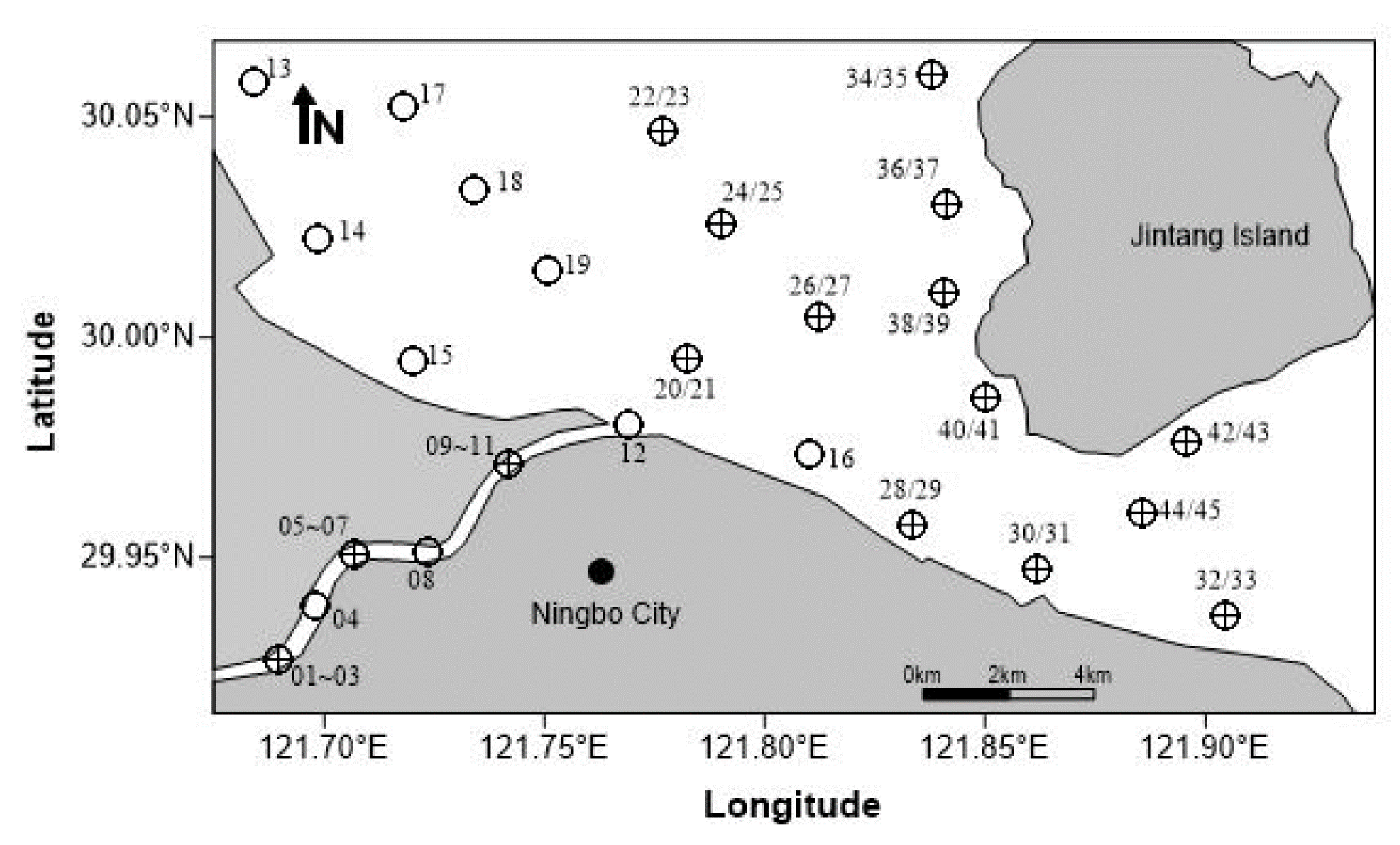
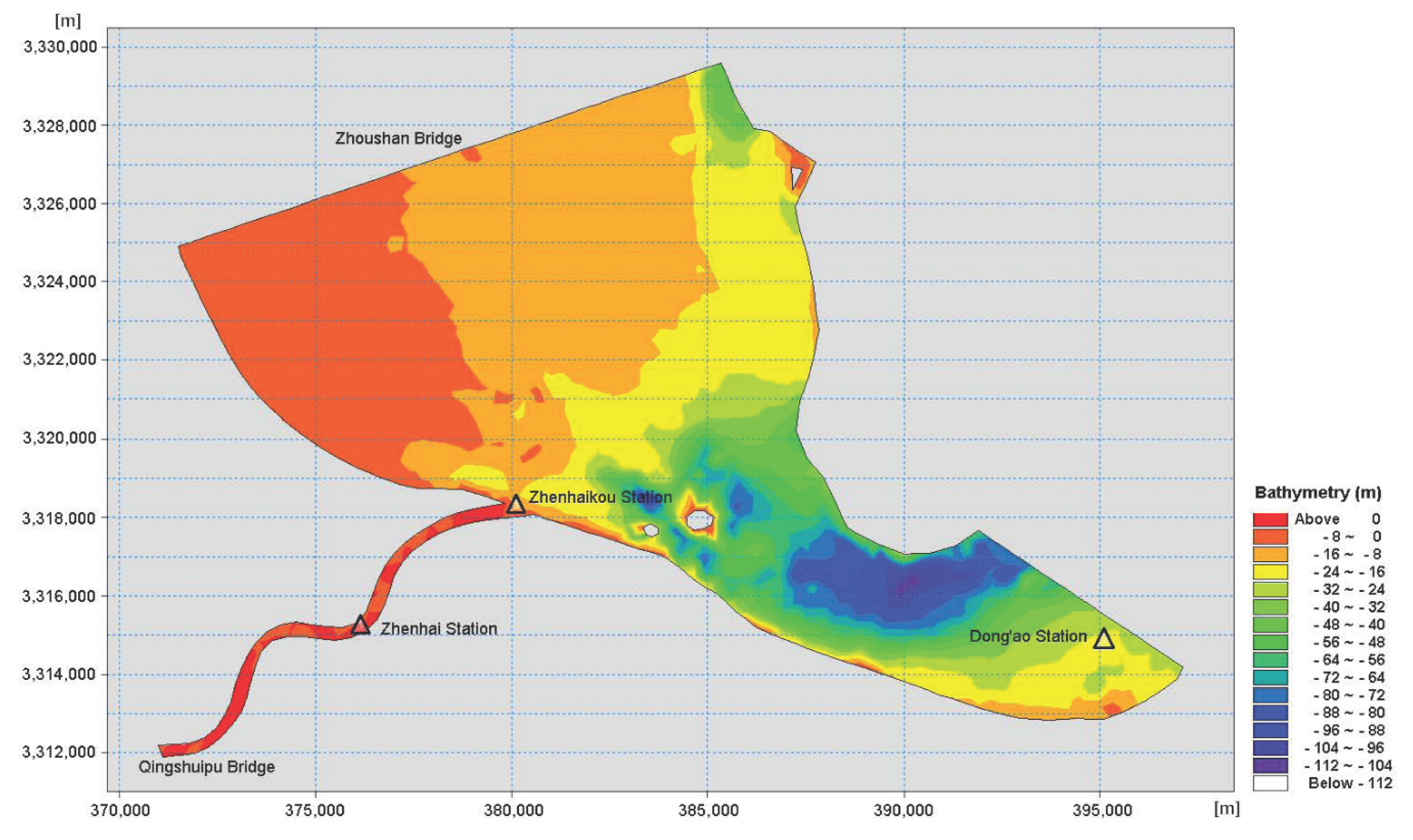
2.1. Description of Study Area

Yongjiang River, referring to the reach below Sanjiangkou in Ningbo city, stretches 25.6 km long with its drainage area of 3857.2 km² and a slope of 0.0117‰. The Yongjiang estuary faces Huibie Sea at Hangzhou Bay in the north, Jintang and Zhoushan Islands in the east. Its southeastern sea is Luotou Waterway. With a total riverbank line of 60km, it extends from northwest to southeast. The study area is shown in Figure 1.

The Yongjiang basin has a subtropical humid monsoon climate with an obvious change between winter and summer monsoons. The wind direction is southeast in summer and northwest in winter. The Yongjiang tide is an irregular semi-diurnal tide, with an annual maximum tide level of 4.86 m, a minimum of 0.13 m, an annual average high tide level of 3.14 m, a low level of 1.46 m and an average tide difference of 1.82 m.

2.2. Data Collection

Data of hydrology, water quality and biology of the study area involved in this paper were provided by Bureau of Hydrology and Water Resources Investigation at Lower Reaches of Yangtze River, Hydrology Bureau of Yangtze River Water Conservancy Commission, and came from the measurements carried out in June 2015 at sampling locations presented in Figure 2.

In Figure 2, there were 45 sampling points in total, 12 in the lower reach of the Yongjiang River (with numbers 1 through 12). From these 12, 9 were taken from three cross-sections, sampled evenly along the section three times (e.g., 01~03, marked with “⊕”). The other 33 points (with numbers 13 through 45) were taken in 20 locations in the estuary, with 13 locations sampled in both upper and lower water (e.g., 20/21, marked with “⊕”) thus representing 26 points. The other single sampling locations were marked with “◯” in Figure 2.

After the phytoplankton samples were collected, they were immediately fixed with Luge’s solution (usually 10 mL per liter of water). Then each sample was concentrated to 30~50 mL and poured into the calibrated precipitator. After 24~48 h, the supernatant was siphoned off. The sample could be stored in the sample bottle until it was concentrated to 30~50 mL. The types of samples were identified directly under the microscope and recorded. Their numbers were counted and calculated by microscope counting method.

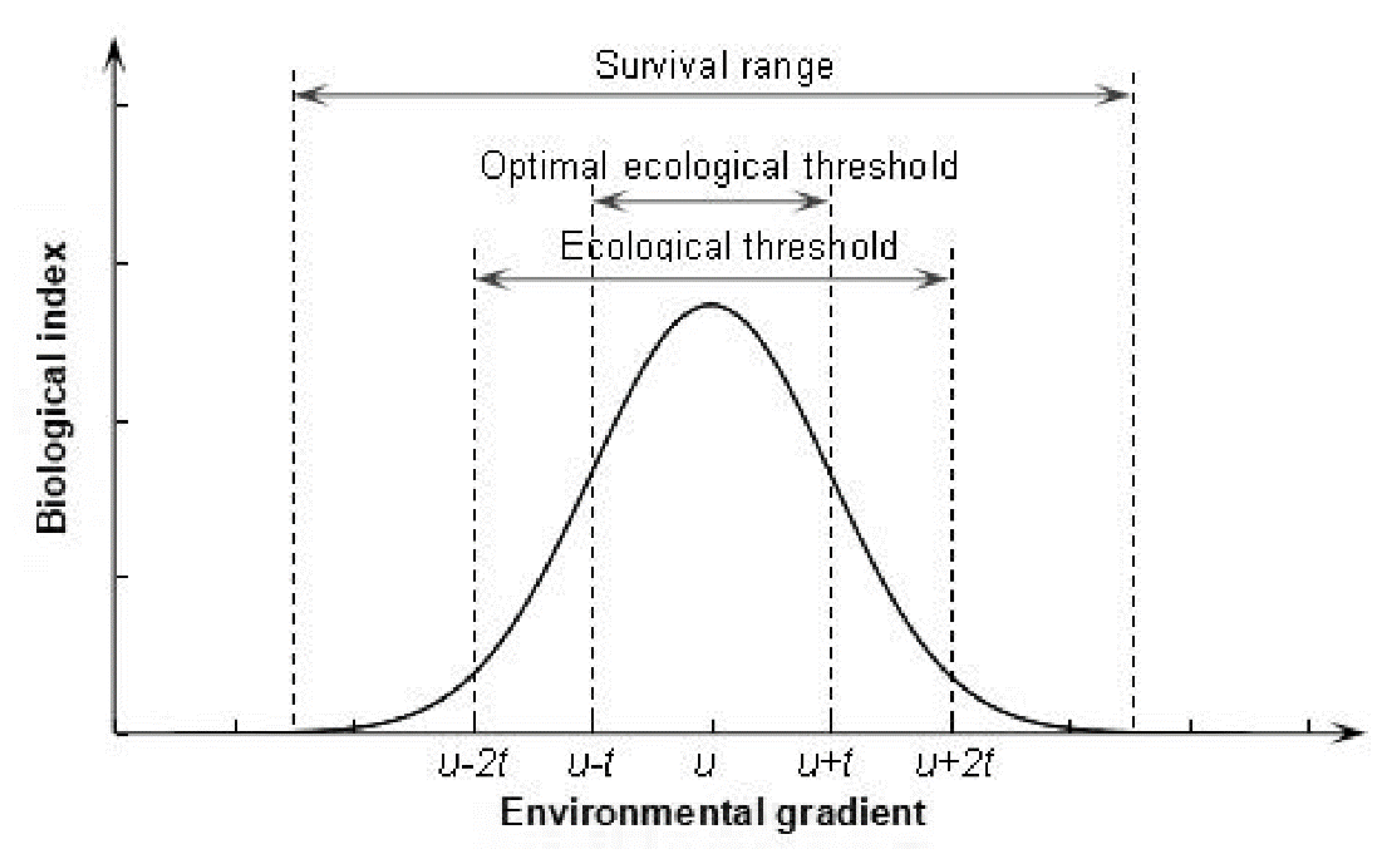
2.3. ET and Gaussian Curve Theory

Most ET studies focus on the known single environmental factor that can directly affect aquatic communities [15]. The determination of the ET zone is inseparable from Shelford’s Law of tolerance [30]. In Shelford’s thought, an organism’s adaptation to various environmental factors has its ecological minimum and maximum, between which the organism can survive. The organism’s function has its best performance at or near the optimum point, fading towards both endpoints and finally suppressed at those endpoints.

The relationship between organism and environmental factors is usually described by the bell-tolerance curve, matching the concentration, symmetry and even variability of the one-dimension Gaussian curve. Therefore, this paper simulated the above relationship and presented an ET zone range by using a Gaussian curve.

The one-dimension Gaussian model Equation is:

$$y=c\exp \left[-\frac{1}{2}{(x-u)}^2/t^2\right]$$

(1)

In the Equation, $y$ refers to one index that represents phytoplankton growth condition; $c$ is the maximum value of corresponding index; $u$ is the corresponding environmental factor value when its biological index reaches the maximum value; $t$ means the tolerance of the index, which describes biological species’ ecological threshold. Generally speaking, one biological specie’s ET zone is $\left(u-2t, u+2t\right)$, and its optimum ET zone is $\left(u-t, u+t\right)$. Figure 3 shows the Gaussian curve.

2.4. Ecological Factor Selection

Ecological factor is the general term of various environmental factors that influence organisms. A large number of studies indicate that phytoplankton growth, its community structure changes and regional distribution are affected by many environmental factors such as dissolved oxygen, salinity, nutrient salts, water temperature, and PH value [31,32,33,34,35]. A Pearson Correlation Analysis was made on the main environmental factors in the Yongjiang estuary. The result (see Table S1 in the Supplementary Materials section) indicates that there is no obvious correlation between them despite their respective influence on phytoplankton growth. In other words, their influence on phytoplankton can be regarded as independent. Therefore, a preliminary study of phytoplankton ET under salinity changes is undertaken in this paper. In most cases, salinity is a significant factor in the estuarine system controlling phytoplankton’s activity and diversity [36]. Sluice and dam construction will become a physical barrier to nutrient transport and will inevitably change the original salinity field in the estuary [10,36].

2.5. Numerical Simulation by MIKE 21 Software (DHI, Denmark)

Two-dimensional and three-dimensional numerical simulations have been widely applied in hydrology and water quality simulations of rivers, estuaries, and oceans [37,38,39,40,41,42,43]. MIKE 21(DHI, Denmark) is a professional engineering software to simulate hydrodynamic force, water quality, sediment and wave, which has advanced pre-processing and post-processing function and a friendly customer page and enjoys popularity in simulating water current, wave, sediment, and other environmental variables of river, lake, estuary, bay, coast, and ocean.

The following equations, the conservation of mass and momentum integrated over the vertical, describe the flow and water level variations:

(1)

Continuity Equation of water flow:

$$\frac{\partial z}{\partial t}+\frac{\partial M}{\partial x}+\frac{\partial N}{\partial y}=0$$

(2)

(2)

Momentum Equations pf water flow:

$$\frac{\partial u}{\partial t}+u\frac{\partial u}{\partial x}+v\frac{\partial u}{\partial y}+g\frac{\partial z}{\partial x}+g\frac{u\sqrt{u^2+v^2}}{c^{2}h}=v_t\left(\frac{{\partial }^{2}u}{\partial x^2}+\frac{{\partial }^{2}u}{\partial y^2}\right)$$

(3)

$$\frac{\partial v}{\partial t}+u\frac{\partial v}{\partial x}+v\frac{\partial v}{\partial y}+g\frac{\partial z}{\partial y}+g\frac{v\sqrt{u^2+v^2}}{c^{2}h}=v_t\left(\frac{{\partial }^{2}v}{\partial x^2}+\frac{{\partial }^{2}v}{\partial y^2}\right)$$

(4)

In the Equation:

• $x$, $y,$ and $t$ are the space and time coordinates respectively; $z$ is water level;
• $u$ and $v$ are the components of vertical mean velocity in the direction of $x$ and $y$ respectively;
• $M$ and $N$ are the components of discharge per unit width in the directions of $x$ and $y$;
• $M=hu$, $=hv$; $n$ is the Manning roughness coefficient;
• $c$ is the Chezy coefficient, $c=\frac{1}{n}{h}^{\frac{1}{6}}$;
• $v$_t is the turbulent viscosity coefficient; $g$ is the gravitational acceleration.

2.5.1. Model Establishment and Parameter Calibration

Simulation range covered the area from the Qingshuipu Bridge section along the Yongjiang trunk stream to the Zhoushan Bridge, Dong’ao offshore. UTM-51 was chosen as the projection zone. A Flow Model (FM) triangular mesh was applied to divide the calculation area, forming 2422 mesh triangles and 1606 mesh vertexes. The bathymetric topographic map (1:2000) of Yongjiang estuary in June 2015 was used for interpolation calculation of meshes and for obtaining the bathymetric map of the model (Figure 4).

The hydrodynamic module was calculated by low order of accuracy, in which calculation time was from 08:00:00 16 June 2015 to 08:00:00 26 June 2015; time step was set to 3600s, CFL numbers of the shallow water Equation and the transport Equation were all set to 0.8 to control equation convergence. The upstream boundary was measured by the water level at Qingshuipu Bridge in the same period, and the downstream boundary was the deep sea. The Global Tide Prediction Model programmed in MIKE 21 (DHI, Denmark) was applied to create a tidal water level. After calibration, the value of eddy viscosity coefficient was set to 0.7 and manning coefficient was set to 60 m^1/3/s. The Transport Module predefined in the software was selected to simulate salinity.

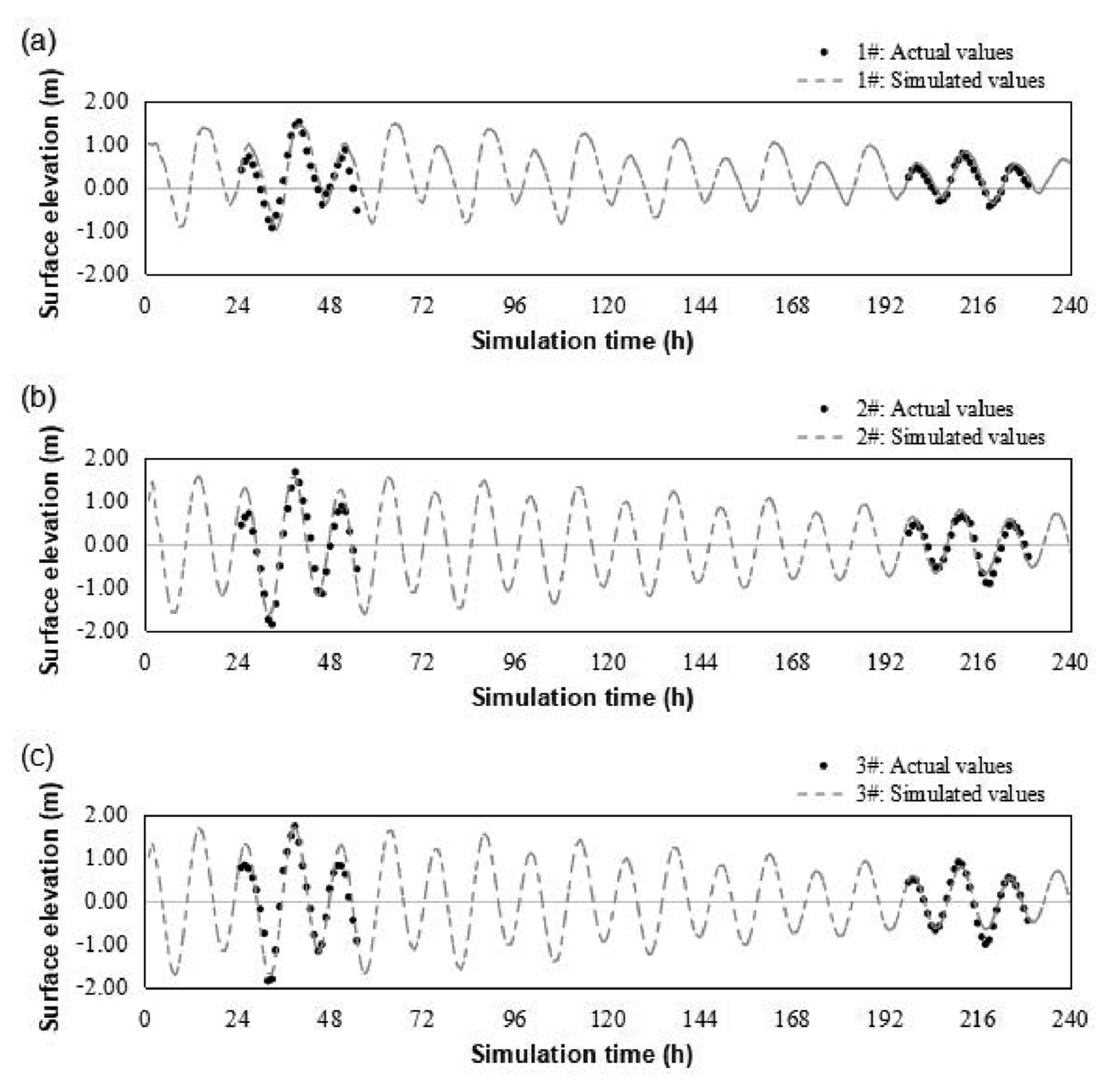
2.5.2. Tide Level Verification

The measured tide level values of the spring tide on 18 June 2015 and neap tide on 24 June 2015 were selected to verify those of the Zhenhai, Zhenhaikou, and Dong’ao observation stations (Figure 4).

2.5.3. Current Velocity Verification

The measured current velocity of the neap tide on 24 June 2015 was selected to verify the current velocity and flow direction at three observation points in the offshore area.

The offshore sea current compound is composed of the tidal current, wind current, and geostrophic current. It can be divided into periodic tidal current and non-periodic residual current. Therefore, the measured current velocity values could not be used for verification directly. A tidal current quasi-harmonic analysis according to short-term measured values was needed to predict tidal current values. The quasi-harmonic analysis uses a linear equation to analyze and calculate the northward and eastward components of tidal currents, solving tidal harmonic constants and residual current of partial tide by the least square method to present the north component u and the east component v at a designated time [44]. The harmonic constants of the tides selected by the quasi-harmonic analysis were used to forecast the flow corresponding to the simulation time for verification.

2.5.4. Sluice Construction Simulation

There are studies related to sluice construction practicability and analysis of sluice site selection in Yongjiang already in China [45]. Based on them, this paper selected the ESTUARY GATE scheme. The upper boundary hydrological condition adopted the monthly lowest average flow of 90% assurance rate, 4.12 m³/s, which was calculated by monthly average flow from 1985 to 2014 at the nearby Hongjiata station. The gate was set as a full water column considering the tide-resisting performance at the sluice site.

3. Results

3.1. Results of Sample Analysis

After preliminary identification, 53 kinds of phytoplankton were found in the study areas, in which there were 23 green algae covering 43.4% of total kinds, 12 blue-green algae covering 22.6%, and 11 diatoms covering 20.8%. The algae belonging to Bacillariophyta, Cyanophyta and Chlorophyta (e.g., Oscillaria sp, Melosira granulata, Tribonema Derbes et Solier, Microcystis aeruginisa, Pediastrum semplex) have the highest percentage in cell density.

3.2. Results of Water Level and Velocity Verification

3.2.1. Results of Water Level Verification

After calculation, the result shows that the average relative errors between measured tide level and the simulated value at the three tide stations are within the range of 3.3–4.4% during the spring tide and between 2.4–3.8% during the neap tide, meeting the simulation requirements.

Comparison between simulated water level and the measured water level is shown in Figure 5. The simulated water level values are basically consistent with the measured water level values at each station.

3.2.2. Results of Velocity Verification

Based on the quasi-harmonic analysis, tidal current matching the simulation time is predicted by harmonic constants of partial tide K1, M2, M3, M4, 2MK5, M6, 3MK7, M8.

After calculation, the average relative errors between the simulated values and the measured values of flow velocity and direction at the three observation stations are within the range of 1.6–3.8% during the neap tide, which meet the simulation requirements.

3.3. Results of Salinity Simulation

The average values of salinity during the simulation period in the estuary are introduced to Surfer15, interpolated by the Kriging method to draw contour plots. The two contour plots of salinity gradient changes before and after sluice construction are shown in Figure 6. Contour map (a) was drawn with the measured data and contour map (b) was generated with the simulated data when a gate was added at the entrance to the estuary. The sampling points in the estuary (with number 13 through 45) were marked in both maps to analyze the salinity changes in these locations.

3.4. ET Calculation

Natural logarithms are taken on both sides of the Equation (1) to get the quadratic Equation (5), where $a_0=\ln c-\frac{u^2}{2t^2}$, $a_1=\frac{u}{t^2}$, $a_2=-\frac{1}{2t^2}$

$$F\left(x\right)=a_0+a_{1}x+a_{2}x$$

(5)

The result of a quadratic fitting of Equation (5) and the measured salinity values is: $y=-0.432x^2+17.92x-162$ (R² = 0.839). The fitting curve is shown in Figure 7.

Based on the transformation relationship between the fitted quadratic equation and Gaussian model, Gauss Equation is solved as:

$$f\left(x\right)=20.57\times {10}^4\exp \left[-\frac{1}{2}(x-20.91{)}^2/{1.08}^2\right]$$

(6)

According to the Equation, optimum value u is 20.91‰, ET zone is (18.75, 23.07) (‰), optimum ET zone is (19.83, 21.99) (‰).

3.5. Descriptive Analysis of Salinity Values

Descriptive analysis of salinity values in 2422 computational meshes in the study area before and after sluice construction was conducted. The results are shown in

Table 1. Descriptive analysis of salinity (‰).

Statistical Indicator	No Gate	Estuary Gate
Minimum	13.776	15.239
Maximum	23.643	24.021
Mean	22.137	23.146
Median	22.256	23.179
Geometric Mean	21.970	23.102
Harmonic Mean	21.590	23.046
Root Mean Square	22.221	23.181
Trim Mean (10%)	22.351	23.292
Variance	3.744	1.622
Standard Deviation	1.935	1.273

.

Before sluice construction, the salinity range in Yongjiang offshore sea water varied roughly from 21.7 to 23.6‰, as shown in Figure 6a, while the low salinity values were concentrated in the river channel area with a minimum salinity of 13.776‰, as shown in Table 1.

4. Discussion and Conclusions

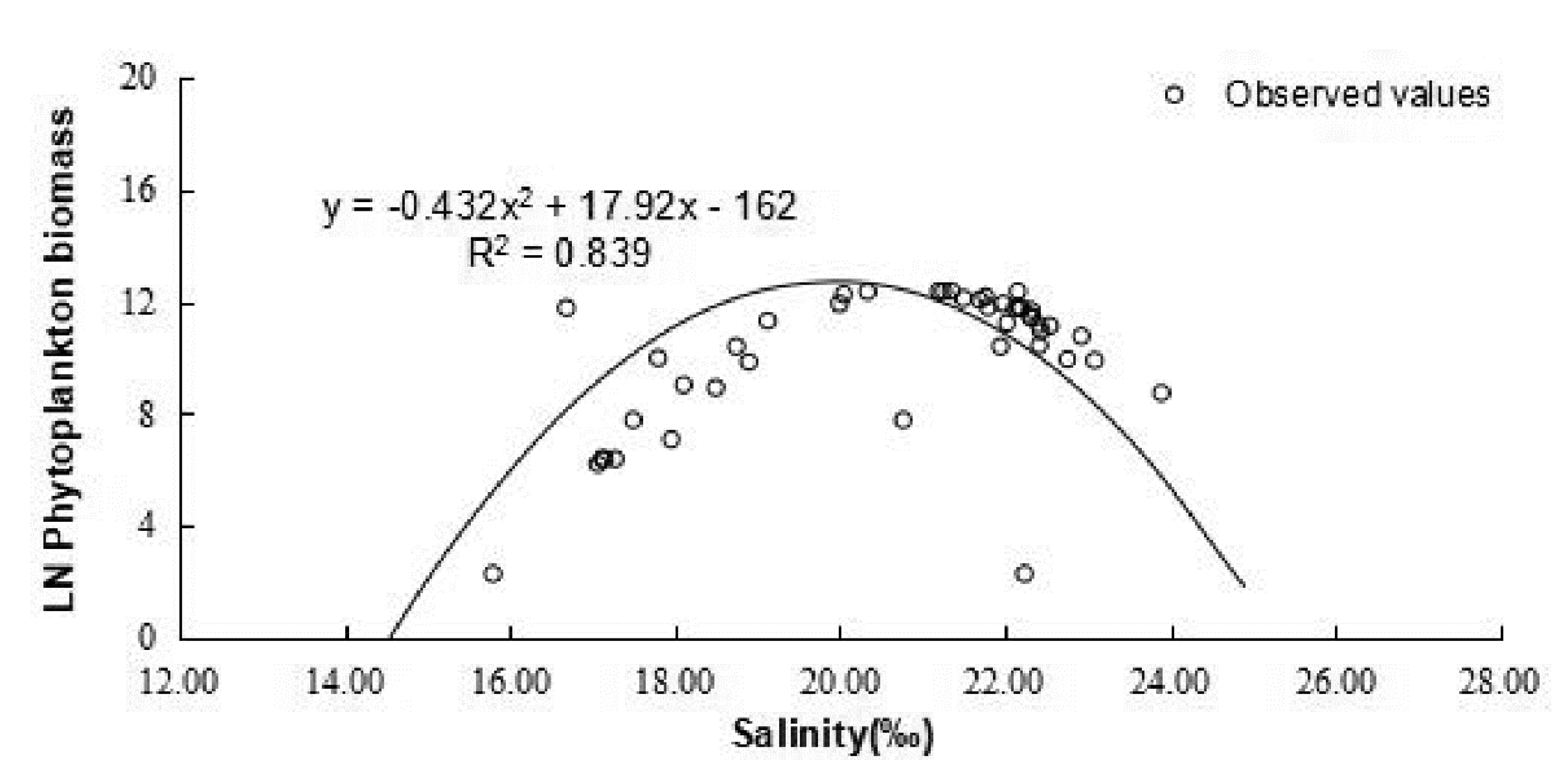
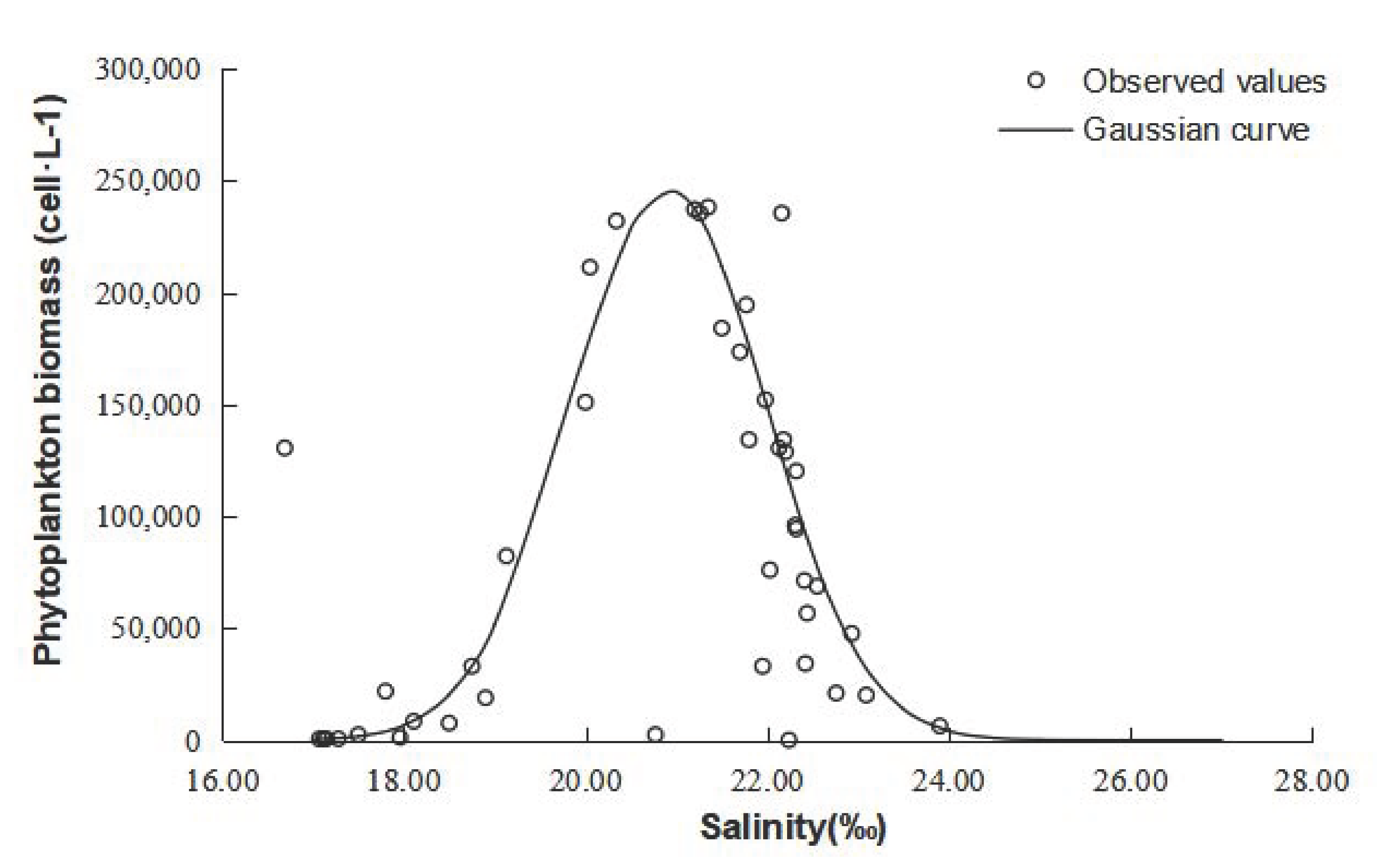
4.1. Checking of Gaussian Curve

Based on the fitted one-dimension Gaussian Equation curve, a comparison can be drawn between measured phytoplankton cell density and Gaussian model theoretical values. As shown in Figure 8, the changing trend of the Gaussian model is consistent with that of the measured values, which suggests that the relationship between phytoplankton and salinity can be well described by the Gaussian Equation as calculated. Thus, the threshold zone (18.75, 23.07) (‰) of salinity calculated in this paper is adequately representative of the appropriate salinity condition to which phytoplankton growth is subject in the Yongjiang estuary.

The Gaussian Equation also shows its reasonability in the ET studies of species in other regions. Baoshan Cui et al. adopted Suaeda salsa (L.) Pall. biomass as an index to study the ET of the Suaeda salsa (L.) Pall. community under the scope of changes in water depth and soil salinity in the Yellow River Delta. The authors applied a Gaussian model, which revealed that the water depth in the ET zone of Suaeda salsa (L.) Pall. ranged (−0.92, 0.08) (m), and that salinity in the ET zone ranged (5.17, 20.25) (g/kg). Furthering this, a discussion was conducted around the potential impact of water–salt interaction on Suaeda salsa (L.) Pall. growth [46]. By taking the Gaussian model approach, Yiyi Yang et al. conducted a study on the relationship between phytoplankton cell density and various environmental factors at the Yueqing Bay located in Zhejiang Province, China, which is close to the Yongjiang River. It was found that the salinity in the ET zone fell within the range of (24.36,27.88) (‰), with an optimum ET range of (25.24,27.00) (‰), which is closely matched by the results obtained in this work [47]. Yi Li et al. analyzed the correlation between Labidocera euchaeta and the salinity of sea water in the same area as Yang, finding that Labidocera euchaeta ET zone under salinity gradient ranged (18.99,23.73) (‰) and optimum salinity ET zone was (20.17,22.55) (‰) [48]. Thus, it can be argued that applying the Gaussian curve for ET studies is effective to quantify biological tolerance.

4.2. Prediction of Phytoplankton Density

After sluice construction, salinity in the estuary showed an increase since the gate acted as a physical barrier to hinder the exchange between fresh water and sea water to some degree [10,36]. According to the simulation, the maximum salinity reached 24.021‰, up from 23.643‰, while the average value surged from 22.137‰ to 23.146‰. On average, the level of salinity increased by about 1% in the entire estuary after sluice construction. At the sample point 12#, there was a notable increase in salinity, by around 0.4‰, which was close to where the planned sluice was located. For the sample points 13–15# and 17–19#, which were near the Zhoushan Bridge, their salinity showed no notable increase, as it rose by merely 0.2‰. However, a high salinity region, covering sample points 16#, 28–33#, 38–45#, was concentrated in the south of the Jintang Island, where the level of salinity increased by 0.4–0.8‰, as shown in Figure 6.

According to the salinity the ET of phytoplankton solved by the Gaussian curve, when salinity in the Yongjiang estuary falls within the range of 18.75~23.07‰, phytoplankton survives. When salinity ranges between 19.83‰ and 21.99‰, phytoplankton is left in the optimum condition with a higher phytoplankton cell density. After the sluice construction, salinity in the estuary is much higher than the threshold range suitable for phytoplankton growth. According to the Gaussian curve, the salinity range in the western sea area of the Jintang Island is 23.0 ± 0.6‰, which is beyond the optimum range for phytoplankton growth and is close to the lethal point. Moreover, the salinity value in the southern sea area of the Jintang Island reached 24.021‰, which is also beyond the lethal point, thus making it difficult for phytoplankton to grow in this area after sluice construction. As diatom, green algae and blue-green algae are the dominant groups in the phytoplankton community before sluice construction, it is expected that the abundance of freshwater green algae, which ranks as top in the phytoplankton community in the Yongjiang estuary, will be reduced significantly, while the brackish water algae (e.g., the diatom) may be subjected to only limited impact. Since the quantity of phytoplankton is an essential index for the evaluation of primary productivity, it is foreseeable that it will show a decreasing trend in the estuary after sluice construction.

4.3. Limitation and Prospect

The ET of phytoplankton solved in this paper is limited to targeting the environmental gradient of salinity of the study area. There is the possibility that the sluice construction may affect other hydrological and nutritional factors to varying degrees, as a result of which the accuracy of the ET zone may be compromised to some extent. Besides, multiple sampling in a location is also a limitation imposed on this study. There may be autocorrelation biases of the sampling points on the same cross-section, as they are much closer to each other than the overall sampling points. The points sampled at different depths in the estuary are also the potential influencing factors for the results.

The estuarine ecosystem is highly complex in structures, which makes it necessary to conduct more systematic and comprehensive studies on ET. Based on the results obtained in this work, the dominant phytoplankton species on different nutritional levels in the estuarine ecosystems should be monitored in future research. Besides, the number of samples should be increased and the sampling locations ought to be distributed in a more sensible way. More accurate indoor breeding experiments can be conducted to study the micro physiological response of phytoplankton to the water–salt gradient and its ET under other environmental gradients. Only in this way can the state of the ecosystem be better understood.

References

1. Litchman, E.; Pinto, P.D.; Edwards, K.F.; Klausmeier, C.A.; Kremer, C.T.; Thomas, M.K. Global biogeochemical impacts of phytoplankton: A trait-based perspective. J. Ecol. 2015, 103, 1384–1396. [Google Scholar] [CrossRef] [Green Version]
2. Goldyn, H. Changes in plant species diversity of aquatic ecosystems in the agricultural landscape in West Poland in the last 30 years. Biodivers. Conserv. 2010, 19, 61–80. [Google Scholar] [CrossRef]
3. Caroppo, C. Ecology and biodiversity of picoplanktonic cyanobacteria in coastal and brackish environments. Biodivers. Conserv. 2015, 24, 949–971. [Google Scholar] [CrossRef]
4. Peter, P.O.; Rashid, A.; Hou, L.; Nkinahamira, F.; Kiki, C.; Sun, Q.; Yu, C.-P.; Hu, A. Elemental contaminants in surface sediments from jiulong river estuary, china: Pollution level and ecotoxicological risk assessment. Water 2020, 12, 1640. [Google Scholar] [CrossRef]
5. Lepisto, L.; Holopainen, L.L.; Vuoristo, H. Type-specific and indicator taxa of phytoplankton as a quality criterion for assessing the ecological status of Finnish boreal lakes. Limnologica 2004, 34, 236–248. [Google Scholar] [CrossRef] [Green Version]
6. Rojo, C.; Alvarez-Cobelas, M.; Benavent-Corai, J.; Baron-Rodriguez, M.M.; Rodrigo, M.A. Trade-offs in plankton species richness arising from drought: Insights from long-term data of a National Park wetland (central Spain). Biodivers. Conserv. 2012, 21, 2453–2476. [Google Scholar] [CrossRef]
7. Rath, A.R.; Mitbavkar, S.; Anil, A.C. Phytoplankton community structure in relation to environmental factors from the New Mangalore Port waters along the southwest coast of India. Environ. Monit. Assess. 2018, 190. [Google Scholar] [CrossRef]
8. Thackeray, S.J.; Jones, I.D.; Maberly, S.C. Long-term change in the phenology of spring phytoplankton: Species-specific responses to nutrient enrichment and climatic change. J. Ecol. 2008, 96, 523–535. [Google Scholar] [CrossRef]
9. Whitehead, P.G.; Bussi, G.; Bowes, M.J.; Read, D.S.; Hutchins, M.G.; Elliott, J.A.; Dadson, S.J. Dynamic modelling of multiple phytoplankton groups in rivers with an application to the Thames river system in the UK. Environ. Model. Softw. 2015, 74, 75–91. [Google Scholar] [CrossRef]
10. Mousing, E.A.; Richardson, K.; Bendtsen, J.; Cetinic, I.; Perry, M.J. Evidence of small-scale spatial structuring of phytoplankton alpha- and beta-diversity in the open ocean. J. Ecol. 2016, 104, 1682–1695. [Google Scholar] [CrossRef]
11. Santos, J.M.; Ferreira, M.T. Use of aquatic biota to detect ecological changes in freshwater: Current status and future directions. Water 2020, 12, 1611. [Google Scholar] [CrossRef]
12. Zhao, G.; Pan, B.; Li, Y.; Zheng, X.; Zhu, P.; Zhang, L.; He, H. Phytoplankton in the heavy sediment-laden Weihe River and its tributaries from the northern foot of the Qinling Mountains: Community structure and environmental drivers. Environ. Sci. Pollut. Res. Int. 2020, 27, 8359–8370. [Google Scholar] [CrossRef] [PubMed]
13. Huggett, A.J. The concept and utility of ’ecological thresholds’ in biodiversity conservation. Biol. Conserv. 2005, 124, 301–310. [Google Scholar] [CrossRef]
14. Baker, M.E.; King, R.S. A new method for detecting and interpreting biodiversity and ecological community thresholds. Methods Ecol. Evol. 2010, 1, 25–37. [Google Scholar] [CrossRef]
15. Roubeix, V.; Danis, P.A.; Feret, T.; Baudoin, J.M. Identification of ecological thresholds from variations in phytoplankton communities among lakes: Contribution to the definition of environmental standards. Environ. Monit. Assess. 2016, 188. [Google Scholar] [CrossRef] [Green Version]
16. Groffman, P.; Baron, J.; Blett, T.; Gold, A.; Goodman, I.; Gunderson, L.; Levinson, B.; Palmer, M.; Paerl, H.; Peterson, G.; et al. Ecological thresholds: The key to successful environmental management or an important concept with no practical application? Ecosystems 2006, 9, 1–13. [Google Scholar] [CrossRef]
17. Muradian, R. Ecological thresholds: A survey. Ecol. Econ. 2001, 38, 7–24. [Google Scholar] [CrossRef]
18. With, K.A.; King, A.W. Extinction thresholds for species in fractal landscapes. Conserv. Biol. 1999, 13, 314–326. [Google Scholar] [CrossRef]
19. Fahrig, L. How much habitat is enough? Biol. Conserv. 2001, 100, 65–74. [Google Scholar] [CrossRef]
20. Soranno, P.A.; Cheruvelil, K.S.; Stevenson, R.J.; Rollins, S.L.; Holden, S.W.; Heaton, S.; Torng, E. A framework for developing ecosystem-specific nutrient criteria: Integrating biological thresholds with predictive modeling. Limnol. Oceanogr. 2008, 53, 773–787. [Google Scholar] [CrossRef] [Green Version]
21. Andersen, T.; Carstensen, J.; Hernandez-Garcia, E.; Duarte, C.M. Ecological thresholds and regime shifts: Approaches to identification. Trends Ecol. Evol. 2009, 24, 49–57. [Google Scholar] [CrossRef] [Green Version]
22. Catalan, J.; Barbieri, M.G.; Bartumeus, F.; Bitusik, P.; Botev, I.; Brancelj, A.; Cogalniceanu, D.; Manca, M.; Marchetto, A.; Ognjanova-Rumenova, N.; et al. Ecological thresholds in European alpine lakes. Freshwater Biol. 2009, 54, 2494–2517. [Google Scholar] [CrossRef]
23. Basang, W.D.; Zhu, Y.B. Whole-genome analysis identifying candidate genes of altitude adaptive ecological thresholds in yak populations. J. Anim. Breed. Genet. 2019, 136, 371–377. [Google Scholar] [CrossRef]
24. Wolski, K.; Tymiński, T. Studies on the threshold density of Phragmites australis plant concentration as a factor of hydraulic interactions in the riverbed. Ecol. Eng. 2020, 151. [Google Scholar] [CrossRef]
25. Kanaya, G.; Nakamura, Y.; Koizumi, T. Ecological thresholds of hypoxia and sedimentary H2S in coastal soft-bottom habitats: A macroinvertebrate-based assessment. Mar. Environ. Res. 2018, 136, 27–37. [Google Scholar] [CrossRef]
26. Daily, J.P.; Hitt, N.P.; Smith, D.R.; Snyder, C.D. Experimental and environmental factors affect spurious detection of ecological thresholds. Ecology 2012, 93, 17–23. [Google Scholar] [CrossRef] [Green Version]
27. Cui, Y.P. Preliminary estimation of the realistic optimum temperature for vegetation growth in China. Environ. Manag. 2013. [Google Scholar] [CrossRef]
28. Wen, S.Y.; Song, L.L.; Long, H.; Yu, J.; Gao, S.G.; Zhao, D.Z. Nutrient-based method for assessing the hazard degree of red tide: A case study in the zhejiang coastal waters, east china sea. Environ. Earth Sci. 2013, 70, 2671–2678. [Google Scholar] [CrossRef]
29. McDonald, K.S.; Tighe, M.; Ryder, D.S. An ecological risk assessment for managing and predicting trophic shifts in estuarine ecosystems using a Bayesian network. Environ. Model. Softw. 2016, 85, 202–216. [Google Scholar] [CrossRef]
30. Shelford, V.E. Physiological animal geography. J. Morphol. 1911, 22, 551–618. [Google Scholar] [CrossRef]
31. Thompson, P.A. Temporal variability of phytoplankton in a salt wedge estuary, the Swan-Canning Estuary, Western Australia. Hydrol. Process. 2001, 15, 2617–2630. [Google Scholar] [CrossRef]
32. Waylett, A.J.; Hutchins, M.G.; Johnson, A.C.; Bowes, M.J.; Loewenthal, M. Physico-chemical factors alone cannot simulate phytoplankton behaviour in a lowland river. J. Hydrol. 2013, 497, 223–233. [Google Scholar] [CrossRef]
33. Kouhanestani, Z.M.; Roelke, D.L.; Ghorbani, R.; Fujiwara, M. Assessment of spatiotemporal phytoplankton composition in relation to environmental Conditions of Gorgan Bay, Iran. Estuaries Coasts 2019, 42, 173–189. [Google Scholar] [CrossRef]
34. Li, X.Y.; Yu, H.X.; Wang, H.B.; Ma, C.X. Phytoplankton community structure in relation to environmental factors and ecological assessment of water quality in the upper reaches of the Genhe River in the Greater Hinggan Mountains. Environ. Sci. Pollut. Res. 2019, 26, 17512–17519. [Google Scholar] [CrossRef] [PubMed]
35. Van Meerssche, E.; Pinckney, J.L. Nutrient Loading Impacts on Estuarine Phytoplankton Size and Community Composition: Community-Based Indicators of Eutrophication. Estuaries Coasts 2019, 42, 504–512. [Google Scholar] [CrossRef]
36. Quinlan, E.L.; Phlips, E.J. Phytoplankton assemblages across the marine to low-salinity transition zone in a blackwater dominated estuary. J. Plankton Res. 2007, 29, 401–416. [Google Scholar] [CrossRef]
37. Zhang, D.; Han, D.; Song, X. Impacts of the Sanmenxia Dam on the Interaction between Surface Water and Groundwater in the Lower Weihe River of Yellow River Watershed. Water 2020, 12, 1671. [Google Scholar] [CrossRef]
38. Remya, P.G.; Kumar, R.; Basu, S.; Sarkar, A. Wave hindcast experiments in the Indian Ocean using MIKE 21 SW model. J. Earth Syst. Sci. 2012, 121, 385–392. [Google Scholar] [CrossRef] [Green Version]
39. VishnuRadhan, R.; Vethamony, P.; Zainudin, Z.; Kumar, K.V. Waste Assimilative Capacity of Coastal Waters along Mumbai Mega City, West Coast of India Using MIKE-21 and WASP Simulation Models. Clean Soil Air Water 2014, 42, 295–305. [Google Scholar] [CrossRef]
40. Kim, J.; Lee, T.; Seo, D. Algal bloom prediction of the lower Han River, Korea using the EFDC hydrodynamic and water quality model. Ecol. Model. 2017, 366, 27–36. [Google Scholar] [CrossRef]
41. Gao, Q.F.; He, G.J.; Fang, H.W.; Bai, S.; Huang, L. Numerical simulation of water age and its potential effects on the water quality in Xiangxi bay of three gorges reservoir. J. Hydrol. 2018, 566, 484–499. [Google Scholar] [CrossRef]
42. Waldman, S.; Baston, S.; Nemalidinne, R.; Chatzirodou, A.; Venugopal, V.; Side, J. Implementation of tidal turbines in MIKE 3 and Delft3D models of Pentland Firth & Orkney waters (vol 147, pg 21, 2017). Ocean Coast. Manag. 2018, 163, 535–536. [Google Scholar] [CrossRef]
43. Gou, H.; Luo, F.; Li, R.; Dong, X.; Zhang, Y. Modeling Study on the Hydrodynamic Environmental Impact Caused by the Sea for Regional Construction near the Yanwo Island in Zhoushan, China. Water 2019, 11, 1674. [Google Scholar] [CrossRef] [Green Version]
44. Pawlowicz, R.; Beardsley, B.; Lentz, S. Classical tidal harmonic analysis including error estimates in MATLAB using T-TIDE. Comput. Geosci. 2002, 28, 929–937. [Google Scholar] [CrossRef]
45. Lan, X.; Zhang, H.; Wang, J.; Xu, J. Environmental impacts of building sluice on river estuary of Zhejiang Province. Water Resour. Prot. 2015, 2, 83–87. (In Chinese) [Google Scholar]
46. Cui, B.; He, Q.; Zhao, X. Researches on the ecological thresholds of Suaeda salsa to the environmental gradients of water table depth and soil salinity. Acta Ecol. Sin. 2008, 28, 1408–1418. (In Chinese) [Google Scholar] [CrossRef]
47. Yang, Y.; Li, Y.; Ye, S. Studies on the ecological threshold of phytoplankton to the environmental gradient of salinity in the Yueqing bay, Zhejiang province, China. Mar. Environ. Sci. 2018, 37, 499–504. (In Chinese) [Google Scholar]
48. Li, Y.; Yang, Y.; Ye, S. Ecological thresholds of Labidocera euchaeta to the gradient of salinity in Yueqing Bay, Zhejiang. J. Appl. Oceanogr. 2019, 3, 393–398. (In Chinese) [Google Scholar]
Figure 1. The study area: The lower reach below the Sanjiangkou in Ningbo is the Yongjiang River. The Yongjiang estuary is north to Huibie Sea in Hangzhou Bay and east to Jintang Island.
Water 12 02492 g001
Figure 2. Sampling locations in the lower reach and the estuary of the Yongjiang River. The 26 locations account for 45 points, 12 in the lower reach of the river and 33 in the estuary. Of the 12 points, nine were taken from three cross-sections, sampled evenly along the section three times. The other 33 points (with numbers 13 through 45) were taken in 20 locations in the estuary, with 13 locations sampled in both upper and lower water. Single sampling points were marked with “◯” in their locations, while the multiple ones were marked with “⊕”.
Water 12 02492 g002
Figure 3. Gaussian curve and ecological threshold: u is the corresponding environmental factor value when the corresponding biological index reaches the maximum, and t is the tolerance of the index, which is an index to describe the ecological threshold of biological species. The ecological threshold interval of a biological species is [u − 2t, u + 2t], and the optimum ecological threshold interval is [u − t, u + t].The species can only survive in the survival range.
Water 12 02492 g003
Figure 4. The bathymetric map of the study area generated by MIKE 21 (DHI, Denmark). Zhenhai, Zhenhaikou, and Dong’ao are the observation stations.
Water 12 02492 g004
Figure 5. Tide Level Verification by comparison of simulated water level and the measured water level values at the three observation stations: Zhenhai (a), Zhenhaikou (b), and Dong’ao (c).
Water 12 02492 g005
Figure 6. Contour map of salinity: (a) Contour map of salinity drawn with the measured data; (b) Contour map of salinity generated with the simulated data when a gate was added at the entrance to the estuary. See Figure 2 for detailed information about sampling locations and points.
Water 12 02492 g006
Figure 7. Quadratic fitting of salinity: The quadratic curve y = 0.432 x 2 + 17.92 x 162 fits well with the natural logarithm of measured phytoplankton cell density. R2 value is 0.839.
Water 12 02492 g007
Figure 8. Gaussian curve and observed values: The Gaussian curve drawn according to Equation (6) fitted well with actual phytoplankton biomass and could adequately illustrate the tolerance of phytoplankton to the salinity.
Water 12 02492 g008