Numerical Modelling and Simulation of Two-Phase Flow Flushing Method for Pipeline Cleaning in Water Distribution Systems

Abstract

Secondary pollution by microorganisms and substances peeling off from the “growth ring” causes clean water deterioration during the water distribution process. In order to reduce the secondary pollution, our previous research investigated the best settings of a two-phase flow flushing method for pipeline cleaning in water distribution systems experimentally, and a case study was carried out for comparison of the efficiencies between two-phase and single-phase flow methods. In this paper, based on the results of the experimental study, numerical modelling and a simulation study are carried out by FLUENT to evaluate the performance of the two-phase flow flushing method for removal of the “growth ring”. Results: the simulation results match the experimental results; pressure, water-phase flow velocity and water-phase volume ratio distributions in a section of pipe are simulated and analysed; the shear force against time in a period is obtained; elbow pipes cause flushing energy loss, and therefore, at most one section of elbow pipe is flushed in one flushing period.

1. Introduction

Although water delivered from a treatment plant is required to meet clean water standard initially, long-distance travel leads to the deterioration of clean water because of secondary pollution by microorganisms and substances peeling off from the “growth ring” into bulk water. The attached sediments on the pipe wall can react with pipe wall materials through chemical, electrochemical or biochemical processes to form an irregular “growth ring” towards the pipe centre [1,2,3,4,5,6]. This process is extremely harmful to drinking water quality.

Generally, the “growth ring” consists of three layers: a biological membrane layer, deposition layer and corrosion layer [6]. This three-layer structure provides an environment for bacterial growth, and the grown bacteria further promotes metal corrosion [7]. Sanitisers are utilised to control the growth of microorganisms, but sanitiser residuals can promote a corrosion reaction [8]. These factors make the “growth ring” widely formed in current cast iron water distribution pipelines.

The “growth ring” also severely damages water distribution pipelines themselves because its growth occupies the room for water distribution. This leads to unplanned pressure increases and unwanted vibrations in pipes. The corroded pipe walls become more fragile than normal. The aforementioned factors facilitate the emergence of drinking water leakages. These leakages cause drinking water loss, energy wastes, and contamination to the clean water. Consequently, they can even threaten end users’ health. Therefore, effective and timely removal of the “growth ring” in water distribution pipelines is a key issue to maintain drinking water quality [6].

A two-phase flow flushing method for removal of the “growth ring” has been studied theoretically by Wang et al. [9]. They did a simulation to theoretically analyse the two-phase flow flushing mechanisms in the water distribution pipes. In our previous research [10], an experimental study of two-phase flow flushing for the removal of the “growth ring” in water distribution systems has been carried out. It concluded the best settings of two-phase flow flushing method and laid a concrete foundation to carry out further multi-phase flow flushing investigations. Coronado-Hernández, O.E. et al. and Besharat, M. et al. [11,12,13,14,15,16,17,18,19] undertook in depth analysis on the effects of air–water two-phase flow in the water distribution pipes. They utilised both experiments and numerical simulations to analyse air–water two-phase flow from a variety of views and with case studies.

This paper will further investigate the two-phase flow flushing method for efficient removal of the “growth ring”. It will use numerical modelling and simulation to analyse the two-phase flow flushing method by FLUENT. The rest of the paper is organized as follows. Section 2 is the experiments. Section 3 is numerical modelling and simulation analysis. Finally, in Section 4, the paper is concluded.

2. Experiments

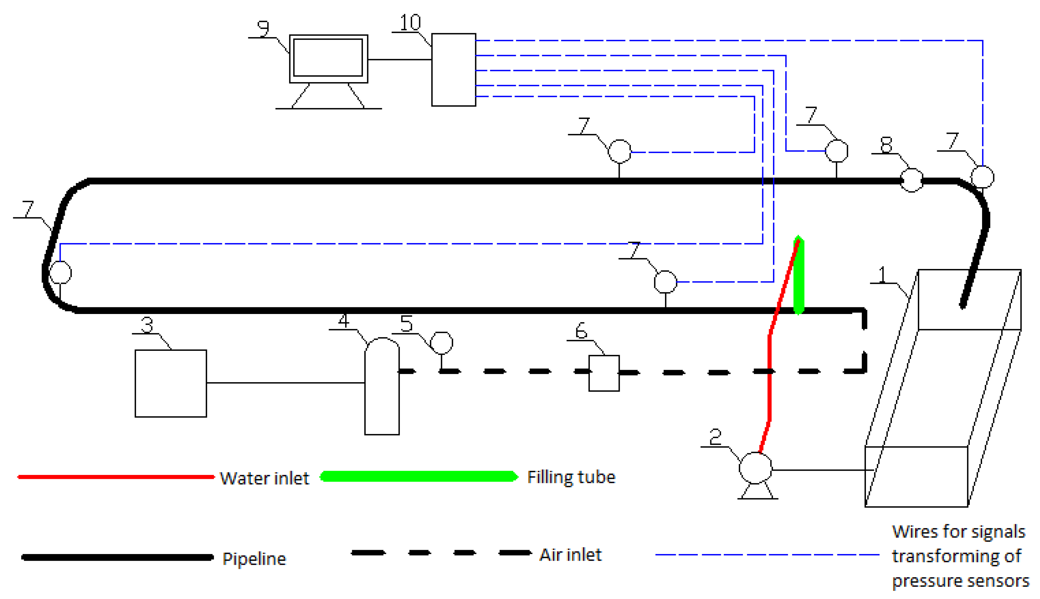
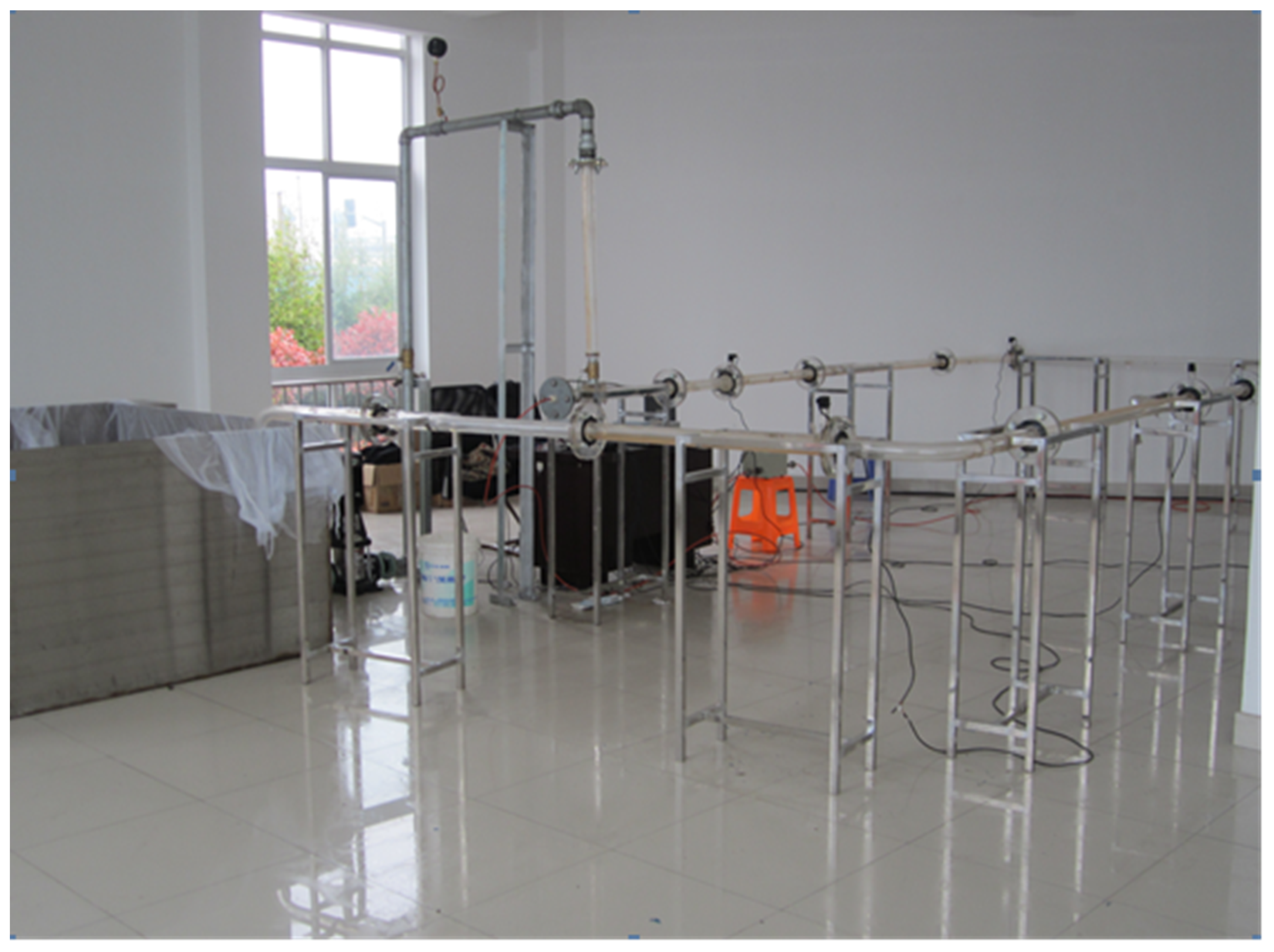
2.1. Experimetal Setup

Figure 1 is the experimental setup with the names of all components. Figure 2 is the photo of the experimental setup in the laboratory. The pipe wall is made of polymethyl methacrylate. The entire pipe is formed of parts connecting with each other using flanges. The internal diameter of the pipe is 40 mm, and the external diameter is 60 mm. The size of the water tank is 2000 mm × 2000 mm × 1000 mm. The entire experimental framework consists of a circulatory water supply system, an air supply system, and an experimental pipeline with a data acquisition system.

The water pump draws the water from the water tank. The valve controls the flow rate. The measurement of the flow rate is carried out by the flow meter. The air compressor compresses the input air. The gasholder controls the air pressure. During all experiments, the pipe should be strictly sealed. The pumped-out water and the compressed air are mixed in a T joint and then flow into the water tank along the pipe. Finally, water flows into the water tank for cycle use.

2.2. Experimental Results

Based on the results of the two-phase flow flushing experiment, the best settings (pulse frequency, nozzle shape, nozzle location) have been confirmed [10]: a round air inflow nozzle at the bottom of the pipe operates at 4–6 s (air inflow time is 4 s and air cut off time is 6 s). By using these settings, the amplitude of the pressure fluctuation and flow velocity reach the highest, i.e., the flushing effect is the best.

3. Numerical Modelling and Simulation

3.1. Mathmatical Modelling

3.1.1. Turbulent Flow Modelling

During air–water two-phase flow pipeline flushing, the Reynolds number of the water phase is far greater than critical Reynolds number. Its flow movement can be judged as turbulent flow. The turbulent flow equation selects the standard $k$ –$\epsilon$ model in this work. Therefore, the turbulent viscosity coefficient ${\mu }_t$ can be derived as follow.

$${\mu }_t=\frac{\rho c_{\mu }{k}^2}{\epsilon }$$

(1)

where $c_{\mu }$ is an empirical constant (in this study, it is assigned 0.09); $\epsilon$ is the dissipation rate of turbulent kinetic energy; in a standard $k$ –$\epsilon$ model, $k$ and $\epsilon$ are two unknown parameters, and their transport equations can be derived as follows.

$k$ equation:

$$\frac{\partial \left(k\rho \right)}{\partial t}+\frac{\partial \left(k\rho {\mu }_i\right)}{\partial x_i}=\frac{\partial }{\partial x_j}\left[\left(\mu +\frac{{\mu }_t}{{\sigma }_k}\right)\frac{\partial k}{\partial x_j}\right]+G_k+G_b-\rho \epsilon -Y_M+S_k$$

(2)

$\epsilon$ equation:

$$\frac{\partial \left(\rho \epsilon \right)}{\partial t}+\frac{\partial \left(\rho \epsilon {\mu }_i\right)}{\partial x_i}=\frac{\partial }{\partial x_j}\left[\left(\mu +\frac{{\mu }_t}{{\sigma }_{\epsilon }}\right)\frac{\partial \epsilon }{\partial x_j}\right]+\frac{c_1\epsilon }{k}(G_k+c_3{G}_b)-c_2\rho \frac{{\epsilon }^2}{k}+S_{\epsilon }$$

(3)

where $S_k$ and $S_{\epsilon }$ are source items of the turbulent kinetic energy and the dissipation rate of turbulent kinetic energy, respectively; $c_1$, $c_2$, $c_3$ are self-defined empirical constants; $Y_M$ is the contribution of pulsating expansion in compressible turbulent flow; ${\sigma }_k$ is the Prandtl number of turbulent pulsating kinetic energy, and it is assigned 1.0 in this study; ${\sigma }_{\epsilon }$ is the Prandtl number of turbulent flow dissipation rate; $G_b$ is the turbulent kinetic energy generated by buoyancy; $G_k$ is the turbulent kinetic energy generated by velocity gradient, which can be derived as follows.

$$G_k={\mu }_t\frac{\partial {\mu }_i}{\partial x_j}\left(\frac{\partial {\mu }_i}{\partial x_j}+\frac{\partial {\mu }_j}{\partial x_i}\right)$$

(4)

3.1.2. Multi-Phase Flow Modelling

There are three multi-phase flow models in FLUENT: volume of fluid (VOF) model, mixture model and Eulerian model. In this two-phase flow flushing experiment, only the air phase can be compressed and both water and air phases are brimmed in the water pipe. The VOF model is utilised for layered/free surface flow with fluid interfaces of different non-fused fluids. Therefore, the VOF model is appropriate in this study to simulate the air-water two-phase movement in one air in and off flow period.

In the VOF model, the volume ratio can be obtained through solving the continuity equation to track the interfaces of each phase. Different fluids share one momentum equation. In one fluid computing unit of the whole flow field, volume ratio of next fluid phase is recorded. For instance, the $q$-th phase obeys the following equation:

$$\frac{\partial {\alpha }_q}{\partial t}+\overrightarrow{v}·\nabla {\alpha }_q=\frac{S_{\alpha q}}{{\rho }_q}$$

(5)

and the volume ratio of the $q$-th phase is limited by the following equation:

$${\displaystyle \sum }_{q=1}^n{\alpha }_q=1$$

(6)

where ${\alpha }_q$ is the volume ratio of the $q$-th phase; $S_{\alpha q}$ is the source item of mass. If ${\alpha }_q$ = 0, there is no $q$-th phase in the fluid computing unit; if ${\alpha }_q$ = 1, the $q$-th phase is full of the fluid computing unit; if $0<{\alpha }_q<1$, there are interfaces between the $q$-th phase and another phase/other phases.

3.2. Physical Modelling

3.2.1. Model Simplification

In this study, water input is defined as the velocity inlet; air input is defined as the pressure inlet; the inner pipe wall is defined as the wall surface; water is incompressible fluid; air is compressible fluid; and the flow movement is non-steady flow.

The end of the pipe is open to ambient atmosphere. Therefore, pressure attenuates from the first pressure test point to the fifth during experiments, resulting in no obvious fluctuations at the fourth and fifth pressure test points. For the aforementioned reasons, the modelling and simulation work is only carried out in the pipe section before the third pressure test point.

The flow state in the pipe is transient. Therefore, User Defined Function (UDF) is utilised in FLUENT to simulate the flow state in a period. The third pressure test point is defined as the pressure outlet. Polynomial function is utilised to fit the pressure head curve in one flushing period. Then, we write the UDF into FLUENT to obtain the pressure, flow velocity, wall surface shear force, etc. of the simulating pipe section at different points of time in a period.

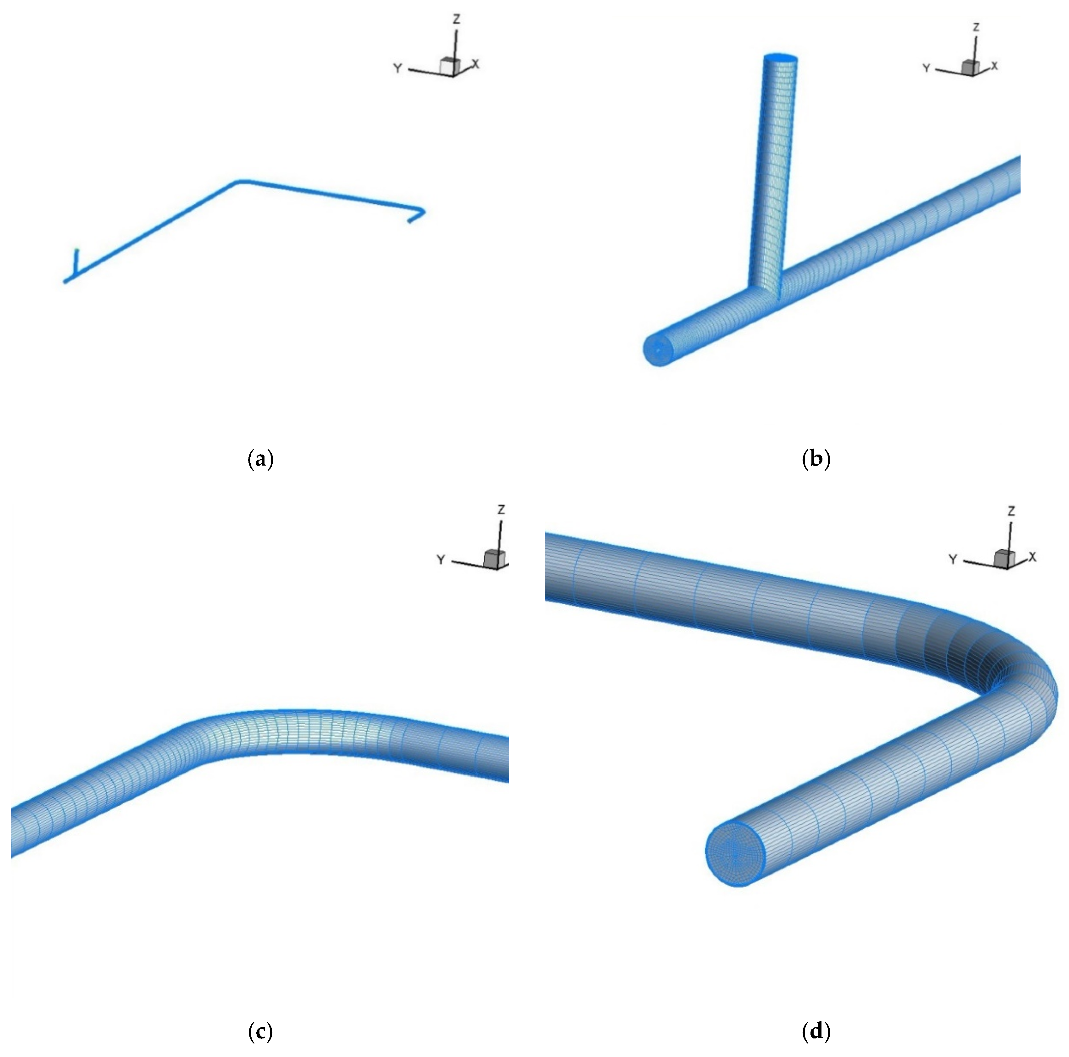
3.2.2. Mesh Generation

Hexahedral mesh can accelerate the calculation speed and reduce errors caused by the angle between the tetrahedral mesh and the flow direction. Therefore, high-quality hexahedral mesh is utilised in this study for calculation speed and accuracy. The inner diameter of the pipe is only 40 mm, while the length of the simulated pipe section is about 8 m. The length-to-fineness ratio reaches 200:1. Since this entity has a large fineness ratio, a Cooper mesh is generated to decompose the complex assembly into a combination of simple assemblies. Pave mesh is generated at boundary layers, and the volume mesh is finally generated after encryption, with a total of 190,000 meshes. The inclination is found to be less than 0.6. The mesh inclination is acceptable when it is less than 0.9, and the mesh quality is acceptable when it is less than 0.7. Figure 3 is the three-dimensional schematic of the generated meshes from different viewpoints.

3.3. Conditions

3.3.1. Parameters and Conditions

According to the optimal combination of settings for two-phase flow flushing in [10], the round nozzle placed at the bottom of the pipe (air inflow time is 4 s and air cut off time is 6 s) is selected for numerical simulation. Since the air–water two phases in the pipe are in an unstable state in one period, the 10 s period is divided into 2 s time units, i.e., they are simulated at six different time points, 0, 2 s, 4 s, 6 s, 8 s and 10 s.

3.3.2. Boundary Conditions

The inlet pressure is set at 0.3 Mpa, which is kept constant by the pressure regulator valve at the outlet of the gasholder. The inlet velocity is set at 2.07 m/s, that is, the water flow velocity in the pipe during single-phase blank test. The outlet of the simulated pipe section (the third pressure test point) is set as the pressure outlet. The pressure data of one period is fitted into a polynomial function, which is brought into the UDF and calculated by an unsteady solver.

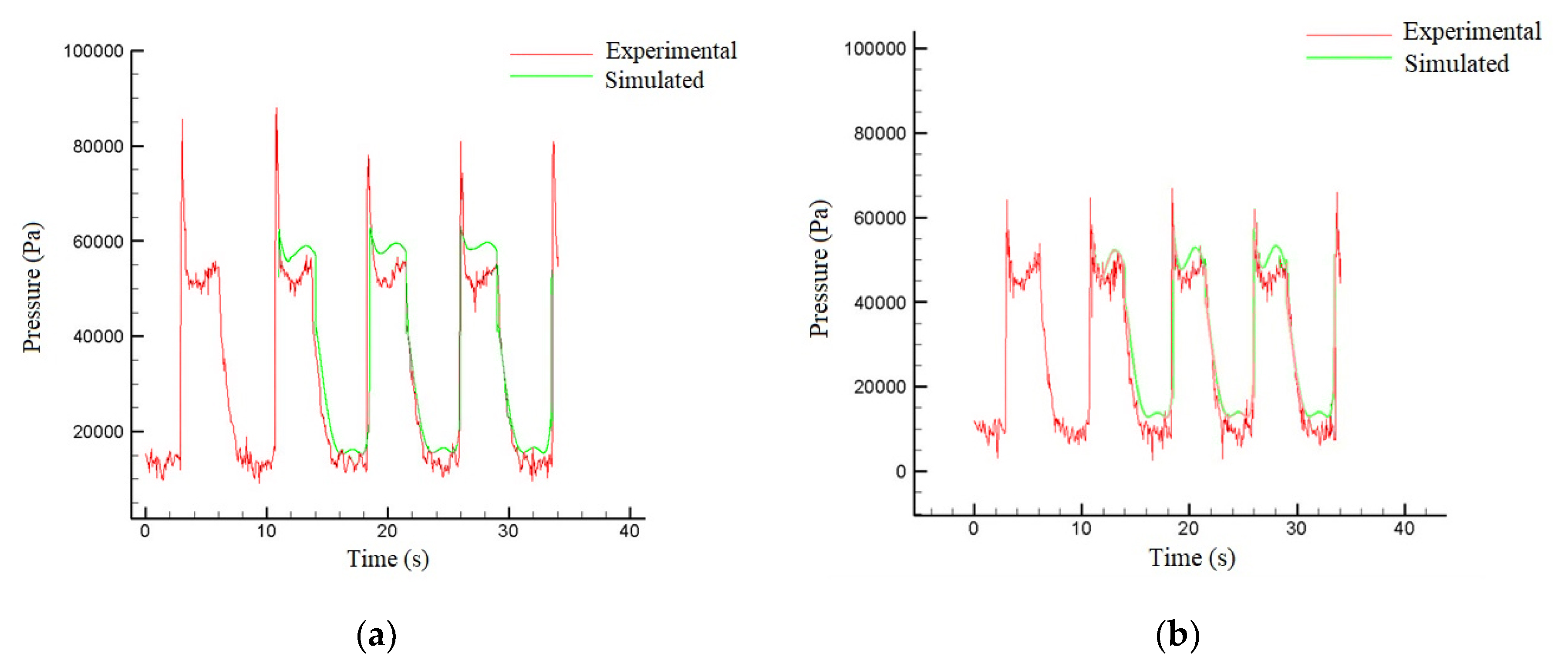
3.4. Model Verification

Figure 4 shows the simulated results compared with the experimental results at the first and second pressure test points in one period.

From Figure 4, the plot of simulation pressure data are fitted to the shape of the experimental pressure data at the first and second pressure test points, but at pressure peaks they have slight differences. This is because the pressure inside the pipe will have an abrupt change at the time of the air inlet, but during the simulation process, this abrupt change is discontinuous and singular points are formed at the time of the air inlet and, in the above two figures, these singular points are excluded resulting in smooth curves.

3.5. Simulation Results

Simulation of one period is carried out on the working condition of a round nozzle placed at the bottom of the pipe (air inflow time is 4 s and air cut off time is 6 s). The verification shows the plot of simulation pressure data are generally fitted to the shape of the experimental data at the first and second pressure test points. Based on the aforementioned results, the diagram of pressure, water-phase velocity, and water-phase volume radio distributions at different points of time in a period are obtained. Their time interval is 2 s. The simulation results of the shear force variation against time at the first and second pressure test points are also obtained.

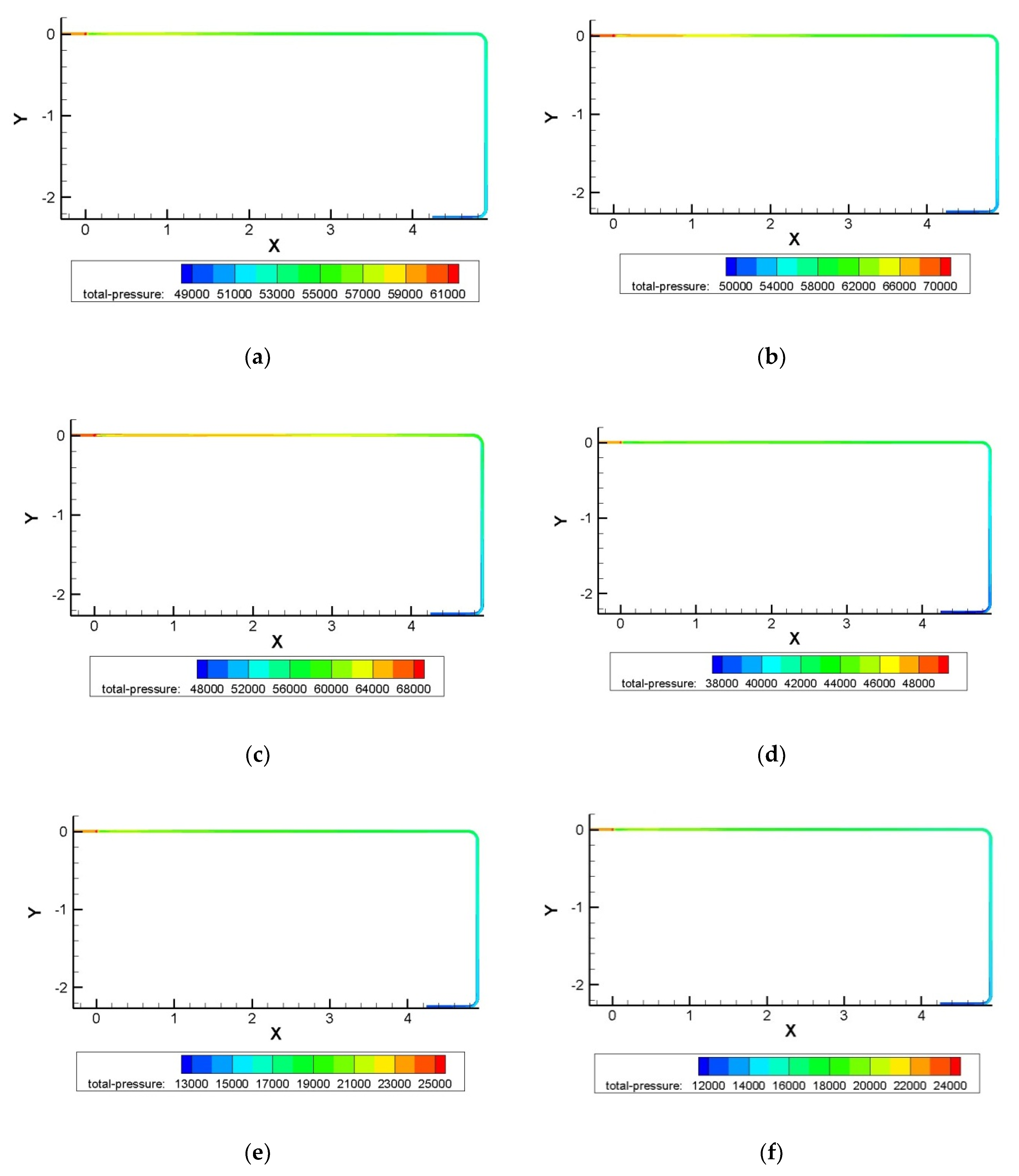
3.5.1. Mapping of the Pressure Distribution

The simulated mesh entity is three-dimensional. The position of water inlet is vertical, while the positions of air inlet and simulated pipe section are horizontal. Therefore, the pressure of the horizontal section of the intercepting pipe is selected. Figure 5 from (a) to (f) shows the trend of pressure against time. Figure 5 is the pressure distribution map of the horizontal plane of the simulated pipe section centre. It shows that within the first 4 s air inflow time, the pressure in the pipe gradually increases along the direction of water flow (the positive direction of the X-axis). After 4 s, the air inflow stops and the pressure in the pipe gradually decreases until the end of the 10 s period. Then the next two-phase flow cleaning period starts.

3.5.2. Mapping of the Water-Phase Velocity Distribution

Figure 6 shows the water-phase velocity distribution map of the horizontal plane of the simulated pipe section centre. It shows that within the first 4 s air inflow time, the water-phase velocity in the pipe gradually increases along the direction of water flow (the positive direction of the X-axis). After 4 s, the air inflow stops and the water-phase velocity in the pipe gradually decreases until the end of the 10 s period. Then the next two-phase flow cleaning period starts.

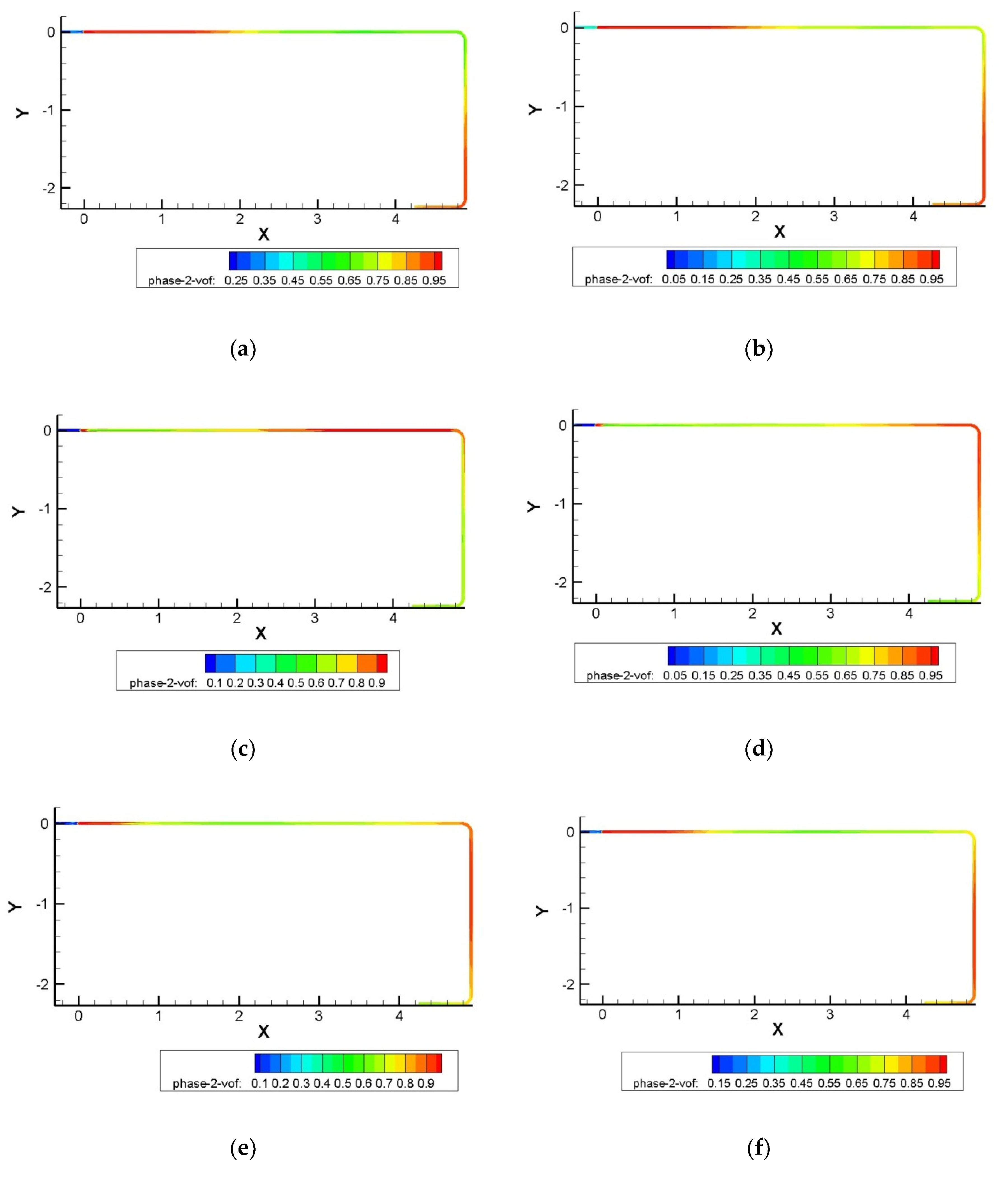
3.5.3. Mapping of the Water-Phase Volume Ratio Distribution

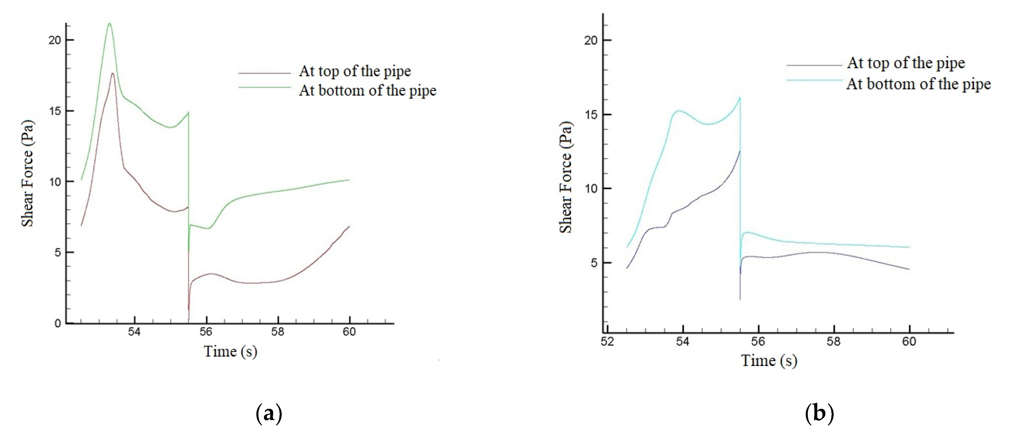
Figure 7 shows the water-phase volume ratio distribution map of the horizontal plane of the simulated pipe section centre. It shows that in one period, water with a slug flow state moves towards the end of the pipe, and this state lasts up to approximately 2 m at its longest, which is basically consistent with the slug flow length observed in the test. This verifies that the air–water two-phase flow flushing process is a slug flow with severe turbulence.

3.5.4. Shear Force

During flushing, the removal of the “growth ring” is mainly affected by the shear force along the direction of water flow. The direction of shear force on the pipe inner wall is consistent with the direction of water flow. Through simulation, the values of the shear force at the top and bottom of the pipe at the first and second pressure test points are obtained, and the diagram of the shear force against time in a period is also obtained and shown in Figure 8.

From Figure 8, the shear force at the top of the pipe is smaller than at the bottom of the pipe. The first pressure test point is close to the air and water inlets, so the shear force change and fluctuation at the first pressure test point is obvious, which forms a crest. However, the shear force of four monitoring points dropped sharply at the time of stopping the air inflow.

The severe fluctuation of the shear force at the tangential direction of the pipe makes the air–water two-phase flow flushing method its unique advantage, which can efficiently clean the water supply pipeline with less water consumption and flushing time.

4. Conclusions

Numerical modelling and simulation study based on the experimental results are carried out by FLUENT to evaluate the performance of two-phase flow flushing method for removal of the “growth ring”. The simulation results match the experimental results. Pressure, water-phase flow velocity and water-phase volume ratio distributions in a section of pipe are simulated and analysed. Within the first 4 s air inflow time, the pressure and water-phase velocity in the pipe gradually increase along the direction of water flow (the positive direction of the X-axis). After 4 s, the air inflow stops and the pressure and water-phase velocity in the pipe gradually decreases until the end of the 10 s period. The air–water two-phase flow flushing process is a slug flow with severe turbulence. The shear force against time in a period is obtained and analysed. There is severe fluctuation of the shear force at the tangential direction of the pipe for efficient removal of the “growth ring” in the water pipe. This study suggests that elbow pipes cause flushing energy loss, and, therefore, at most one section of elbow pipe is flushed in one flushing period for the best cleaning results. In conclusion, this research establishes a new way to potentially use numerical modelling and simulation results to guide pipe engineers to efficiently and effectively flush water distribution pipelines.

References

1. Zhong, D.; He, F.; Ma, W.; Yuan, Y.; Wang, Z. Study on the Inactivation of Pseudomonas sp. and the degradation of trichloroethylene by Fenton-like reaction. Water 2018, 10, 1376. [Google Scholar] [CrossRef] [Green Version]
2. El-Chakhtoura, J.; Prest, E.; Saikaly, P.; van Loosdrecht, M.; Hammes, F.; Vrouwenvelder, H. Dynamics of Bacterial Communities Before and After Distribution in a Full-scale Drinking Water Network. Water Res. 2015, 74, 180–190. [Google Scholar] [CrossRef] [PubMed]
3. Douterelo, I.; Husband, S.; Boxall, J.B. The Bacteriological Composition of Biomass Recovered by Flushing an Operational Drinking Water Distribution System. Water Res. 2014, 54, 100–114. [Google Scholar] [CrossRef] [PubMed] [Green Version]
4. Husband, P.S.; Boxall, J.B. Asset Deterioration and Discoloration in Water Distribution Systems. Water Res. 2011, 45, 113–124. [Google Scholar] [CrossRef] [PubMed]
5. Husband, P.S.; Boxall, J.B. Field Studies of Discoloration in Water Distribution Systems: Model Verification and Practical Implications. J. Environ. Eng. ASCE 2010, 136, 86–94. [Google Scholar] [CrossRef]
6. Zhao, H.B.; Li, X.; Zhao, M. The “Growth-Ring” of the Water Distribution Pipeline. In Hygiene in Water Distribution Pipeline, 1st ed.; China Architecture & Building Press: Beijing, China, 2008. (In Chinese) [Google Scholar]
7. Teng, H.; Guan, Y.T.; Zhu, W.P. Effect of Biofilm on Cast Iron Pipe Corrosion in Drinking Water Distribution System: Corrosion Scales Characterisation and Microbial Community Structure Investigation. Corros. Sci. 2008, 50, 2816–2823. [Google Scholar] [CrossRef]
8. Li, S.; Zhang, X.J. The Growth and Development of the Biological Membrane on the Water Distribution Pipe Wall and their Influence Factors. China Water Wastewater 2003, 19, 49–52. (In Chinese) [Google Scholar]
9. Wang, T.; Liu, H.; Wei, H.; Ge, W. Numerical Simulation of Two-phase Flow in the Pipeline Cleaning used Barometric Pulse Method. In Proceedings of the 2011 International Symposium on Water Resource and Environmental Protection, Xi’an, China, 20–22 May 2011; pp. 3131–3135. [Google Scholar]
10. Tang, Z.; Wu, W.; Han, X.; Zhao, M. An Experimental Study of Two-Phase Pulse Flushing Technology in Water Distribution Systems. Water 2017, 9, 927. [Google Scholar] [CrossRef] [Green Version]
11. Coronado-Hernández, O.E.; Fuertes-Miquel, V.S.; Besharat, M.; Ramos, H.M. Experimental and Numerical Analysis of a Water Emptying Pipeline Using Different Air Valves. Water 2017, 9, 98. [Google Scholar] [CrossRef]
12. Coronado-Hernández, O.E.; Fuertes-Miquel, V.S.; Angulo-Hernández, F.N. Emptying Operation of Water Supply Networks. Water 2018, 10, 22. [Google Scholar] [CrossRef] [Green Version]
13. Fuertes-Miquel, V.S.; Coronado-Hernández, O.E.; Iglesias-Rey, P.L.; Mora-Meliá, D. Transient Phenomena During the Emptying Process of a Single Pipe with Water-Air Interaction. J. Hydraul. Res. 2019, 57, 318–326. [Google Scholar] [CrossRef]
14. Coronado-Hernández, O.E.; Fuertes-Miquel, V.S.; Besharat, M.; Ramos, H.M. Subatmospheric Pressure in a Water Draining Pipeline with an Air Pocket. Urban Water J. 2018, 15, 346–352. [Google Scholar] [CrossRef]
15. Coronado-Hernández, O.E.; Fuertes-Miquel, V.S.; Iglesias-Rey, P.L.; Martínez-Solano, F.J. Rigid Water Column Model for Simulating the Emptying Process in a Pipeline Using Pressurized Air. J. Hydraul. Eng. 2018, 144, 06018004. [Google Scholar] [CrossRef]
16. Besharat, M.; Coronado-Hernández, O.E.; Fuertes-Miquel, V.S.; Viseu, M.T.; Ramos, H.M. Backflow Air and Pressure Analysis in Emptying a Pipeline Containing an Entrapped Air Pocket. Urban Water J. 2018, 15, 769–779. [Google Scholar] [CrossRef]
17. Coronado-Hernández, Ó.E.; Besharat, M.; Fuertes-Miquel, V.S.; Ramos, H.M. Effect of a Commercial Air Valve on the Rapid Filling of a Single Pipeline: A Numerical and Experimental Analysis. Water 2019, 11, 1814. [Google Scholar] [CrossRef] [Green Version]
18. Besharat, M.; Dadfar, A.; Viseu, M.T.; Brunone, B.; Ramos, H.M. Transient-Flow Induced Compressed Air Energy Storage (TI-CAES) System towards New Energy Concept. Water 2020, 12, 601. [Google Scholar] [CrossRef] [Green Version]
19. Besharat, M.; Coronado-Hernández, O.E.; Fuertes-Miquel, V.S.; Viseu, M.T.; Ramos, H.M. Computational fluid dynamics for sub-atmospheric pressure analysis in pipe drainage. J. Hydraul. Res. 2020, 58, 553–565. [Google Scholar] [CrossRef]
Figure 1. Experimental setup: (1) water tank; (2) water pump; (3) air compressor; (4) gasholder; (5) valve; (6) pulse generator; (7) pressure transmitter; (8) flow meter; (9) computer; and (10) data acquisition module.
Water 12 02470 g001
Figure 2. The photo of experimental setup in the laboratory.
Water 12 02470 g002
Figure 3. The three-dimensional schematic of the generated meshes from different viewpoints: (a) the entire simulated pipe section; (b) the air inlet and water inlet; (c) the elbow pipe; (d) the outlet.
Water 12 02470 g003
Figure 4. The comparison between the simulated and experimental results at the first and second pressure test points in one period: (a) the first pressure test point; (b) the second pressure test point.
Water 12 02470 g004
Figure 5. The pressure distribution of the horizontal axis intersecting surface within a period: (a) t = 0; (b) t = 2 s; (c) t = 4 s; (d) t = 6 s; (e) t = 8 s; (f) t = 10 s.
Water 12 02470 g005
Figure 6. The water-phase velocity distribution of horizontal axis intersecting surface within a period: (a) t = 0; (b) t = 2 s; (c) t = 4 s; (d) t = 6 s; (e) t = 8 s; (f) t = 10 s.
Water 12 02470 g006
Figure 7. The water-phase volume ratio distribution of horizontal axis intersecting surface within a period: (a) t = 0; (b) t = 2 s; (c) t = 4 s; (d) t = 6 s; (e) t = 8 s; (f) t = 10 s.
Water 12 02470 g007
Figure 8. The shear force at the top and bottom of the pipe at the first and second pressure test points: (a) the first pressure test point; (b) the second pressure test point.
Water 12 02470 g008