Quantification of Neonicotinoid Pesticides in Six Cultivable Fish Species from the River Owena in Nigeria and a Template for Food Safety Assessment

Abstract

The Owena River Basin in Nigeria is an area of agricultural importance for the production of cocoa. To optimise crop yield, the cocoa trees require spraying with neonicotinoid insecticides (Imidacloprid, Thiacloprid Acetamiprid and Thiamethoxam). It is proposed that rainwater runoff from the treated area may pollute the Owena River and that these pesticides may thereby enter the human food chain via six species of fish (Clarias gariepinus, Clarias anguillaris, Sarotherodon galilaeus, Parachanna obscura, Oreochromis niloticus and Gymnarchus niloticus) which are cultured in the river mostly for local consumption. This work aims to establish a working method to quantify the likely levels of the insecticides in the six species of fish, firstly by undertaking a laboratory-based study employing the QuEChERS method to extract the four neonicotinoids from fish purchased in marketplace in the UK, spiked with known quantities of the pesticide and using liquid chromatography coupled with tandem mass spectrometry (LC-MS-MS) as the detection method; secondly, by using these samples to optimise the detection method for very low levels of pesticides, then applying the optimised techniques to the analysis of three of each six species of fish taken from the Owena River. A significant benefit of this combined technique is that only small samples of fish are required. Success with this part of the study showed that very low concentrations of the insecticides could be detected in fish muscle. The third aim is to apply a simple quantitative risk assessment model using the data sets obtained, together with information about daily diet, human body weight and recommended safety limits of pesticides in food to illustrate how human health may be affected by the consumption of these fish. The multiple determinations of neonicotinoids in edible fishes in Nigeria are pioneer research and fill a gap in addressing the relationship between waterborne pesticides and food quality in the country. Fundamentally, this work is an exercise to demonstrate the applicability of the aforementioned instrumental method of analysis to fish muscle, which requires only a small sample size of fish; a large number of fish is not required for a proof of concept, in this case. Although not a monitoring programme for the whole Owena River Basin ecosystem per se, this work successfully demonstrates the technical feasibility of a system of chemical analysis and establishes the foundation for ecological surveys in the immediate future. Parameters involving exposures to xenobiotics in ecotoxicological modelling can now be expressed in terms of both mass and molar concentrations of a chemical in animal tissues if so desired.

1. Introduction

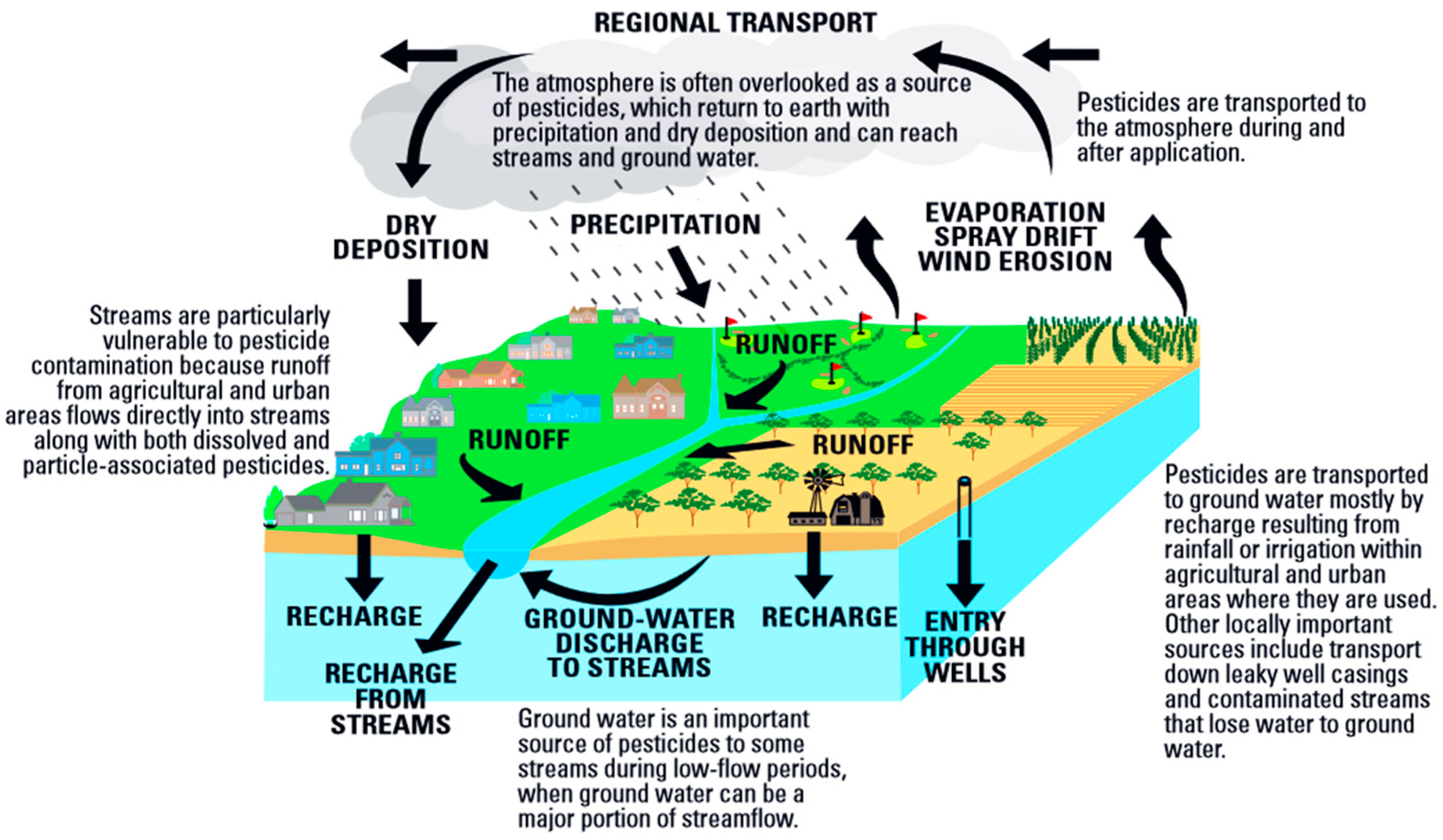
1.1. Neonicotinoid Insecticides as Potential Water Pollutants and Food Contaminants

The cocoa trade is important to the national economy of Nigeria. In 2019, the country was ranked the fourth largest exporter of cocoa products in the world, with fermented cocoa beans being the second most important cash crop [1,2]. The Owena River runs along the major cocoa-producing areas of Ondo State in Nigeria where neonicotinoid insecticides (hereafter called “neonics”) are sprayed onto Theobroma cacao L. (cocoa trees) to control pests such as mirids, a major problem facing farmers. However, when sprayed in plantations, no more than 10% of applied pesticides are taken up by plants, at least 50% end up in soil and up to 30% enter into the atmosphere as vapours and spray droplets, according to estimates/research undertaken by the U.S. EPA [3]. The drift of airborne pesticides into rural and urban populations has also become a public health issue recently [4,5,6]. Globally, the tug-of-war between the reduction of pesticide use and the need to satisfy food demands (and therefore the application of more pesticides) still exists, and national governments struggle to keep that balance—one example being France [7].

Pesticides can also be transported into natural bodies of water such as rivers and groundwater; for example, insecticides from a corn field may end up in a nearby stream due to runoff, or they can seep into groundwater by leaching [8]. The fallout from airborne pesticides can also contribute to this pollution. These transport phenomena do not occur independently of each other but are intimately linked in a cyclic network of processes observed and proposed by Majewski and Capel [9], based on the U.S. Geological Survey and depicted in Figure 1 [10].

Neonics are soluble in water and can be transported long distances by waterways, polluting aquatic ecosystems [11]. It has been suspected that pesticides which enter a river system can cause public health problems. For example, if a river is the main source of drinking/cooking water and if water treatment facilities fail to reduce hazardous substances substantially or remove them completely, it is unsanitary and harmful to the population. By the end of the last century, agriculturalists accumulated so much knowledge about the problem of the pollution of natural bodies of water by pesticides that they were able to build sophisticated mathematical models to perform detailed ecological risk assessments [12]. Moreover, pesticides can also enter the human body from fish eaten from the same natural bodies of water [13].

1.2. Aims of the Present Work

This study has three objectives. The first is to detect, identify and quantify neonics that may have accumulated in six cultivable fishes from the Owena River. The second is to use these data sets to undertake a simple calculation to assess the risks associated with the consumption of these fish. Third, to explore and optimise instrumental analysis for very low concentrations of neonics expected in fish flesh using the capability and operational characteristics of QuEChERS coupled with LC-MS-MS to show the ease of extraction and precise determinations. The four neonics examined in this study are Imidacloprid, Acetamiprid, Thiacloprid and Thiamethoxam (Figure 2).

2. Neurophysiology, Solubilities and Photolysis of Neonics

2.1. Insecticidal Properties

Neonic moieties are derivatives of 3-(1-methylpyrrolidin-2-yl)pyridine, the (S)-(-)-nicotine molecule, which occurs naturally in tobacco leaves, and in rotenone from tropical legumes (of the family Leguminosae; also in plants of the Lycopodiaceae, Crassulaceae, Chenopodiaceae and Compositae families). It is the more active of the two nicotine enantiomers, the other being (R)-(+)-nicotine, in IUPAC notation. Indeed, concerns about the toxicity of neonics are not devoid of foundation, since nicotine itself has been utilised as an insecticide sold commercially as nicotine sulfate (C₁₀H₁₄N₂)₂H₂SO₄ [14,15,16,17]. However, as far as toxic properties are concerned, the U.S. EPA treats nicotine and nicotine sulfate to be the same substance essentially (i.e., the sulfate ion remains a spectator ion in biochemical actions), and both are listed as “extremely hazardous substances” based on known adverse health effects [18]. The ban for its use came into effect in the USA in 2014 [19].

Research and development of neonics commenced in the 1980s by Royal Dutch Shell followed by Bayer in the 1990s, in response to pests’ resistance to actions of commercial biocides during that time. Bayer patented the first commercial neonic, Imidacloprid, in 1985. It eliminates and controls locusts, termites, beetles and stink bugs. Other chemical companies soon patented more neonics and together they have been targeting myriad pests [20,21]. Use is made of the water solubility of neonics so that they can act, as originally intended, as “systemic” insecticides, i.e., they can be coated onto crop seeds and transported throughout the plant, albeit some farmers prefer to spread it on foliage. As one example, neonics are effective in killing chewing insects as well as sucking pests such as aphids. It is necessary to control aphids on sugar beet so that the spread of beet yellow virus is mitigated. Additionally, relative to older insecticides, neonics are less harmful to vertebrates due to their enhanced selectivity to synaptic receptors in insects’ brains. Neonic moieties attach themselves firmly to nicotinic acetylcholinesterase receptors [22] and are not easily dislodged by enzymes, thereby causing overstimulation of the nerve cells, resulting in the paralysis of insects.

Neonics are scrutinised intensely for their effect on bees, which are non-target organisms [23]. Cornell University [24] summarised its review of such effects, clarifying much confusion in the current bee genre. Further, Bayer’s prerogative to attribute bee deaths to varroa mites instead of neonics also needs to be recognised [25]. It must be noted that neonics remain popular insecticides among farmers worldwide to this day. In January 2020, the U.S. EPA allowed five neonics to stay on the market, namely Imidacloprid, Acetamiprid, Thiamethoxam, Clothianidin and Dinotefuran, with recommendations for prudential use [26]. In January 2020, Canada announced plans to adopt new measures to protect pollinators and aquatic organisms but has not indicated the wholesale phasing-out of neonics [27] the way the European Union had in 2018.

2.2. Water Solubilities

Data on the water solubilities of neonics expressed in both mass and molar concentrations, and on their rate of photolysis in aqueous solution, are extracted and calculated from Bonmatin et al. [28] and listed in

Table 1. Solubilities and photolytic rate of neonics in water (adapted and calculated from [28]).

Neonic	Molar Mass (M.W.)	Solubility (ppm), 20 °C, pH = 7	Solubility (mol/dm−3), 20 °C, pH = 7	Direct Photolysis, DT50 (days), pH = 7
Imidacloprid	255.66	610	0.002	0.2
Acetamiprid	222.67	2950	0.013	34
Thiacloprid	252.72	184	0.0007	(recalcitrant)
Thiamethoxam	291.71	4100	0.014	3.7

. With multiple protonable nitrogen atoms on each neonic, (a) to (d) in Figure 2, it is likely that their solubilities are a function of pH, albeit the solubilities in Table 1 being referenced to neutral pH. It is unlikely, however, that the River Owena will ever be saturated with any of these neonics in true solution. Based on the works of Martins [29] and Idu [30], which showed the annual total rainfall on the entire Owena drainage system to be 560 km³, surface run-off was estimated to be 215 km³/year. and distributed among the drainage system. The portion received by the cocoa-growing southwest region was 2.2 × 10¹⁰ m³/year [29,30], or 700 m³ s⁻¹ in S.I. units. The dilution of any solute will be swift and enormous by this substantial volumetric flowrate. A pesticide may never have the opportunity to accumulate to reach its maximum solubility, albeit a finite concentration which is a minute fraction of the saturation value will make its appearance under instrumental analysis. For example, Adegun [31] reported a maximum value of 1.6 × 10⁻⁴ ppm (0.16 ppb) for Thiamethoxam (in the range: 5 × 10⁻⁵ to 1.6 × 10⁻⁴ ppm) in a sample of water from the Owena River. This concentration of Thiamethoxam is a fraction of (1.6 × 10⁻⁴/4100) = 3.9 × 10⁻⁸, which is a mere 1 in 25 million of the saturated value of 4100 ppm (Table 1).

2.3. Photolysis

A significant part of the environmental fate of pesticides is their decomposition by photons. Pesticides which are transported to surface water (at the air/water interface) by means of runoff, wastewater discharge and/or atmospheric fallout are prone to such degradation. The term “DT50” is the time taken for the known (initial) concentration of a chemical moiety to half itself by continuous irradiation by a beam of specified wavelength(s), under strictly controlled experimental conditions. This is called “direct photolysis”. Such is the type of data listed in the last column of Table 1. If the rate of injection of neonics into a river system is mainly due to runoff, then the “sink” terms will be the rates of photolysis, bacterial degradation and oxidation by cytochrome P450 enzymes in organisms. Pesticides in true aqueous solution, adsorption on suspended solids, entrapped in benthic sediments, re-volatisation into the atmosphere and uptake by flora and fauna complete the mass balance.

3. Materials and Methods

3.1. The Study Area

This work is devoted to the detection of neonics in six species of fish of aquacultural interest in Nigeria. The study area was the Owena River at the Owena River Basin (Latitude 07°11′52.2″ N, Longitude: 05°01′14.6″ E) in the Ondo East local government area of Ondo State, Southwest Nigeria. The area is a major producer of cocoa. The fish samples (n = 18, 3 for each fish species) were netted from the Owena River.

3.2. Clarification of Two Technical Terms in Literature

In the literature of public health, food science, ecotoxicology and analytical chemistry, the terms “pesticides” and “pesticides residues” are often used interchangeably without distinction, but not necessarily erroneously. The United Nations’ Food and Agricultural Organization (FAO) defines “pesticides residues” as “Any specified substances in food, agricultural commodities, or animal feed resulting from the use of a pesticide. The term includes any derivatives of a pesticide, such as conversion products, metabolites, reaction products and impurities considered to be of toxicological significance. The term includes residues from unknown or unavoidable sources, e.g., environmental, as well as known uses of the chemical [32]”. For the sake of clarity in this work, the term “neonics” refers to the molecules in Figure 2 only. The term “residues” is reserved for “conversion products, metabolites, reaction products and impurities”.

3.3. Laboratory Chemicals, Reagents, Materials

All chemicals used in this work were of reagent grade; the specifications of the Committee on Analytical Reagents of the American Chemical Society are met [33]. Standards of pesticides of Imidacloprid (IMI), Acetamiprid (ACE), Thiacloprid (THA) and Thiamethoxam (THX) as well as HPLC grade methanol, LC/MS grade water and “Super-clean ^Tmenvi-CarbII/PSA” cartridges were provided by Sigma-Aldrich (Gillingham, UK); sterile “millex” filter units (0.22 µm) from Merck Millipore (Darmstadt, Germany); centrifuge tubes (50 mL) from Fisher Scientific (Loughborough, UK); and anhydrous magnesium sulphate, sodium acetate, ammonium formate, formic acid and 3-chloroaniline (98% purity) from Sigma-Aldrich (Gillingham, UK).

Standard stock solutions of the pesticides were made at 1000 ppm, by dissolving 0.0100 g of each of the pure neonic standards in a mixed solvent of methanol and water (1:1, v/v) and diluting to volume in 10 mL volumetric standard flasks. The intermediate standard solutions were made at 5 ppm. The spiking standards and internal standards were prepared from the intermediate standards at the concentrations of 1 and 0.6 ppm, respectively. The calibration standards were prepared at seven different concentrations of 0.001, 0.005, 0.01, 0.05, 0.1, 0.5 and 1 ppm. The prepared standard solutions (stock, intermediate, calibration and internal) were all stored in sealed PTFE containers in a refrigerator at 5 °C, therefore photolysis of the neonics was also avoided.

3.4. Collection and Storage of Spiked and Unspiked Fish Samples

Samples from six fish species that are cultured in Nigeria were collected and analysed. There were three individuals collected for each species (i.e., there were two replicates for each fish species), and therefore the total number of individuals, n, tested for their neonic contents at Kingston University was n = 6 × 3 = 18. The fish were caught by gill nets of 2 mm gauge. At the time of netting, it was not known if any of the fish contained any detectable neonic. The fish skin was removed, and the muscle tissues were dissected from the fish and homogenised with a meat grinder. All fish samples were kept frozen and flown to the UK where extraction and analysis of neonics would take place at Kingston University [34,35].

In a separate exercise, 18 fish at three per species of mackerel, cod, haddock, halibut, tuna and salmon not from Nigeria were purchased from a market close to Kingston University. These fish were spiked with the four neonics to find out the time required to process 18 fish samples, the chemicals and reagents needed to carry out analysis, the services required of laboratory technicians, and refrigeration facilities for fish. All this is done to identify any technical difficulties that might have jeopardised the analysis of the Nigerian fish samples when they arrived in the UK. It was essential to validate whether neonics can be extracted from the fish matrices and estimate the minimum amount of a neonic required in order to elicit a response from the analytical equipment. This was an exercise in experimental design, planning, training and acclimatisation. The results from this validation exercise do not form part of any scientific report or this article.

At the core of the present work is the demonstration of applicability of the aforementioned instrumental method of analysis to fish muscle, and its requirement for only a small sample size of fish. A big shoal of fish is not required for the proof of concept. Although this work is not a monitoring programme for the Owena River Basin ecosystem, it lays the foundation for a pilot-scale surveillance project to be carried out in the near future. Once confidence in the analytical results is established, the same analytical system can be set up in Nigeria where much larger sample sizes can be handled. For this study, it does not matter if the sample mean does not reflect the population mean as it is not intended to represent the fish population of the Owena River, but to demonstrate the practicality of the instrumental method of analysis in the laboratory.

The six species of fish caught from the Owena River Basin are:

• Clarias gariepinus (Burchell, 1822), the African sharptooth catfish; Clariidae (airbreathing catfishes);
• Clarias anguillaris (Linnaeus, 1758), the mudfish; Clariidae (airbreathing catfishes);
• Sarotherodon galilaeus (Linnaeus, 1758), the mango tilapia; Cichlidae (cichlids);
• Parachanna obscura (Günther, 1861), the obscure snakehead fish; Channidae (snakeheads);
• Oreochromis niloticus (Linnaeus, 1758), the Nile tilapia; Cichlidae (cichlids);
• Gymnarchus niloticus (Cuvier, 1829), the African knifefish; Gymnarchidae (abas).

3.5. Extraction of Neonics from Fish Samples

The QuEChERS procedure is a two-stage exercise. Stage 1 is the extraction of the target chemical from the sample matrix, and Stage 2 is what is called the “dispersive solid phase extraction (dSPE)” step to wean unwanted material from the extract which would otherwise interfere with subsequent determination of the chemical species of interest, here by liquid chromatography-tandem mass spectrometry (LC-MS-MS). The dSPE method shows many advantages over its conventional SPE counterpart in terms of the simplicity of the procedure.

• Stage 1: sample extraction.

Analytes were extracted from samples through the addition of an appropriate solvent and a blend of salts [36]. The salts enhance extraction efficiency and induce a phase separation between normally miscible organic solvents and water in the sample. The choice of solvent system is of fundamental importance. In fact, different solvent mixtures, adsorbent type and amount and sample digestion procedures were all evaluated in terms of extraction efficiency and clean-up.

Optimisation of the leaching of neonics from fish meat samples was achieved through the observation of the extraction effectiveness of supposedly “blank” fish meat samples which had been purchased from Kingston Market, then spiked with neonics after. There were three parameters to be optimised:

• Solvent type. Two solvent systems were tested:

  (a)

  Non-aqueous: methanol, hexane and acetonitrile;

  (b)

  Mixed solvent: de-ionised water, methanol, and acetonitrile.

• Composition of solvent system in terms of volumetric ratios between components. Four ratios were tested:

  (a)

  10:10:10;

  (b)

  10:15:5;

  (c)

  5:10:15;

  (d)

  15:5:10.

• Mass concentration of the “spike” itself in the fish meat samples. Three such concentrations were tested:

  (a)

  0.1 ppm;

  (b)

  0.5 ppm;

  (c)

  1.0 ppm.

This identified the optimal set of parameters as the one with the mixed solvent system composed of de-ionised water, methanol and acetonitrile, in the volumetric ratio of 10:10:10 (i.e., 10 mL each to make up a 30 mL solution), with the mass concentration of the spike 0.1 ppm giving the best results.

One gram of each dried fish meat sample was introduced into a 50 mL centrifuge tube, one tube per sample. Each sample was spiked with a 160 µL aliquot which contained mixed standards of Imidacloprid (IMI), Acetaprimid (ACE), Thiacloprid (THA) and Thiamethoxam (THX). Then, 6 g of the salts magnesium sulfate (MgSO₄) and sodium acetate (CH₃COONa) was also added to aid phase separation and therefore enhance recoveries of analytes. The mixed solvents were added to the samples and salts. This multiple component mixture was shaken mechanically, vortexed and treated in an ultrasonic bath (to aid homogenisation and solution) at room temperature for 10 min. The mixture was further shaken with an orbital shaker for 20 min at 200 rpm, and then centrifuged at 4500 rpm at 10 °C for 3 min. From the supernatant fraction, 7 mL of the liquid was transferred to a 15 mL centrifuge tube and an extra portion of 1 mg of MgSO₄ was added for the removal of excess water from the extracts. Extracts were centrifuged at 4000 rpm at 10 °C for 3 min. The extract supernatants were collected in triplicates and combined for the next stage of the sample preparative procedure, that of clean-up by dSPE. (This was performed at different concentrations of 0.1, 0.5 and 1.0 ppm. The spiking with the best recovery, 0.1 ppm, was used for the analysis of the 18 Owena fish muscle samples).

• Stage 2: dSPE clean-up.

Subsamples of the solvent extracts from Stage 1 were cleaned by dSPE, prior to determination by LC-MS-MS. First, a commercially available SPE cartridge designed for the clean-up of QuEChERS extracts was used. The cartridge’s brand name was “Superclean ^Tmenvi-CarbII/PSA” (Sigma-Aldrich). It was conditioned with 6 mL of acetonitrile before use. The aliquot of extract was transferred into it and interferences such as co-extractives including sugars and fatty acids were washed away from the sample matrix. The base adsorbent was constituted of primary and secondary amines (PSA) through which exchange of materials took place during clean-up. Excess water and unwanted contaminants were also removed. The eluents were collected, and the cartridge was rinsed with de-ionised water, 5 mL of acetonitrile and then by water again. A stream of nitrogen gas then dried the cartridge. The extract was reconstituted to a volume of 0.75 mL (750 µL) followed by its filtration (by 0.22 µm membrane), and then transferred to a 1.5 mL amber-coloured vial. A volume of 45 mL of the 0.6 ppm internal standard (3-chloroaniline) was added to the re-constituted clean extracts, vortexed for a minute and analysed by LC-MS-MS.

3.6. Liquid Chromatography-Tandem Mass Spectrometry (LC-MS-MS) Operational Conditions

Separation of neonics by high-performance liquid chromatography (HPLC) was carried out by the “Agilent Technologies 1260 Infinity” system, equipped with an Agilent 5973 network mass spectrometer, for determination (Santa Clara, California, USA) [37,38]. The column has a C18 packing of 5 μm particle size; the column dimensions are 2.1 mm (internal diameter), and 150 mm long. The temperature of the column was maintained at 31.95 °C and each individual injection volume was 10 μL. The auto sampler temperature was set at 10 °C. The washing-up liquid was an equivolumetric mixture of methanol and LC/MS grade water. The elution gradient applied was “50% aqueous, 50% organic”. The phase labeled “mobile phase A” was an aqueous solution of 0.1 wt.% NH₄⁺(HCOO)⁻ and 0.1 wt.% HCOO⁻H⁺. “Mobile phase B” was the organic phase with CH₃OH as solvent, in which 0.1 wt.% NH₄⁺(HCOO)⁻ and 0.1 wt.% HCOO⁻H⁺ were dissolved, and they were employed at 0.27 mL/min. (270 μL/min.) with a total run time of 15 min.

In the Agilent set-up, in-built Jet Stream Technology desolvates (removes the solvent which is aqueous, organic or a mixed sovent) the analyte from the solvent matrix and furnishes analyte concomitantly by means of an electrospray ion source, thereby enhancing sensitivity of the system.

The working parameters that were optimised are as follows. Nitrogen from a cylinder was employed as a “nebulising gas” to produce assemblages of electrically charged droplets which strip the ionised sample of the solvent. The nozzle voltage of the electrospray nebuliser was set at 4500 volts and the jet exits the nozzle at near-sonic velocity, generating analyte ions and dewatering them simultaneously. The introduction of a collinear and concentric “super-heated sheath gas (nitrogen)” to the inlet assembly “significantly improves ion drying from the electrospray plume and leads to increased mass spectrometry signal-to-noise [ratio] allowing the triple quadruple to surpass the femtogram limit of detection” (per verbatim, [39]).

The rate of heat transfer from the “super-heated sheath gas (nitrogen)” to the nebuliser spray is proportional to the temperature difference between the sheath gas and the spray. The temperature of the sheath nitrogen was optimised at 420 °C, and it is this transferred energy which augments both analyte ion production and dewatering. (The sheath gas pressure was set at 45 arbitrary units; an auxiliary gas at 50 such units). This creates a high ion density in front of the capillary, and in turn translates to higher MS and MS-MS signal intensities and signal-to-noise ratios, thus the birth of the jargon term “brighter signals” amongst practioners.

The dewatered analyte ions then enter the MS through a “resistive and inert” capillary transfer tube that facilitates ion transport [40]. Vestigial remnants of H₂O/solvent molecules are removed by a heated gas which surrounds the capillary tube, set at a working temperature of 200 °C. The collision gas chosen to cause fragmentation was argon and delivered at 1.2 mTorr. The chromatographic acquisition run was programmed in selected reaction monitoring (SRM) mode. The neonic analytes and the internal standards were detected under MS/MS conditions.

The time for the elution of the four neonics was within 15 min. The injected volume was 10 µL of liquid. The characterisation of the masses was performed by the infusion of each of the four neonics after several injections [41]. Mass scan was performed in positive mode with electrospray ionisation (ESI). The collision energy was tuned for better fragmentation between masses = 8 to 42 and the ions were well fragmented, with both precursor and product ions as shown in

Table 2. Multiple reaction parameters for the developed LC/MS/MS method. (IMI = Imidacloprid; THA = Thiacloprid; ACE = Acetamiprid; THX = Thiamethoxam; and 3-CA = 3-chloroaniline).

Neonics	Precursor Ion Masses	MS 1 Resolution (Quadrupole)	Product Ions Masses	MS 2 Resolution (Quadrupole)	Dwell Time (10−3 s)	Fragmentor Masses	Collision Energy (eV)	Cell Accelerator Voltage (V)	Polarity
IMI	256.1	Unit	209	Unit	100	96	14	7	+ ve
	256.1	Unit	175.1	Unit	100	96	18	7	+ ve
THA	253	Unit	126	Unit	100	103	22	7	+ ve
	253	Unit	90	Unit	100	103	42	7	+ ve
ACE	223.1	Unit	126	Unit	100	103	18	7	+ ve
	223.1	Unit	90.1	Unit	100	103	38	7	+ ve
THX	292	Unit	211.1	Unit	100	103	8	7	+ve
	292	Unit	131	Unit	100	104	20	7	+ve
3-CA	128	Unit	92.1	Unit	100	96	25	7	+ ve

Note: The tandem mass spectrometer works in positive polarity, i.e., all ions produced are cations. “Unit resolution” means that one can separate each mass from the next integer mass; i.e., it is possible to distinguish mass 50 from mass 51, or mass 1000 from mass 1001. This definition is commonly used when discussing resolution on quadrupole and ion trap mass spectrometers.

. The precursor and product ions were used for the quantification and confirmation of the analytes [41,42]. The multiple reaction monitoring parameters (MRM) were in agreement with the ones reported by Sugathi et al. [42] in a study on the determination of neonic residues in sugar cane juice. The total ion chromatogram of the four neonic compounds is shown in Figure 3.

3.7. Operational Requirements: Linearity, LOD/LOQ and Extent of Analyte Recovery

To establish the technical suitability of any system of an instrumental method of analysis for its intended purpose is a categorical imperative in scientific inquiry. In this instance, four such parameters are deployed as reference criteria.

I.

Linearity. The linearity of a method is its ability to demonstrate responses that are directly proportional to the concentration of a known analyte. The usual format of presentation is one which includes the coefficient of determination, r², the y-intercept, slope of the regression line “m” and the residual sum of the squares in addition to graphical plotting. For a regression line y = mx + c, calculation of the Pearson’s correlation coefficient (r) shall suffice. Statistically speaking, if a “perfect” linear relationship exists between × and y, then r² = 1; however if R² < 0.95, the linearity of the system is questionable and most analysts re-examine the purity of the analyte as the first step of inquiry, bearing in mind that there can be all sorts of issues such as pipetting or even instrumental drift. Often, the coefficient of determination r² is used, and analysts aim for minimal values of r ≥ 0.98 ⇒ r² ≥ 0.9604 as an acceptable standard of performance (see [38] as an example). In this work, linearity was evaluated by using seven different concentrations of each neonic between 0.001 and 1.0 ppm. The calibration curve for each neonic was carried out three times.

II, III.

Limit of Detection (LOD) and Limit of Quantification (LOQ). LOD is defined as the lowest concentration or quantity of a component or substance that can be reliably distinguished with a specific analytical method, but not necessarily quantified, under the stated conditions of the test. LOQ is defined as the lowest concentration of the analyte which can be detected and quantified within defined limits of certainty (i.e., acceptable precision and accuracy) simultaneously, after replicate measurements are made on the blank and known low concentration, under the stated conditions of the test. (Adapted and modified from [43].)

Table 3. Neonics standard solutions linear range, retention time, coefficient of determination, r², limit of detection (LOD), limit of quantification (LOQ) and regression equation. (Neonics are: IMI = Imidacloprid; THA = Thiacloprid; ACE = Acetamiprid; and THX = Thiamethoxam).

Neonics	Retention Time (min)	Coefficient of Determination, r2	LOD (µg/g)	LOQ (µg/g)	Regression Equation y = m(x) + c
IMI	5.909	0.9992	0.002	0.005	y = 1E6(x) + 7317.3
THA	8.379	0.9995	0.0005	0.003	y = 0.39E6(x) + 1683.2
ACE	6.859	0.9994	0.003	0.004	y = 2E6(x) + 8944.8
THX	5.149	0.9985	0.004	0.005	y = 0.25E(x) + 2024.8

Note that 1E6 = 1 × 10⁶ and 2E6 = 1 × 10⁶.

shows the R², LOD and LOQ values in this work. The value of R² exceeded 0.99 for all the neonics standards. The lowest LOD is 0.005 µg/g, and LOQ is 0.003 µg/g, both values reserved for thiocloprid. The entire LOD ranged from 0.0005 to 0.002 μg/g and the entire LOQ level ranged from 0.003 to 0.005 μg/g.

IV.

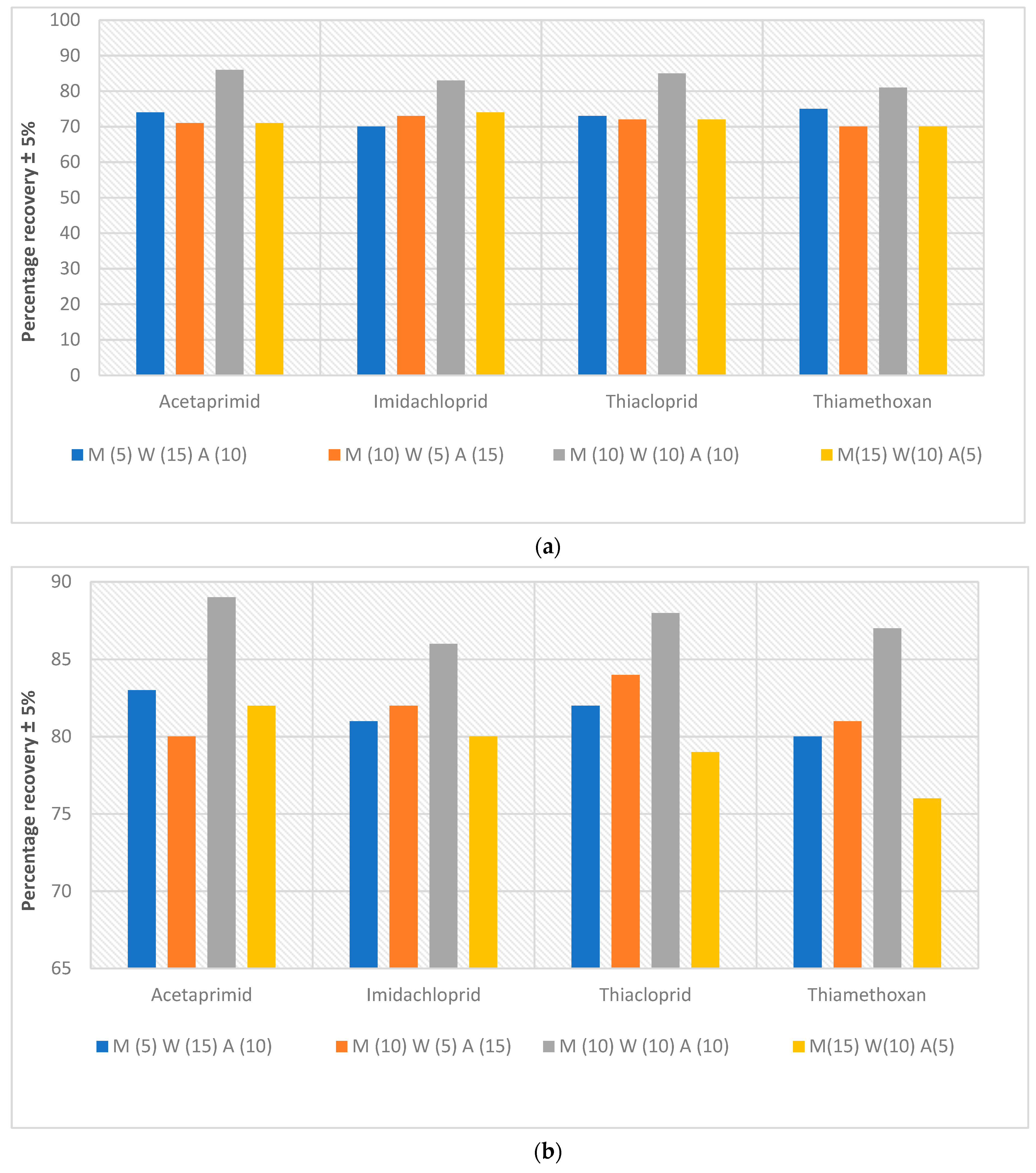
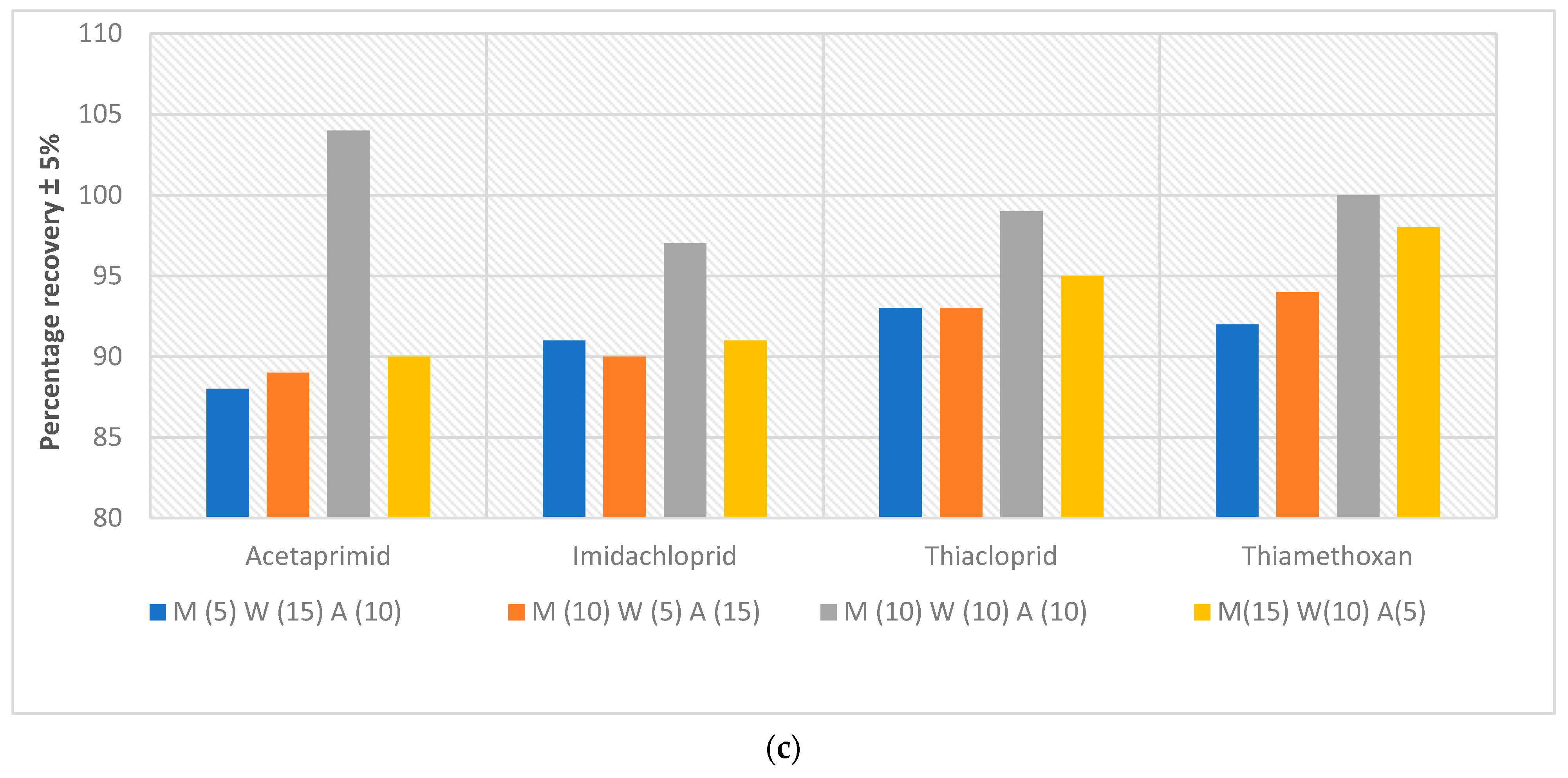
Extent of analyte recovery. Experiments were conducted to discover how much of the neonics that had been spiked into the Kingston market fish can be retrieved from the meat. In these extractive-quantification endeavours, a high % recovery is desired; i.e., a low recovery will lead to gross underestimation of the amount of neonics contained in the Owena fish samples. The recoveries of all the spiked samples were within the range of recommended recovery limits of 70–120% with the coefficient of variation ≤15% between replicates [43]. The recoveries for the fish samples ranged between 70 and 86%, 76 and 89% and 88 and 104% (Figure 4a–c) at 1, 0.5 and 0.1 ppm, respectively. These recovery rates and their reproducibility are acceptable for this work. The recovery results of this study are in agreement with the recovery range reported in a previous study (see [41] (c.f. [42,44])).

4. Results and Discussion

4.1. Biological Data on Fish Collected from the Owena River

With fish, the early stages of development which include the embryonic, larvae, fry and juvenile (fingerlings) are the most vulnerable stages of the life cycle which could be damaged by pesticides. (The other significant water pollutant is the cations of toxic metals such as Cd²⁺ and much has been written about their biological effects.) In this work, the juveniles were caught with nets of 2 mm thick gauge. The names of the six fish species are entered into Column I in

Table 4. Biological data on fish caught from the Owena River.

I	II	III	IV	V	VI	VII	VIII
Fish Species	Range of Lengths (TL)	Range of Weights	Lm (TL at Maturity)	tm (Age at Maturity)	Longevity	Estimated Age	Lower Limit of Kf
Clarias gariepinus (sharptooth catfish)	10–13 cm	40–45 g	30.5–37.5 cm (adults, 90 cm) [45,46]	2 years [47]	6.12 years (up to 15 years [48,49])	<2 years, fingerlings.	1.8 (>1)
Clarias anguillaris (mudfish)	9–12 cm	35–40 g	Male, 14.8 cm Female, 15.7 cm (adults, 65 cm) [50,51,52]	Male, 3.1 years Female, 3.0 years [53]	10–18 years [54]	<3 years, fingerlings.	2.0 (>1)
Sarotherodon galilaeus (mango tilapia)	13–15 cm	60–85 g	18–22 cm (adults, 39.5 cm) [55]	2 years [55]	7 years [55]	<2 years, fingerlings.	1.7 (>1)
Parachanna obscura (snakehead)	14–16 cm	50–70 g	24.5 cm (adults, 45.5–50 cm) [56,57]	2 years (for larger fish) [58]	8–12 years [58,59]	<2 years, fingerlings.	1.2 (>1)
Oreochromis niloticus (Nile tilapia)	13–16 cm	56–72 g	18.6 cm; (adults, 28 cm) [60]	10–12 months [61]	9 years [62]	<10 months, fingerlings.	1.3 (>1)
Gymnarchus niloticus (aba)	15–17 cm	55–74 g	Maximum length observed in adults, 167 cm [63]	At least 6 months [64]	4–14 years (aquarium); up to 40 years (in the wild) [63]	<6 months based on length alone, possibly fingerlings.	1.1 (>1)

. The total lengths (TL) and weights of the fish are listed in Column II and III in Table 4, respectively.

4.1.1. Estimation of Age

The ages of the fish caught are estimated by comparing their measured TL (total lengths) with L_m (the total lengths TL at maturity), at t_m (the time periods taken to reach maturity). The L_m, t_m and longevities of the six fish species are extracted from the literature. For example, in the case of C. gariepinus, the L_m range 30.5–37.5 cm was documented in NAGA (the quarterly publication of the WorldFish Center [45]), with a common length of 90 cm [46]. These data are entered into Column IV in Table 4. The time taken for C. gariepinus to mature, t_m = 2 years [47], is in Column V. The longevity of C. gariepinus in the Mid-Cross floodplain in Nigeria was reported to be 6.12 years [48], shown in Column VI. (A lifespan of 15 years was also claimed [49], but this is likely to be the maximum known). From Column II in Table 4, it can be seen that none of the values of the measured TL of the caught C. gariepinus exceeded the L_m (Column V) documented in the literature, and it can be inferred that their age is less than t_m of 2 years. The deduction is that the collection of C. gariepinus is juveniles, and this is noted in Column VII. The same exercise is repeated for all six fish species.

It is not always possible to find pairs of L_m and t_m readings belonging to the same species in a single publication or database. For example, for C. anguillaris, the value of the mudfish in the Cross River (Nigeria) was L_m = 18−22 cm [50]. The TL of the size of adults was 65 cm, from observation of the fish in West Africa and Lower Guinea (also known as Maritime Guinea, the coastal region of the Republic of Guinea) [51,52]. However, t_m was not recorded, and a literature search revealed that the mudfish in the Sokoto–Rima River Basin (Nigeria) developed to maturity at t_m = 3 years [53] (but the corresponding L_m cannot be readily seen from [54]). The lifespan of C. anguillaris is 10–18 years [54]. The data for S. galileous were extracted from a single FAO report [55]. Meanwhile, the data for P. Obscura and O. niloticus originated from multiple sources [56,57,58,59,60,61,62], as morphological and allometrical data on G. niloticus (aba) are difficult to acquire. Of the aba in Nigeria, Agbugui [62] commented, “There is relatively little research conducted on G. niloticus, its biology and aqua cultural technology have not received extensive study”. However, she mentioned that low fecundity causes “an extended breeding period of 6 months (May to July, and November to January) [which is] a strategy to ensure that the offspring of G. niloticus sufficiently attains the juvenile stage before it is weaned” [62]. This perhaps informs the reader that it takes more than six months for aba to mature, although neither L_m nor t_m was explicitly stated in her paper. By linear interpolation, the length of the aba caught for this work is about 10% of that of the longest aba observed (167 cm, [63]), therefore 10% of a lifespan of 4 years [63] is 4.8 months, which is shorter than the projected time to maturity of at least six months. The three individuals of aba netted were possibly juveniles. Note that the lower longevity of P. obscura was estimated from the Channa argus (Cantor, 1842; the northern snakehead), as their lifespans have been observed to be similar [59]. The data sets in Table 4 are fully referenced. Although the fish are not adults, the assumption of linear growth (lengthening vs. time) throughout the fishes’ life to maturity was implicitly made. Observation of the relationship between age, length and weight of the fishes throughout their life cycles in the Owena River Basin is yet another project.

4.1.2. Condition Factor

In ichthyology and fisheries management, condition is a technical term and a measure of the physical health of a population of fish. Insight into fish condition is attained by comparing the actual weight W of a fish to an expected weight W_e which is a mathematical function of the total length TL of the fish. (The total length TL is the length of a fish measured from the tip of the snout to the tip of the longer lobe of the caudal fin, usually measured with the lobes compressed along the midline. It is a straight-line measure, not measured over the curve of the body.) In other words, condition is indicated by whether the fish weighs more or less than the expected value. The overarching philosophy is that, broadly speaking, if the real weight of a fish exceeds that of its expected weight, then it is deemed “healthy” if not “plumb”. The condition of an entire population is an ensemble average of the health of individuals. During episodes of water pollution, condition is a testimony to the “robustness” of a fish populace, or lack of it.

Thomas Wemyss Fulton [64] (formerly Wemyss Alexander Thomas Fulton, 1855–1929) began exploring the relationship between the weight and length of fish in 1902. In 1904, he also acknowledged that the relationship whereby an increase in weight (W) conformed to the cube of the length (L³) is broadly true [65]. Fulton published these findings in his capacity as superintendent to the Scottish Fishery Board’s scientific investigations. He noticed that the weight–length relationship varied with species, location and season, and that it reflects (1) the nutritional status; (2) the reproductive status and (3) environmental factors. Implicit in these pronouncements was the assumption that fish grow isometrically; i.e., growth occurs at the same rate for all parts of the fish body so that its shape remains the same throughout its development. However, there was no mention of a condition factor in the two Fulton publications cited above [64,65]. Indeed, it was Alexander Meek (1865–1949) who applied an algebraic form of the cubic relationship to plaice, in the form of: W = 0.0067 × L³ (W in ounces, L in inches), in 1903 [66]. (Alexander Meek was a demonstrator/lecturer in the Department of Natural Science at the University of Durham at this time, and became Chair of Zoology and also Director of the Dove Marine Laboratory later on). In 1912, Johnstone [67] attributed a formula (in c.g.s. units) to Professor Sir D’Arcy Wentworth Thompson (who taught Alexander Meek at the University College of Dundee as an undergraduate; degree awarded in 1889). The formula was probably proposed before 1907, prior to the publication of the same formula by Heinke and Henking [68] in that year, who emphasised the changeability in the length–weight relationship according to season and to the spawning. The formula takes the form

K_f = 100 × W × L⁻³

(1)

Note that D’Arcy Thompson [69] did not to publish the first edition of his magnum opus On Growth and Form until 1917. In the present work, the authors choose to denote the condition factor by K_f while retaining Thompson’s original formula embodied in Equation (1), in order to distinguish it from all the various expressions of “K” in the literature which differ from it in expression. Historicity of the minting of the term “Fulton’s Condition Factor” is complex, and in addition, the literature is plagued by erroneous attributions and citations. Fortunately, the situation has been clarified by Nash [70].

Efforts to understand fish biology for more than a century have resulted in the establishment of the allometric model in depicting morphometric relationships in fish. The general allometric equation for the length–weight relationship is of the parabolic form [71]:

W = a.L^b (L > 0)

(2)

The pre-exponential factor “a” is known as the coefficient for body shape. The exponent “b” can only be determined empirically. The value of “a” is of the order 0.1 for small, round fishes, 0.01 for streamline fishes and 0.001 for eel-shaped fishes. The logarithmic form of Equation (2) is

log₁₀(W) = b.log₁₀(L) + log₁₀(a)

(3)

Equation (3) is an equation of a straight line with b as the slope and log₁₀(a) as the intercept (subjected to the condition: when L = 0, W = 0). Note that Equation (2) is a special case of the general Equation (3) in which b = 3, when growth is assumed isometric. However, a fish stock rarely exhibits isometric growth, with the result that K becomes a function of length, so that dK/dL ≠ 0. In Equation (3), if the exponent b > 3, the fish grows faster in weight than in length (this is called positive allometric growth), and when b < 3, the fish grows faster in length than in weight (negative allometric growth).

A value of K_f > 1 is usually interpreted as an indication of good health of a fish assembly while K_f < 1 means otherwise. As an example, the combined sex values of a, b and K_f were determined for C. gariepinus in Lake Naivasha (Kenya) to be: 0.002, 3.232 (b > 3 implies a positive allometric growth pattern) and 0.5527 (i.e., K_f < 1), respectively [72]. The researchers concluded that C. gariepinus showed “an indication of the unhealthy status of the population with less tissue energy reserves, depressed reproductive potential and low survival”. In the Nigerian Institute for Oceanography and Marine Research, C. gariepinus reared in flow-through tanks under experimental conditions fared better, when K_f was computed to be 0.79 (combined sex) [73].

Regardless of the establishment of sophisticated statistical models depicting the growth of fish, Equation (1) remains a popular and powerful tool in monitoring the well-being of fish. For example, the Department of Primary Industries of the State of Victoria (Australia) uses Equation (1) to monitor the progress of the hatchery-produced fishes Salmo trutta (Linnaeus, 1758, the brown trout), Oncorhynchus mykiss (Walbaum, 1792, the rainbow trout) and Oncorhynchus tshawytscha (Walbaum, 1792, the chinook salmon). A bolded capital K instead of K_f is used to denote the same condition factor defined in Equation (1). With the Australian salmonids just mentioned, condition factors fall within the range 0.8 to 2.0. For example, the judgment passed is such that a trout with a score of 0.8 is an “extremely poor fish, resembling a barracouta; big head and narrow, thin body”. However, a trout with a score of 2.0 is in “excellent condition, a trophy class fish”. (Between these top and bottom leagues, there are three more categories of fish condition). Anglers can read off the K-charts covering the weight and length ranges W = 100–4500 g and L = 20–60 cm [74]. Other simple methods for the assessment of tropical fish stocks are available [75].

In principle, if the length and weight of every single individual in a population are known, a simple mathematical technique to determine the least numerical value of K_f of a populace can be obtained by dividing the smallest weight encountered in an individual by the highest value of L³ (i.e., the TL of the longest fish, which may or may not be the same individual; it need not be the same for this theoretical exercise). Here, one is simply dividing the smallest number by the largest in a collection of numbers. If the calculation results in K_f > 1, then a calculation pertaining to the real length and weight of any individual fish will show that the inequality K_f > 1 always holds. K_f can then be interpreted to represent the least favourable condition (e.g., during a vulnerable stage of the lifecycle of the fish). Conversely, if K_f ≤ 1 is the result of dividing the highest W value by the smallest number of L³, then inequality K_f ≤ 1 will hold for all individuals. K_f can then be interpreted to represent the theoretical best condition. Then, it is necessary to investigate what percentages of fish are in the K_f > 1 and in the K_f ≤ 1 categories, and whether this is acceptable for the purpose of fisheries management. If the length–weight data can be obtained from large sample sizes of a fish species, gathered over several lifecycles from different populations in close geographical propinquity, then the lower and upper theoretical boundaries of K_f may also elucidate the ecological limits to which a particular species can be potentially subjected to. This is a new tool worth exploring further for preliminary investigations into fish conditions.

For the sake of illustration alone, and without generalisation to the entire course of the Owena River, the minimal K_f values were calculated for all six fish species in this work using the ranges of values from Columns II and III, resulting in Column VIII in Table 4. For example, for C. gariepinus:

K_f = 100 × (lowest weight) × (highest TL)⁻³ = 100 × 40/13³ = 1.8

(4)

All the K_f values calculated in this fashion are greater than one (K_f > 1) (see Column VIII, Table 4). The fingerlings seem to be in good condition.

4.1.3. Examples of Conditions of Fingerlings in Aquaculture

Values of K_f have been used to monitor the progress of fingerlings in experimental aquariums with a view to gather aquacultural data on the type of feed necessary for optimal growth. Here are a handful of examples.

• C. gariepinus. Feed for fish farming is the most expensive item of all production costs, in the region of 50–70% [76]. It is strongly linked to the fluctuation of global energy prices, but fish farmers have attempted to discover ways to reduce the cost of feed materials. For example, an attempt was made to reduce the cost of feeding sharptooth fingerlings by partially substituting a formulated “Coppens” feed (45 wt.% protein in 2 mm pellets [77]) with Eichhornia crassipes (Mart.) Solms, 1883 (the water hyacinth) [78]. In the control experiment, the fish diet was not substituted with hyacinth, and the corresponding value of K_f at the commencement of the 70-day experiment was 0.6 which increased to 1.02 at the end. When 20% of the Coppens diet was substituted with hyacinth, K_f dropped to 0.96 (a decrease of 5.8%); when 40% of the diet was substituted, K_f dropped even further to 0.85 (a decrease of 16% from the control value of 1.02). The experimenters settled for a 20% substitution and did not compromise quality for the sake of some cost savings.
• C. anguillaris. Whether an aquatic environment happens to be natural or artificial, the transition from larvae to fingerling is always challenging. Successful laviculture depends on a diet of the smallest zooplankton (rotifers) [79], but growing monocultures of freshwater rotifers such as the much-studied Brachionus calyciflorus (Pallas, 1766) have their difficulties and the quest is for viable mixed cultures. In a set of experiments [80], three groups of larvae were fed with a different type of diet each: Diet 1 contained the freshwater rotifer only (the un-enriched diet), Diet 2 contained the same rotifer with cod liver oil added (the enriched diet) and Diet 3 was a mixture of rotifers, copepods and cladocerans (the mixed diet). At the beginning of the experiment, K_f = 0.6 for all three groups of larvae. The values of K_f peaked at t = 5 days simultaneously for the larvae fed with Diet 1 and Diet 2, at 1.3 and 1.8, respectively. Eventually, both of these K_f values fell to just below 1.10 at t = 24 days (end of the observation period). For the larvae on Diet 3, K_f reached a peak much later at t = 15 days with a value of 1.60, which fell to 0.8 at t = 24 days. Larvae fed with the mixed diet also had the lowest survival rate, of just 39%. Therefore, it seems that a diet containing monocultures of rotifers gave the best results and there may be no need to add cod liver oil.
• O. niloticus. The effect of increasing the weight percentage of maltose in a formulated diet of 11 ingredients (which includes maltose) on the growth of Nile tilapia fingerlings has been investigated [81]. The mean condition factor K_f was used to indicate the health of the fish at the end of an eight-week observation period. With no maltose in the control, K_f = 1.64. At 20% maltose, K_f hit a maximum value of 1.86. At maltose concentrations > 20%, K_f decreased; in fact, it dropped to 1.72 at 30% maltose. Overall, the Nile tilapia fingerlings were in good condition throughout the experiment. Occasionally, the growth patterns of the fingerlings of the Nile and mango tilapias are juxtaposed under similar rearing conditions [82]. A deep analysis into the feeding and growth behaviour of the mango tilapia (S. galilaeus) fingerlings also makes interesting reading [83].
• P. obscura. Snakehead fingerlings were fed with three types of diet to discover which affects the best growth [84]. The diets were: (a) live Nile tilapia fry; (b) trash fish (interesting choice of word because if it is a potential resource it may no longer be useless); and (c) compounded feed. After observing growth for 180 days, the best results were furnished by the diet which consisted of live tilapia fry, with the largest gain in weight of 64%, and the largest increase in K_f of 31% (an increment from 0.63 to 0.83). The corresponding survival rate was 84%.
• G. niloticus. From June to November 2018, aba juveniles in Epe Lagoon (Lagos, Nigeria) exhibited very low values of K_f in the range 0.21 ≤ K_f < 0.27. Conservation and management practices for the fish stocks were suggested [85].

4.1.4. Vulnerability of Juvenile and Young Fish

Due to the fact that Imidaclorpid (IMI) was the first neonic to be introduced into the world and is still used in many non-EU countries, its impact on living organisms has the longest history of all the neonics and is the most studied. Here are a handful of cases.

Population Level

Imidacloprid is known to cause decreased viability and hatching success, which suggests that it is more toxic during the earlier developmental phases of fish, even at very low concentrations. Tyor [86] calculated the 48-h L_C50 for the fertilised eggs of Cyprinus carpio (Linnaeus, 1758), the common carp, to be 7.8 × 10⁴ ppb, but for adults, the L_c50s obtained at 3 to 96 h have all been reported to be >1.2 × 10⁵ ppb [87]. At 10% of the L_C50 (7800 ppb) for the fertilised eggs, depreciation of the viability of embryos in eggs was noticeable, decreasing from 92% (control) to 90% [86]. Islam et al. [88] also reported damage at early stages of development: the 48-h L_c50 was 611 ppb for embryos and 2.1 × 10⁴ ppb for larvae. Özdemir et al. [89] studied the acute toxicity on adults of the common carp. They found that histological alterations were induced in the gills and liver of the carp at the two concentrations 1.4 × 10⁵ ppb and 2.8 × 10⁵ ppb (these are much higher than the doses applied to eggs and larvae), after a gradation of time exposures, with most damage done at 96-h exposure. However, the adult brain showed resilience to acute toxicity. Severe lesions had not appeared in the 96-h exposure, demonstrating that that toxicity is organ-specific. All the research work mentioned in this paragraph may suggest that Imidacloprid has the ability to affect various stages of the lifecycle of a fish, in laboratory conditions, at adequately high doses.

Trophic Level

A scenario regarding the impact of Imidacloprid on a food chain is worth mentioning. Together with the insecticide Fipronil, Imidacloprid adversely affects the growth and development of Oryzias latipes (Temminck & Schlegel, 1846), the Japanese rice fish, also known as medaka [90]. It resides in paddy fields, and the young fish feed on insects. When the insect population was reduced by pesticides, the food supply for fish also dwindled. This predator–prey relationship between fish and insect may be significant in our present work. The possibility exists that fish abundance is affected by lack of food rather than direct toxicity of insecticides, including those already ingested by insects.

Gaps in Knowledge

In aquaculture, aeration, water and diet quality, temperature and pH seem to be the main controlling factors for good growth. These are also important parameters in the wild, but it is possible that anthropogenic and arthropogenic pollution, climate change, diseases, a change in predator–prey relationships in trophic levels and invasion by foreign species leading to increased competition for resources can depreciate the well-being of a fish community substantially. The effects of changes in any one of these parameters may cascade throughout aquatic environments and cannot be readily predicted. Eggs, larvae and fingerlings remain the most vulnerable.

4.2. Neonic Content in fish Collected from the Owena River

4.2.1. Determination of Neonics in Fish Muscle

In

Table 5. Mass concentrations of neonics in six fish species (means and range per individual) and estimated daily intakes (EDI), acceptable daily intakes (ADI) and risk assessment for humans. Data on neonic compounds include: Thiacloprid (THA), Acetamiprid (ACE) and Thiamethoxam (THX).

I	II	III	IV	V	VI	VII	VIII
Fish Species	Neonics	Range (µg/g)	Mean ± σ (µg/g)	EDI (µg/kg Body Mass/day)	Maximum ADI (µg/kg Body Mass/Day) [91,92,93,94,95]	Risk Index (EDI/Max. ADI)	Risk Assessment
C. gariepinus	THA	0.08–0.10	0.09 ± 0.07	0.054	10	5.4 × 10−3 < 1	No risk
	ACE	0.04–0.09	0.07 ± 0.05	0.041	70	5.8 × 10−4 < 1	No risk
C. anguillaris	ACE	0.12–0.16	0.14 ± 0.03	0.082	70	1.2 × 10−3 < 1	No risk
	THX	0.05–0.10	0.08 ± 0.02	0.047	80	5.9 × 10−4 < 1	No risk
S. galilaeus	THA	0.02–0.06	0.04 ± 0.01	0.023	10	2.3 × 10−3 < 1	No risk
	THX	0.04–0.09	0.06 ± 0.02	0.035	80	4.4 × 10−4 < 1	No risk
P. obscura	THA	0.02–0.04	0.03 ± 0.01	0.017	10	1.7 × 10−3 < 1	No risk
	ACE	0.01–0.03	0.02 ± 0.01	0.012	70	1.7 × 10−4 < 1	No risk
	THX	0.03–0.05	0.04 ± 0.03	0.023	80	2.8 × 10−4 < 1	No risk
O. niloticus	ACE	0.02–0.08	0.05 ± 0.02	0.029	70	4.1 × 10−4 < 1	No risk
	THX	0.12–0.14	0.12 ± 0.10	0.070	80	8.7 × 10−4 < 1	No risk
G. niloticus	THA	0.06–0.10	0.08 ± 0.05	0.047	10	4.7 × 10−3 < 1	No risk
	ACE	0.02–0.06	0.04 ± 0.03	0.023	70	3.3 × 10−4 < 1	No risk
	THX	0.05–0.09	0.07 ± 0.02	0.041	80	5.1 × 10−4 < 1	No risk

, the mass concentrations of each neonic which has been identified in all fish individuals are determined by mass spectrometry outlined in Section 3. The fish species and neonics are listed in Columns I and II, respectively. Imidacloprid (IMI) was not identified in any of the fish samples. The corresponding range of values of the mass concentrations, in units of µg/g (micrograms of neonic present in one gram of fish muscle), are listed in Column III. The average and standard deviations of the concentrations are listed in Column IV. The data in Columns V to VIII are used to calculate the risks to human health by consuming hypothetical adult fish with identical neonic contents to these fingerlings, an exercise to which we shall return to in Section 4.3. Note that the data contained in Table 5 are all expressed in mass concentrations.

The amount of each neonic type in each fish species can be converted from its mass concentration and expressed in the unit of the nanomole per gram, nmol/g (1 nmol = 1 × 10⁻⁹ mol). For example, for Thiacloprid (THA) with molecular weight = 252.72, its presence of 0.09 µg per gram of C. Gariepinus muscle meat translates to 0.09/252.72 = 3.56 × 10⁻⁴ µmol/g (~0.36 nmol/g). In similar fashion,

Table 6. Amount of neonics determined in the six Owena River fish species: Thiacloprid (THA), Acetamiprid (ACE) and Thiamethoxam (THX).

Fish Species	Neonics	Molar Concentration Mean ± σ (nmol/g)
C. gariepinus	THA	0.36 ± 0.29
	ACE	0.31 ± 0.22
C. anguillaris	ACE	0.63 ± 0.13
	THX	0.27 ± 0.07
S. galilaeus	THA	0.16 ± 0.04
	THX	0.21 ± 0.07
P. obscura	THA	0.12 ± 0.04
	ACE	0.09 ± 0.04
	THX	0.14 ± 0.10
O. niloticus	ACE	0.22 ± 0.09
	THX	0.41 ± 0.34
G. niloticus	THA	0.32 ± 0.20
	ACE	0.18 ± 0.13
	THX	0.24 ± 0.07

can be compiled. The relative abundances in mol% in each fish can also be calculated. Let “A” be any neonic examined in this work, therefore:

Mol % of Neonic A = nmol of A/(amount of all neonic molecules, nmol) × 100%

(5)

Henceforth, Figure 5 is compiled. It is no more than just a snapshot of a moment in time in the lives of 18 fingerlings of the 6 species. As the fingerlings are netted in the same location, they will be swimming in the same stretch of water, eating the same types of insects and/or plankton which may contain the neonics once applied in cocoa farms, encountering the same detritus (which may form part of their diet), and scouring benthic sediments in propinquity.

However, only empirical experimentation can distinguish the differential propensity for each fish species to retain neonics. Fresh fingerlings from eggs hatched in clean water in a laboratory (i.e., not caught from a river) can be reared in tanks with the neonics of interest added. For example, there can be 6 tanks (for 6 species), each holding 20 fingerlings of just one species of fish. The water in the tanks can be dosed with a mixture of the four (equimolar) neonics, at the lowest observed effect concentration (LOEC) of the four neonics; if not, they have to be determined experimentally. LOEC is the “lowest observed effect concentration”. It is the lowest concentration where an adverse effect has been observed in chronic toxicity tests.

The next step is to determine the mass concentrations of neonics in the muscles with the instrumental method presented in this work after a number of days. Under tightly controlled experimental conditions, the distribution of neonics in each fish species is obtained isothermally at preset dissolved oxygen levels and pH values. Repeat the experiment with different dosages of neonics and periods of observation. This will become a set of benchmark data against which data collected in the wild can be referenced. Otherwise, there is no baseline for comparison.

If one does not wish to experiment with live organisms, then one may have to resort to modelling by using data derived from other indicator fishes such as Oncorhynchus mykiss (Walbaum, 1792; the rainbow trout), Lepomis macrochirus (Rafinesque, 1819; the bluegill sunfish) and Pimephales promelas (Rafinesque, 1820; the fathead minnow) used by the U.S. EPA for risk assessments [91], if such data are available from the literature. The implicit assumption (and not often emphasised) is that all fish metabolise a specific xenobiotic at the same rate, a hypothesis which can be put to the test by careful experimentation. Further, models based on octanol-water partition coefficients are available (see [96]), but they are thermodynamic models, not kinetic. In view of the relatively low lipophilicity (high hydrophilicity) of Imidacloprid (IMI) with log₁₀K_ow = 0.57, the Dutch Ministry of Health, Welfare and Sport did not pursue the possibility of a bioconcentration of the neonic in fish, asserting that secondary poisoning is not an issue and a quality standard for water for that effect will not be instituted [97].

The other parameter which cannot be established by a one-stop, snapshot exercise such as the present work is whether the amount of neonics determined in a fish is a steady or unsteady state concentration. If the concentration in any fish organ (e.g., liver or gills) changes with time, unsteady state mass transfer of the potential xenobiotic is said to have occurred. This applies if a pesticide enters a fish body not continuously but intermittently (i.e., in batches), as in the aftermath of feasting on insects (target or non-target, live or dead) which had incorporated neonics through exposure.

4.2.2. Ecotoxicological Models

One of the challenges of ecological modelling is that one does not always suspect the existence of a relationship between a chemical compound and a species, or between species, or between individuals of the same species until food sources, growth, reproduction and survival are threatened. When that happens, modelling rapidly turns ecotoxicological. A lot can be learnt about the natural environment from risk assessments which have been instigated by dangers real and perceived. Fundamentally, the data required for models are the physical, chemical and geological properties of the chemical compound of interest and its toxicity data with respect to the many species of organisms to be protected. Data relevant to specific xenobiotic–organism combinations may or may not be readily available, but institutions and international organisations such as the U.S. EPA and OECD have proposed the most sensitive organisms as indicators of environmental health. For both these organisations, the indicator species for fish are the rainbow trout and the bluegill sunfish [91,98], whose toxicity data may act as a benchmark reference level for other fishes, and prediction of toxic phenomena commences with these data (same approach for crustaceans). The ensuing models are called quantitative structure–activity relationship (QSAR) and interspecies correlation quantitative structure–activity–activity relationship (ISC-QSAAR). The mayfly has also been used as a biological indicator of the well-being of a stream in the Niger Delta (Nigeria), whose abundance has been characterised by the Shannon–Weaver diversity index [99]. Basant et al. [100] commented that work based on these models had focused on a single species and that for a thorough safety inspection of an ecosystem, models should include other species in different trophic levels so that their responses can be assessed, estimated or predicted. (In principle, the authors of the present work tend to agree, but suggest that the single-species application can be reserved for endangered species such as listed bees and exotic birds.) In practice, it is feasible to study only a limited number of species at any one time, in a specific site. A literature search carried out by the authors of the present work has not, so far, identified a single scientific report documenting the risks posed by several neonics, simultaneously, to a community of multi-species fingerlings in the wild.

Nevertheless, the present work has focused on six fish species which can be secondary and/or tertiary (top-level) consumers. To comprehend how neonics ramify and affect an aquatic ecosystem, it is necessary to examine producers, decomposers and detritus first. These include macrophytes, phytoplankton and zooplankton, fungi, bacteria and dead organic matter. The next trophic level to be examined is that of primary consumers. Neonics affect the neurophysiology of aquatic insects and crustaceans greatly, with the mayfly most sensitive to the action of neonics (e.g., the mayfly [99]). Primary consumers also include invertebrates and smaller fish. The presence or absence of benthic macroinvertebrates is a good indicator for the health of a natural body of water. Many fish species make up the group of secondary consumers which can be both predator and prey. Therefore, a food web model can be used to trace the transfer of pesticides through different trophic levels and estimate the exposure level of each animal in the web, but only if it is a mass balance of the xenobiotic in question with respect to time, which means it has to be a rate model. Exposure is only meaningful when expressed in units of absolute mass intake of pesticides per unit mass of animal body, per unit time (a common unit for humans is mg/kg/day). Embedded in the rate data are metabolic rates, including rates of uptake and elimination. One of the difficulties in building a food web model is that most exposures are not reported as tissue or organ concentrations, but with the instrumental method of chemical analysis developed in the present work, it is possible to determine the tissue concentration and thus the dose rate. In addition, risks can be quantified if and only if there are connections between a macroscopic food web model and toxicokinetics, which may mean examining events on the molecular scale.

4.2.3. Cytochrome P450 Enzymes and Chemical Species Specificity

Natural bodies of water contain a myriad of chemical components. While fish have preferred items in their diets, they have no control over the amount of xenobiotics in their aqueous habitats, in their foodstuffs and in sediments. Although earnest efforts are being made to discover whether certain xenobiotics exist in fish, there is no guarantee that all the chemical compounds being sought after will be present in any sample or in any hypothesised combination based on the knowledge of a few parameters.

Moreover, the presence of water contaminants in fish in the wild is not just about their diets in natural habitats, but also about how the internal metabolism of the fish responds to the many physical and chemical agents in their environments. The mixed-function cytochrome P450 monooxygenase system (CYP1A subfamily) is common to all fish and metabolises a large number of exogenous xenobiotics, transforming most of them substantially before excretion. However, as enzymes, cytochromes are highly selective about which reactions they catalyse. Metabolism can lead to detoxification or activation of innocuous molecular entities to toxic intermediates (involving other enzyme systems such as sulfotransferases and acetylases). Use is made of the latter property to control insects. The organophosphorothioate insecticide Malathion is transformed into the toxic metabolite malaoxon by cytochrome P450, but impurities in the commercial product enhanced this toxicity by 10-fold. The damage of O. niloticus (the Nile tilapia) by Malathion was observed by Fahmy [101]. This is called secondary poisoning.

The rates of the enzymic reactions and products (metabolites) vary widely between species (and even between individuals of the same species of fish) and determine the amount of xenobiotic being transformed and ejected per day. It is now understood that many toxicities are caused by metabolites and not by parent compounds. Moreover, P450 enzymes are indispensible in the anabolism and catabolism of endogenous substances such as hormones, steroids, eicosanoids and some vitamins [102]. Perturbation of cytochrome P450 catalysis may have far-reaching consequences for organisms.

Biotransformation of exogenous xenobiotics is sequential. They are classified as Phase I and Phase II reactions. While some exogenous compounds are excreted largely unchanged, oxidases catalyze the incorporation of an oxygen atom, from a molecule of O₂, into the exogenous molecule in Phase I, rendering it more as glucuronic acid (high capacity of conjugation to xenobiotics), sulfate, glutathione or amino acid which renders it less toxic (as larger molecules do not traverse membranes), more hydrophilic and therefore polar. One atom from O₂ becomes an –OH group in the exogenous moiety, the other forms water. The oxidised compound now “fits” into another enzyme and undergoes further transformation in Phase II. It is during Phase I that reactive or toxic metabolites can be produced. In Phase II, the oxidised xenobiotic undergoes another enzyme-catalysed reaction, whereby it is conjugated by an endogenous compound more excretable. Such is the broad commonality in biotransformation between different species of fish. To juxtapose how two fishes metabolise the same pesticide, it may be necessary to extract and isolate the intermediates and metabolites from the uptake of the parent exogenous compound to its excretion.

Some cytochrome P450 enzymes are inducible. Subsequent to exposure of a cell to a particular chemical compound, enzyme activities can increase, sometimes by orders of magnitude. In turn, inducers become substrates for the induced. Detoxification is often enhanced especially when the concentrations of xenobiotics are low to moderate. Variables such as sex, stage of development and water temperature and pH may influence the inductive response. Many enzymes contain a sulfhydryl (-SH) group as part of their active sites, but metallic ions such as Pb²⁺ and Cd²⁺ can form covalent bonds with sulphur atoms, thereby blocking the site and inhibiting enzyme activity irreversibly. In humans, the understanding of drug metabolism, detoxification and lipid peroxidation (which leads to liver cirrhosis) is the result of studying the liver where the concentration of P450 enzymes is the highest (members of subfamilies are also present in the small intestinal mucosal enterocytes and other organs). In fish, detoxification also occurs in the kidney, gastrointestinal (G.I.) track and gills which play a significant role in the absorption, metabolism and excretion of compounds.

A biomarker is a substance in an organism whose presence is indicative of some phenomenon such as disease, infection or environmental exposure. It is an objective measure which captures the state of biological activities at the cytological and/or organism level at the moment of measurement. Biomarkers can therefore provide information on the health of an ecosystem. The phenomenon of cytochrome P450 induction introduced above fits the description. The CYP1As (subfamily) are the most studied biomarkers for this purpose, but other biomarkers have been deployed singly or in conjunction with CYP1As for fish (CYP1A1 for humans). The carcinogenicities of polycyclic aromatic hydrocarbons (PAHs), coplanar polychlorinated biphenyls (PCBs), polychlorinated dibenzofurans and dibenzodioxins have been researched intensely. It is specifically these compounds which induce CYP1A, and that this induction is a lot more sensitive than any other biomarker from the molecular to the population level [103].

Enhanced activity of the three enzymes CYP1A, benzo(α)pyrene hydroxylase and 7-ethoxyresorufin O-deethylase was discovered in Oreochromis Mossambicus (Peters, 1852), the Mozambique tilapia, relative to enzyme activities in fish in an unpolluted stretch of the same river. Since tilapia is known to dwell close to benthic communities, it was suspected that sediments in the river were contaminated with compounds with structures similar to PAH and PCB (and originated from industrial facilities in the vicinity). In the laboratory, it was found that extracts from sediments collected from the polluted stretch of the river did induce the enzymes [104].

An excellent and well-established in vivo biomarker is EROD (ethoxyresorufin-O-deethylase). It is selective to CYP1A activity and induction [105,106,107] and is easy to measure. For example, it has been used to compare the detoxification systems of C. gariepinus and O. nicolitus [108]; see also [109]. Its induction by benzo(α)pyrene has been found to be different in the liver and gills of C. gariepinus [110]. In an environmental impact analysis, O. nicolitus was exposed to an industrial effluent from a textile mill and C. anguillaris to sediment collected from the same river, in order to elicit responses from CYP1A and other biomarkers as indicators of pollution [111]. Other biomarkers to indicate water pollution have been used. For example, Omnia I. El Euony et al. [112] used serum biomarkers to show that 5 ppm of Thiamethoxam (THX) in aqueous solution intoxicated C. gariepinus and also damaged the liver, kidney, spleen and gills histopathologically.

Species specificity in the biotransformation of xenobiotics is evinced in the uniqueness of reaction pathways. Earlier work demonstrated convincingly that O. niloticus (the Nile tilapia) and C. anguillaris (the mudfish) metabolise an exogenous inducer such as β-naphthoflavone differently [113]. The markers assayed were CYP1A proteins, EROD and the post-oxidation enzymes glutathione S-transferase (GST) and UDP-glucuronosyl transferase (UDP-GT). They were determined at Days 3 and 10 of the monitoring period and found to be very different in many aspects. From the results, it became apparent that the timing and extent of induction were also different for each fish. Kinetic data were also obtained. The kinetics of EROD and GST metabolism were related to substrate concentration. The reactions were pseudo-first-order and the Michaelis–Menten rate constant (V_max/K_m) showed that the Nile tilapia is a more efficient catalytic converter of xenobiotics than the mudfish. It was also found that the tilapia tended to excrete metabolites based on glutathione or mercapturic acids, while the mudfish excreted glucuronosyl metabolites. This implies that mechanistic pathways of Phase II reactions of the fishes are different.

As to how differently the fingerlings of the six fish species examined in this work metabolise neonics, the answers to which may explain the relative abundance of the four neonics inside the six fishes, it may be necessary to repeat the experiment described in the last paragraph, but the degree of complexity in the reaction schemes will be greatly increased as one metabolic pathway may couple and/or interfere with another in unexpected ways. However, to be thorough in this investigation, there will be 15 combinations of neonics which need to be tested for each fish species:

(a)

For single neonics, no. of experiments = 4 (i.e., 1 for each neonic);

(b)

For combinations of two neonics, no. of experiments = 4!/{2!(4 − 2)!} = 6;

(c)

For combinations of three neonics, no. of experiments = 4!/{3!(4 − 3)!} = 4;

(d)

For all four neonics present in aqueous solution, no. of experiments = 1.

The number of experiments to be undertaken for one fish = 4 + 6 + 4 + 1 = 15. The number of experiments for all six fish species = 6 × 15 = 90. There are six control experiments, one for each fish species, in which no neonics are added to the rearing tanks. Therefore, the total number of experiments will be 90 + 6 = 96. It is also possible to relate hepatic EROD activity with muscle concentration [114]; the results will be most useful to aquaculturists. Although Imidacloprid (IMI) had not been detected in the small sample of fish fingerlings in this work, its absence leaves a few questions unanswered. Imidacloprid was the first neonic to be registered and used by farmers all over the world, has it all degraded in the environment since? Does it degrade faster than all other neonics? Did the fingerlings excrete IMI quicker than other neonics? Should there be a chemical-specific enquiry for IMI alone? The instrumental method of chemical analysis developed in this work may be useful in the endeavour.

A case of synergism between a pesticide and a pharmaceutical drug has been discovered recently. Schlussel & Leininger [115] showed that Imidacloprid (IMI) and the anti-depressant fluoxetine functioned antagonistically towards each other. Unexpectedly, they caused less harm together than when they were alone with Daphnia magna (Straus, 1820, the water flea, a planktonic crustacean). Therefore, do neonics interact with one another in fishes? The biochemistry is difficult to predict. Successful rearing of fish demands a water source low in contaminants and pre-treatment is often required nonetheless.

4.3. Fish as an Ecological Compartment

4.3.1. Preparative Work for Pilot-Scale Study

In this article, the research work is part of an effort to develop laboratory methods of instrumental analysis and the conceptual tools which will form the foundation of a pilot-scale survey in the immediate area of the same locale where the fingerlings were netted (Latitude 07°11′52.2″ N, Longitude: 05°01′14.6″ E). This preparative work which may enable a preliminary investigation of part of the Owena ecosystem is in progress.

It is useful to look upon the natural environment as consisting of a number of compartments between which mass and energy can be transferred. A compartment can be a homogenous phase such as water, or the biota in water such as fish, or benthic macroinvertebrates. Some compartments are in contact, e.g., air and water at the interface, and therefore a chemical can diffuse from one compartment to another. Sorption of chemical compounds between water and suspended solids/sediments are known processes. An external agent such as rain can wash chemicals in the soil compartment into the lake compartment. The direct input of energy into a compartment can transform the nature of chemical compounds (e.g., photolysis of pesticides in water). Such is the multi-media model that may be used to describe an ecosystem.

To date, precious little is known about how neonics are distributed around cocoa farms in the Owena River Basin in Nigeria or their ecotoxicity. Since the four insecticides Imidacloprid (IMI), Acetamiprid (ACE), Thiacloprid (THA) and Thiamethoxam (THX) may have been used in cocoa farming, the initial step in a risk assessment is to ensure that these neonics are actually present externally of targeted and non-targeted insects (dead or alive). Then, we may be in a position to study their behaviour and map out their fate in the environment, but not before. To meet this immediate challenge, the QuEChERS/LC-MS-MS method of laboratory analysis was developed to identify and quantify more than one pesticide compound, simultaneously, during any one run of the machinery. This method demands an effective procedure for extracting pesticides from different sample materials.

The authors have decided to ascertain the presence of neonics in these four compartments:

• Plantation soil in cocoa farms;
• Surface water of the Owena River;
• Sediments;
• Cultivable fish species (this work).

To indicate an order of magnitude of concentrations in the initial findings, the upper limit of neonic concentrations determined so far in the first three compartments (I to III) are listed in

Table 7. Upper limits of neonic concentrations in compartments of the Owena River Basin.

Ecological Compartment		Sum of Mass Concentrations of all Neonics
I	Plantation soil in cocoa farms	<2000 ppb (i.e., <2 μg/g dried soil)
II	Surface water of Owena River	<0.3 ppb (i.e., <0.3 μg/liter)
III	Sediments	<300 ppb (i.e., <0.3 μg/g dried sediment)

. This will suffice for the purpose of developing the present discourse. The neonics in these compartments were also extracted by QuEChERS and determined by LC-MS-MS. The set of precise numerical values of concentrations will be published in due course, but without the information in Table 7 it would be difficult to put our readers in the whole picture, since fish are in perpetual and intimate contact with both water and sediments, especially the bottom-dwellers/feeders.

Samples from compartments I to III were taken the same time as the fish were netted. After determination for neonics, the first glimpse at their distribution was achieved. This shows that gathering data for a proper monitoring of cocoa farms and their neighbourhoods over two crops seasons (per year) is technically possible.

For the purpose of aquaculture, it will be very helpful to know whether juveniles are contaminated by various pollutants including pesticides, and to which level. The present work focuses on this theme and the results inform us that this can be achieved. The fish compartment can be treated as a subject on its own but can be part of a more comprehensive ecological survey. Regardless of how neonics disperse and distribute themselves in an ecosystem, the neonics content in fish still requires precise determination. This work achieves that end. On a later date, decisions will have to be made whether it is acceptable to rear juveniles in untreated river water. If not, then water treatment facilities have to be installed to produce clean water. To ensure the quality of such water is maintained, it will also require testing for organic and inorganic compounds periodically/continuously. The LC-MS-MS system described in this article will be able to determine vestiges of pesticides and other organic components post-treatment. These data will also complement BOD and COD determinations well.

4.3.2. Diet and Habitat

The constituents of diets and the feeding habits of fish vary with species, stage of development, age, size, season, habitats and all other physical and biogeochemical factors which define an aquatic environment. Here, through literature, an attempt is made to understand the ways in which neonics can enter the fish population by means of examining their microecosystems and dietary compositions.

C. Gariepinus (African sharptooth catfish) is euryphagous, but adults are often quoted as being omnivorous due to the fact that when animal prey becomes scarce, they resort to plants and detritus. The availability of food dictates the kind of diet (and therefore chemical composition). Catfishes are demersal (bottom-feeders) by nature and prey on sluggish benthic organisms (e.g., invertebrates) efficiently, but they certainly prey on fish and filter food at the surface occasionally. At the larval and early juvenile stages, plankton and chironomids (a family of nematoceran flies) are the most important food items. As fingerlings grow in size, the diet diversifies to include other insects and insect parts [116]. It has been reported that early juveniles possess high levels of α-amylase (enzymes for the hydrolysis of starch) and protease (for breaking down proteins) which allows it to consume a variety of foodstuffs [117,118]. Fingerlings certainly need the energy and building blocks to grow. Spawning occurs during the rainy seasons in flooded river deltas, but adults swim towards the inundated plains to breed and return to the river while juveniles remain in the inundated area. During the rainy season, runoff will carry pesticides into rivers more so than the dry season, yet providing another source of neonics. Juveniles return to the river when they are about 1.5 to 2.5 cm. long [119]. The other airbreathing catfish of the same family, namely the mudfish C. anguillaris, is also an omnivore predatory fish whose diet consists of insects and fish. The diet of C. anguillaris juveniles is diverse, “from algae, higher plant material and detritus through larval dipterans [legless flies], rotifers and copepods, to fish” [120].

Much has been written about S. galilaeus (mango tilapia) being a plankton feeder, but earlier work showed that in the stomachs of small individuals 11–21 mm long, copepods and cladocera (water fleas) are abundant with only a small portion of phytoplankton [121]. It has also been reported that fry 1 to 6.9 cm fed on crustaceans, insect larvae and some algae [122]. Fish of lengths 11–15.9 cm (into which the mango tilapia caught for this work falls) consumed many algae, namely Spirogyra (green algae), Pithophora (green algae) and Compsopogon (red algae), together with some higher plant remains and sand particles. However, as mango tilapia grows in length (>30 cm), the diet contains a predominant amount of detritus with only a small amount of algae, fish eggs and sand [122]. The mango tilapia is perceived to be in contact with benthic mud constantly. In an aquarium, the fish (>20 cm) scooped up mud with its mouth while ejecting coarse particles and sand through the gills [122]. S. galilaeus can filter food on the water surface such as 15 μm planktonic particles with devices called microbranchiospines [123], and it also feeds on algae at the bottom of ponds. S. galilaeus is not well known for eating live insects but has been labeled as aufwuch-detritus herbivores [124]. (Aufwuchs are the small plants and animals that encrust upon hard substrates such as rocks).

Akin to all Oreochromis species, the male Nile tilapia (O. niloticus) burrows a nest at the bottom of a pond when mating season arrives. Several females courted by the male then spawn in the nest and the male fertilises the eggs. The females then incubate the eggs in their buccal cavities and remain there through the absorption of the yolk sac. Contrary to popular lore, the Nile tilapia is not a bottom-feeder. It usually feeds in mid-water in the wild, and only goes benthic if food becomes scarce. The Nile tilapia is omnivorous and consumes a variety of natural foods including phytoplankton, macrophytes, planktonic and benthic invertebrates, although its main source of nutrition is periphyton, which is a mixture of algae, cyanobacteria and heterotrophic microbes attached to the surfaces of both submerged and protruded objects of many kinds; films of bacteria on detritus can be part of the diet. Adults are not known to be piscivorous, but juveniles do feed on larval fish besides zoobenthos and zooplankton. Unlike the mango tilapia, the Nile tilapia does not filter food out of water. At 6 cm (TL), the fish becomes herbivorous, using its pharyngeal teeth and its gills which secrete a mucous to engulf and enmesh plankton. The mucous is then swallowed. It is not known whether the Nile tilapia eats live insects. (Précis of [125,126,127,128]).

The African obscure snakehead fish (P. obscura) is carnivorous and demersal, living amongst dense marginal flora in muddy floodplains. In fast-moving rivers, they tend to colonise the tranquil areas. Its suprabronchial chamber (accessory respiratory organs) keeps it alive when habitats turn hypoxic, an important phenomenon to keep in mind. Dissolved oxygen is one of the main parameters which determine the nature and rate of chemical and biochemical transformation reactions. As the oxygen content declines, oxidations are gradually replaced by reductions. Reductions can occur across the double bond between two nitrogen atoms (-N=N) and account for the toxicity of azo dyes (which are known to be carcinogenic to humans), or on the –NO₂ (nitro) group. The resulting amino products can be toxic. It would be interesting to find out whether reduction contributes to the prolonged residence time of xenobiotics in living organisms. Sediments can vary widely in their oxygen content, and in intertidal zones, the oxygen content fluctuates according to the tidal cycle. In the wild, P. obscura preys on small fish, invertebrates and insects (plant detritus discovered in the stomach is probably from the guts of preyed fish), but for much of the time it remains dormant amongst thick vegetation. Larvae feed on algae and protozoa subsequent to the formation of the mouth. Early fry consume plankton and crustaceans. As fry grow, they limit themselves to purely animal food: prawns, shrimps, aquatic insects, young fishes and tadpoles. Juveniles also feed on insects, insect larvae, copepods and prawns. (Précis of [129,130,131,132,133,134,135]).

The African knifefish, G. niloticus, can grow up to 5½ feet in the wild. It is carnivorous and known for its aggressive behaviour, even in captivity, to its human handlers. The natural habitat of the aba is not dissimilar to that of the snakehead. They are located in swampy areas where vegetation is thick, and are dormant during the day close to the roots of aquatic plants. They build 1-m diameter floating nests for breeding. In its natural habitat, it feeds indiscriminately on fish, frogs, crustaceans, snails and insects. However, it is the juveniles that show special interest in consuming insect parts, followed by fish parts [87,134]. Information on the early stages of development of the aba is scant.

Speaking generally, of the six fishes encountered in this work, four live/feed close to bottom sediments, namely the two catfishes, the snakehead and the aba. All their juveniles can feed on insects, insect larvae and insect parts. The fingerlings of the Nile tilapia and mango tilapia feed on phytoplankton, but it is uncertain whether they feed on insects (although fry of the mango tilapia feed on insect larvae). All six species can process and eject sand/sediment. For the sake of argument, let us add up the amounts of all neonics in each species using data in Table 6, and compare the readings between the “insect eaters” and “phytoplankton eaters”. The sums of the means (in nanomoles, per gram of muscle meat) for the six fishes are: C. gariepinus (0.36 + 0.31 = 0.67 nmol), C. anguillaris (0.63 + 0.27 = 0.90 nmol), S. galilaeus (0.16 + 0.21 = 0.37 nmol), P. obscura (0.12 + 0.09 = 0.21 nmol), O. niloticus 0.22 + 0.41 = 0.63 nmol) and G. niloticus (0.32 + 0.18 + 0.24 = 0.74 nmol). These molar quantities are divided into two groups, namely the planktonophages [135] (i.e., phytoplanktivores) and insectivores, and plotted in Figure 6. From this single set of data alone based on a small sample size (n = 18), the hypothesis that insectivores will bear higher contents of neonics than planktonophages can perhaps be made. Larger sample sizes are needed to test this hypothesis.

Inorganic and organic matter can be adsorbed and desorbed from suspended solids and benthic sediments and the flux is continuous. It is possible that adsorbed surface materials can be desorbed by gastric juices with a range of pH and enters into solution before uptake into the blood stream. Much is known about how a fish ejects sand from itself, but understanding the leaching of neonics in fish requires more research aided by physical chemistry and solid–liquid leaching models developed in the field of chemical engineering which had seen application in the washing of soil (for the removal of contaminants such as the organic solvent CCl₄), and to extracting oil from cod livers as a commercially available diet supplement [136,137,138,139].

4.4. Illustration of a Risk Assessment of Hypothetical Consumption of Contaminated Fish

Risk assessment is the key scientific foundation of risk analysis and was developed due to the necessity to make decisions to protect the health and well-being of human populations in the midst of scientific uncertainties. Risk assessments are therefore health and safety assessments. Risk assessment of food chemicals, including pesticides, can be generally described as identifying and characterising the hazards of the chemicals and the risks which will be incurred as a result of exposure of humans to these chemicals present over a specified period of time.

Farmers and personnel in the manufacture of pesticides have close encounters with pesticides most of their professional lives and they incur the risk of acute and chronic poisoning. For the general public, pesticide residues intermingled with foodstuffs are the main source of exposure, and the toxicity may also be acute or chronic. The Forest Service of the U.S. Department of Agriculture [139] had provided an example of an acute exposure involving the consumption of contaminated fish. The scenario is based on a hypothetical situation whereby an adult angler consumed fish which had been netted from contaminated water shortly after an accidental spill into a pond; leaks from factories or overturned trucks after collisions can contribute to this situation. In fact, most people who have ever been acutely affected by pesticides had ingested food contaminated by pesticides, including horrific incidents experienced by cocoa farmers in Nigeria [140,141,142]. Although episodes of acute poisoning are relatively rare, they have alerted food hygienists, public health officials and consumers to the hazardous nature of pesticides. Food poisoning is not uncommon amongst members of the public, but a host of food contaminants are ingested daily without symptoms of deleterious effects. (It is the severity of the dose that renders such contaminants poisonous) Chronic effects are more difficult to monitor and predict, but such is the task of epidemiologists. The crux of the matter is whether the magnitude of any risk to the general public is manageable.

In the present work, levels of neonics in the 18 individuals belonging to the 6 African fish species (i.e., 3 individuals per species) were determined. Since all the individuals are fingerlings, the data gathered and processed here are purely for demonstrative purposes to illustrate the entire procedure of the calculation of risk due to daily intake of fish protein. Here, the exercise should be treated as a preliminary template in which the health risks associated with the hypothetical consumption of adult fish contaminated with similar levels of neonics were evaluated.

It has to be emphasised that the authors of this article do not advocate the consumption of fingerlings caught from any natural body of water.

4.4.1. Methodology

This exercise of risk assessment attempts to estimate exposures to neonics due to consumption of fish, a chief source of protein, by adults in Nigeria. The analysis includes:

(a)

An estimation of the daily intake of fish from databases. From a database called FAOSTAT, the Dutch Embassy in Lagos (Nigeria) extracted the first important piece of information for this calculation: fish consumption reached 13.3 kg/person/year in 2017 in Nigeria [143], or 36.4 g/person/day. (Note that the reported value of 13.3 kg is below the world’s average of 20.5 kg for the same year, 2017 [143]; no update of this numerical value of 13.3 kg was given by UN’s FAO between 2013 and 2019. In 1991, the FAO recommended a minimum dietary requirement of 35 g of animal protein/person/day for human health, but also reported that the consumption in Nigeria at the time was only 7 g [144]).

(b)

Experimental data on the amount of neonics in fish obtained in this work.

(c)

Combination of the fish consumption and fish contaminant information, from (a) and (b), for the estimation of daily exposures from consumption.

(d)

Comparison of exposures thus estimated to benchmark values set by international authorities such as the Fish and Agriculture Organization (FAO) of the United Nations (UN) with the aim of the determination of potential public health impacts.

(e)

Three underpinning assumptions:

• Any other type of food in the daily diet of an adult does not contain any pesticide;
• Other types of pesticides other than neonics are absent in the fish examined;
• If two or more neonics are present in an adult human, they do not nullify nor augment each other’s toxicity. Their biochemistry is independent of each other.

(f)

A safety criterion. If just one of the many neonic components exceeds an “acceptable daily intake” (ADI) limit while others do not, then the fish is deemed unsafe to eat.

The conceptual framework underpinning the risk assessment method outlined above, from (a) to (e), is adapted and modified from a systematic protocol proposed by Dougherty et al. [145] for the prediction of chronic effects such as cancer. Their method has been extended to address non-cancerous pathologies including those with pesticides as a causative factor. Contaminants in many types of food in the U.S.A. were reviewed. Feature (f) above is added by the authors of the present work to safeguard the consumer. In the literature, a case whereby Dougherty’s approach was employed as the basis for the examination of pesticide-related ecotoxicology (and implications for public health) of the Tono Reservoir (Navrongo) in Ghana is documented [146].

Essentially, two mathematical equations and one inequality criterion define the risk assessment method. The calculation is based on the feeding habit of one adult in one day. For any pesticide “X”:

M₁ (μg) = Mass of Pesticide “X” ingested = Concentration of Pesticide “X” in fish (μg/g) × (36.4 g of fish consumed)

(6)

Estimated daily intake:

EDI (μg/kg) = Mass of Pesticide “X” ingested/kg of human body mass
= M₁/Ave. wt. of adult = M₁/61.6

(7)

The value of the acceptable daily intake (ADI) of Pesticide “X” is obtained from a source such as the FAO and fully referenced in the Bibliography.

If EDI ≥ ADI, the risk is significant, and the fish must not be eaten. If, however, EDI < ADI, the fish meat can be eaten. The calculation is carried out for each neonic in every individual fish.

4.4.2. Calculation and Results

The details of the calculation, the results and their tabulation (Table 5) are now described. The fish species and neonics are listed in Columns I and II, respectively. The ranges of the mass concentrations of neonics in sample matrices are listed in Column III.

The calculation commences with an estimation of the daily intake of a pesticide. The first set of data entered into Table 5 belongs to S. gariepinus. The mean concentration of Thiacloprid (THA) in this fish is 0.09 µg/g (Column IV). Assuming that this is the only type of fish eaten on any day, then the mass of THA ingested is (0.09 µg/g) × (36.4 g/day) = 3.28 µg/day.

Ovewole et al. [147] reported that the average body masses of Nigerian adult males and females are 63.8 and 58.4 kg, respectively. Assuming the ratio of male to female in the population is close to 1:1, then the average body mass of a Nigerian is (63.8 + 58.4)/2 = 61.1 kg. The mass of THA ingested can be restated as: (3.28 µg/day)/61.1 kg = 0.054 µg/kg body mass/day, in Column V.

The values of the acceptable daily intake (ADI) of Thiacloprid (THA) [92], Acetamiprid (ACE) [93,94] and Thiamethoxam (THX) [95] are respectively: 0.01, 0.07 and 0.08 mg/kg body mass/day. These data are the entries in Column VI.

The risk indices in Column VII are obtained by dividing the EDI by the ADI (i.e., by dividing the numbers in Column V by those in Column VI), thus 0.054/10 = 0.0054 < 1 (the first number entered in Column VII). Therefore, the daily intake is only half of 1% of the maximum acceptable dose, so that the diet, if taken, is deemed safe.

Therefore, the risk assessment returned a “no risk” verdict, shown in Column VIII. Table 5 is completed accordingly using the sample calculation outlined above. To reiterate, in the hypothetical situation where the full 36.4 g of the muscle of a single species of fish is consumed by a person in Nigeria within the time duration of a day, there is no risk to health from neonics.

A comment on the ADI needs to be made. The “acceptable daily intake (ADI)” is an “estimate of the amount of a chemical in food or drinking-water, expressed on a body weight basis that can be ingested daily over a lifetime without appreciable health risk to the consumer. It is derived on the basis of all the known facts at the time of the evaluation”, so declared the World Health Organization in 2009 [148]. Time passed, and the European Union Food Authority updated the ADI values of Acetamiprid (ACE) and Thiamethoxam (THX), lowering them to 0.025 [149] (from FAO’s 0.07) and to 0.026 mg/kg/day [150] (from FAO’s 0.08), respectively. This raises the risk index (i.e., becoming relatively more unsafe) concerning ACE ingestion by a factor of 0.07/0.025 = 2.80. For ACE exposures, C. anguillaris gave the highest risk index, at 1.2 × 10⁻³ (Column VII, Table 5). The risk index can be revised to 2.8 × (1.2 × 10⁻³) = 3.4 × 10⁻³ < 1 (i.e., it is still safe) and the “endorsement” of safety need not be reversed for other fish species. In the case of THX, risk indices involving this neonic are raised by a factor of 0.08/0.026 = 3.10. For THX exposures, the highest numerical value of the risk index was 2.8 × 10⁻⁴, incurred by ingesting P. Obscura (Column VII, Table 5). The risk index can now be revised to 3.1 × (2.8 × 10⁻⁴) = 8.7 × 10⁻³ < 1 (i.e., it is still safe) and, again, implication of safety need not be revised for other fishes. The ADI of THA was not updated by the EU and remained at 0.01 mg/kg/day.

4.4.3. Gaps in Knowledge

Little is known about how neonics affect human health. The U.S. Department of Health and Human Services issued a “Protocol for scoping review of health effects of neonicotinoid pesticides” in November 2017, since “the association between neonicotinoid pesticide exposure and potential human health effects was identified as a potential candidate for systematic review [151].” This is 27 years since neonics began to be commercialised globally, and by 2005, neonics began to blossom in the pesticides market [152]. Cimino et al. [153] reviewed the studies made on the subject matter and concluded that, “The studies conducted to date were limited in number with suggestive but methodologically weak findings related to chronic exposure. Given the wide-scale use of neonics, more studies are needed to fully understand their effects on human health”. In January 2020, the U.S. EPA allowed Imidacloprid, Acetamiprid, Thiamethoxam, Clothianidin and Dinotefuran to stay on the market, with guidelines for prudential usage [25].

4.4.4. Toxicity of Pesticides in Perspective

Neonics may not be the most hazardous substances dispersed in the natural environment. Suppose the pesticide “Aldrin” comes into the picture of cocoa farming, which it did in Ghana [154]. The ADI of Aldrin is 0.0001 mg/kg body mass/day, or 0.1 µg/kg body mass/day, a value published by WHO [155]. For the sake of argument, we revisit the first set of data entry in Table 5, namely for S. gariepinus, but substituting THA by Aldrin while retaining the mean molar concentration equivalent to 0.09 µg/g of THA, which is 0.36 nmol/g. To compare toxicities between two different chemical compounds, it is essential that calculation for the risk index is carried out for 0.36 nmol Aldrin/g, which is the same amount as that of THA. The molecular weight of Aldrin is 364.9, therefore 0.036 nmol of it is 0.36 × 364.9 = 131.4 ng/g, or 0.13 μg/g. The EDI value is then: (0.13 × 36.4)/61.6 = 0.077 μg/kg body mass/day. The risk index for Aldrin = EDI/ADI = 0.077/0.1 = 0.77. The relative toxicity of Aldrin to THA = ratio of the two risk indices = 0.77/(5.4 × 10⁻³) = 14. One can surmise that Aldrin is 14 times more hazardous than THA to human health.

Another parameter which must be considered is the lipophilicity of Aldrin (banned in the USA for any purpose in 1987). A comparison of the octanol-water partition coefficients expressed in the literature as log₁₀K_ow shows that the tendency for Aldrin to accumulate in the adipose tissue of fish is far greater than that of neonics, as shown in

Table 8. Octanol-water partition coefficients of pesticides at room temperatures 20 to 25 °C.

Neonics	log10 Kow	AEBV (Ec50, ppb)
Imidacloprid (IMI)	0.57 [159]	9 × 103 [157]
Thiacloprid (THA)	1.26 [160]	918.0 [157]
Acetamiprid (ACE)	0.8 [161]	1.92 × 104 [157]
Thiamethoxam (THX)	−0.13 [162]	2.0 × 104 [157]
Aldrin	3.0 [163]	<53.0 (highest Lc50 reported) [155,156]

. This can cause problems for fish oil manufacturers. From Table 8, taking the anti-logarithmic values of the numbers, it is clear that that the K_ow value of Aldrin is 55, 251 and 1349 times larger than that of THA, ACE and THX, respectively. This may mean that Aldrin is as many times lipophilic. Note also that as far as toxicity to fish is concerned, Aldrin is acutely toxic and it may not even be possible to discuss chronic effects. The highest L_c50 value reported of Aldrin (53 ppb, in the range of 2.2–53 ppb) is 46 times less than that of the lowest E_c50 of the neonics here, namely that of Thiacloprid (918 ppb) (see Table 8). For the metabolite of Aldrin called Dieldrin, the reported L_c50 range is shifted lower to 1.1–41 ppb, and at concentrations of 3 ppb or more, mortality of Poecilia latipinna (Lesueur, 1812; the sailfin molly) is 100% (in the long term) [156].

The heading “Aquatic Ecotoxicity Benchmark Value (AEBV)” [157] in Table 8 requires introduction. The method that the U.S. EPA uses and recommends others to use is the following. Toxicities to fish are divided into two categories, acute and chronic. The L_c50 (standardised 96-h) and E_c50 tests are performed on the bluegill sunfish, the rainbow trout and the fathead minnow, chosen because they are sensitive indicator species with a substantial database in toxicology available on them. The EPA takes the chemical-specific approach for a general evaluation (but does not ignore the chemical species-specific approach, taking other fish species into account when necessary), and each test is based on a single pesticide “X”. The EPA’s database contains a large number of pesticides so tested. The lowest of the three L_c50 values and the lowest of the three E_c50 values of the three indicator fishes named above are noted. Then, a factor called the level of concern (LOC) for acute toxicity for fish is assigned a value of 0.5. Similarly, the LOC for chronic toxicity for fish is assigned a value of 1.0. (For invertebrates and plants, the pairs of acute-and-chronic LOC have different values). The following calculation is then carried out to obtain a mass concentration as a benchmark value against which the concentration of pesticide “X” in sampled water can be compared:

AEBV for acute toxicity = 0.5 × L_c50

(8)

AEBV for chronic toxicity = 1.0 × E_c50

(9)

Note that the numerical values of AEBV and E_c50 are identical and they are listed in Table 8.

A risk assessment was performed by Akoto et al. [146] on a group of four fish species in a reservoir in Ghana, with two of the fishes being C. anguillaris and S. galilaeus. The method of assessment is similar to that of this work. The pesticides encountered in the reservoir were Aldrin, DDD and DDE. The risk level sustained for eating C. anguillaris infested with Aldrin was 0.491 [146], which is 90 times higher than that of C. gariepinus exposed to THA (5.4 × 10⁻³, first entry in Column VII, Table 5). Other researchers applying the same strategy of risk assessment by calculation include Wang et al. [158] analysing DDT in foodstuffs sold in a Cambodian marketplace.

The simple model of dietary exposure used in this work can be refined. Exposure depends heavily on consumption habits and on the amount of pesticide residues in food. In this work, the average consumption of a particular foodstuff was multiplied by the level of a pesticide on that food to give some estimation of intake of the pesticide from that specific type of food. Such was the use of Equations (6) and (7). For a thorough investigation, determination of the total exposure to a pesticide must be based on consumption of all foods. In addition, there are carbamates and organophosphates to be taken into account besides neonics because they are popular pesticides and hazardous. The simple calculation demonstrated in the present work addresses only the diet of adults (for the estimation of dietary exposures of infants and children, see [164]). Appraising risk assessment models by taking into account uncertainties and variability is beyond the scope of this work.

5. Further Work

The authors would like to apply the expertise accumulated in this work to aquaculture. The materials that fish eat should be the starting point of quality control. While it is essential to feed the farmed fish with a high-protein diet, the feeds must be free from pollutants and toxic substances. The search is ongoing for a low-cost, high-protein, contaminant-free feed option. It is obvious that the corpus of knowledge of instrumental methods of analysis such as GC and LC-tandem MS as well as ICP-MS (for the detection and quantification of toxic metals), amongst others, will be of fundamental importance in assuring the quality of water and feedstock. Water and food quality, fish muscle quality and the composition of biological waste (usually in the form of suspended solids, especially in tanks agitated by forced aeration) filtered from rearing water tanks will be monitored.

6. Conclusions

Efforts to optimise the performance of the combination of extraction of neonics by the QuEChERS method and their determination with liquid chromatography coupled with tandem mass spectrometry (LC-MS-MS) have been successful. The effectiveness of this combination of analytical techniques paves way for further investigations into neonics in various matrices (e.g., the quality of feed materials for cultivable fishes).

Using the above technology, the neonics Thiacloprid, Acetamiprid and Thiamethoxam (but not Imidacloprid) were identified and quantified in 18 samples dissected from 6 species of fish netted from the Owena River in Nigeria. The fishes are the fingerlings of the African sharptooth catfish (Clarias gariepinus), the mudfish (Clarias anguillaris), the mango tilapia (Sarotherodon galilaeus), the African obscure snakehead (Parachanna obscura), the Nile tilapia (Oreochromis niloticus) and the aba (Gymnarchus niloticus).

The molar concentrations for all neonics detected in the entire fish collection are in the range 0.09 to 0.63 nmol of neonics per gram of fish muscle (~10 to 160 ng/g). Even with the small sample size of fish (n = 18), the data allow positing a difference between planktonophages (phytoplanktivores) and insectivores in their capacities to retain neonics. It was found that neonics are more abundant in the muscles of insectivores.

In addition, based on information about daily diet, average human body weight and safety limits of neonics in foodstuffs, a template which demonstrates how the first step in a preliminary food safety assessment can be carried out has resulted from this work. A future risk assessment demands a monitoring programme covering an annual cycle of at least two cocoa crop seasons. Many more fish need be tested as a result. Information so obtained can then be utilised as baseline reference data in future public inquiries into coca farming and local fisheries in the Owena Basin.

We are looking forward to putting the fruits of our contemplation to good use so that meeting future challenges of extensive sampling, testing and monitoring of the six fishes will lend verisimilitude to our analytical approach.

References

1. World Population Review. Cocoa Producing Countries 2020. 2019. Available online: http://worldpopulationreview.com/countries/cocoa-producing-countries/ (accessed on 10 August 2020).
2. Adesoji, B.S. Nigeria’s Top 10 Agricultural Exports Hit N152 Billion in Half-Year 2019. Nairametrics. 25 September 2019. Available online: https://nairametrics.com/2019/09/25/nigerias-top-10-agricultural-exports-hit-n152-billion-in-half-year-2019/ (accessed on 10 August 2020).
3. U.S. Environmental Protection Agency. National Management Measures to Control Nonpoint Source Pollution from Agriculture (EPA 841-B-03-004), Chapter 4B: Pesticide Management. 2016. Available online: https://www.epa.gov/sites/production/files/2015-10/documents/chap4b.pdf (accessed on 10 August 2020).
4. National Pesticide Information Centre (NPIC). Pesticide Drift. (NPIC Is a Cooperative Agreement between Oregon State University and the U.S. Environmental Protection Agency, cooperative agreement #X8-83560101). 2017. Available online: http://npic.orst.edu/reg/drift.html (accessed on 10 August 2020).
5. U.S. Environmental Protection Agency. Introduction to Pesticide Drift. 2016. Available online: https://www.epa.gov/reducing-pesticide-drift/introduction-pesticide-drift (accessed on 10 August 2020).
6. Government of Canada. Pesticide Spray Drift near Homes. 2019. Available online: https://www.canada.ca/en/health-canada/services/about-pesticides/pesticide-spray-drift-near-homes.html (accessed on 10 August 2020).
7. Stokstad, E. France’s Decade-Old Effort to Slash Pesticide Use Failed. Will a New Attempt Succeed? 2018. Available online: https://www.sciencemag.org/news/2018/10/france-s-decade-old-effort-slash-pesticide-use-failed-will-new-attempt-succeed (accessed on 10 August 2020).
8. Struger, J.; Grabuski, J.; Cagampan, S.; Sverko, E.; McGoldrick, D.; Marvin, C.H. Factors influencing the occurrence and distribution of neonicotinoid insecticides in surface waters of southern Ontario, Canada. Chemosphere 2017, 169, 516–523. [Google Scholar] [CrossRef] [PubMed] [Green Version]
9. Majewski, M.S.; Capel, P.D. Pesticides in The Atmosphere-Distribution, Trend, and Governing Factors; Ann Arbor Press Inc.: Chelsea, MI, USA, 1995; p. 118. [Google Scholar]
10. U.S. Geological Survey. Pesticides in Groundwater. 2020 Current. Available online: https://www.usgs.gov/special-topic/water-science-school/science/pesticides-groundwater?qt-science_center_objects=0#qt-science_center_objects (accessed on 10 August 2020).
11. Main, A.R.; Headley, J.V.; Peru, K.M.; Michel, N.L.; Cessna, A.J.; Morrissey, C.A. Widespread Use and Frequent Detection of Neonicotinoid Insecticides in Wetlands of Canada’s Prairie Pothole Region. PLoS ONE 2014, 9, e92821. [Google Scholar] [CrossRef] [PubMed]
12. Kellogg, R.L.; Nehring, R.F.; Grube, A.; Goss, D.W.; Plotkin, S. Environmental Indicators of Pesticide Leaching and Runoff from Farm Fields; U.S. Department of Agriculture, Natural Resources Conservation Service (Utah); Springer: Boston, MA, USA, 2002. Available online: https://www.nrcs.usda.gov/wps/portal/nrcs/detail/ut/home/?cid=nrcs143_014053 (accessed on 10 August 2020).
13. Damalas, C.A.; Eleftherohorinos, I.G. Pesticide Exposure, Safety Issues, and Risk Assessment Indicators. Int. J. Environ. Res. Public Health 2011, 8, 1402–1419. [Google Scholar] [CrossRef] [PubMed]
14. Stanfill, S.B.; da Silva, A.L.O.; Lisko, J.G.; Lawler, T.S.; Kuklenyik, P.; Tyx, R.E.; Peuchen, E.H.; Richter, P.; Watson, C.H. Comprehensive chemical characterization of Rapé tobacco products: Nicotine, un-ionized nicotine, tobacco-specific N′-nitrosamines, polycyclic aromatic hydrocarbons, and flavor constituents. Food Chem. Toxicol. 2015, 82, 50–58. [Google Scholar] [CrossRef] [PubMed] [Green Version]
15. Banyasz, J.L. Analytical Determination of Nicotine and Related Compounds and Their Metabolites, 1st ed.; Elsevier Science: Amsterdam, The Netherlands, 1999; pp. 149–190. [Google Scholar]
16. Griffin, E.L.; Philips, G.; Claffey, J.; Skalamera, J. Nicotine sulfate from Nicotiana rustica. Ind. Eng. Chem. 1952, 44, 274–279. [Google Scholar] [CrossRef]
17. Worthing, C.R. (Ed.) Pesticide Manual, 6th ed.; British Crop Protection Council: Worcestershire, UK, 1979; p. 382. [Google Scholar]
18. U.S. Environmental Protection Agency. List of “Extremely Hazardous Substances” defined in Section 302 of the U.S. Emergency Planning and Community Right-to-Know Act (42 U.S.C. 11002). The List can be Found as an Appendix to 40 C.F.R. 355. 2008. Available online: https://web.archive.org/web/20120225051612/http://edocket.access.gpo.gov/cfr_2008/julqtr/pdf/40cfr355AppA.pdf (accessed on 10 August 2020).
19. U.S. Environmental Protection Agency. Nicotine: Product Cancellation Order (U.S. EPA Order: EPA-HQ-OPP-2007-1019; FRL-8414-5). U.S. Fed. Regist. 2009, 74, 26695. Available online: https://www3.epa.gov/pesticides/chem_search/reg_actions/reregistration/frn_PC-056702_3-Jun-09.pdf (accessed on 10 August 2020).
20. Jeschke, P.; Nauen, R.; Schindler, M.; Elbert, A. Overview of the Status and Global Strategy for Neonicotinoids. J. Agric. Food Chem. 2011, 59, 2897–2908. [Google Scholar] [CrossRef]
21. Jeschke, P.; Nauen, R. Neonicotinoids-from zero to hero in insecticide chemistry. Pest Manag. Sci. 2008, 64, 1084–1098. [Google Scholar] [CrossRef]
22. Moffat, C.; Buckland, S.T.; Samson, A.J.; McArthur, R.; Pino, V.C.; Bollan, K.A.; Huang, J.T.-J.; Connolly, C.N. Neonicotinoids target distinct nicotinic acetylcholine receptors and neurons, leading to differential risks to bumblebees. Sci. Rep. 2016, 6, 24764. [Google Scholar] [CrossRef]
23. Lundin, O.; Rundlöf, M.; Smith, H.G.; Fries, I.; Bommarco, R. Neonicotinoid Insecticides and Their Impacts on Bees: A Systematic Review of Research Approaches and Identification of Knowledge Gaps. PLoS ONE 2015, 10, e0136928. [Google Scholar] [CrossRef] [Green Version]
24. Cornell University. Neonicotinoids. College of Agriculture and Life Sciences, a publication by Pollinator Network @ Cornell. 2020. Available online: https://pollinator.cals.cornell.edu/threats-wild-and-managed-bees/pesticides/neonicotinoids/ (accessed on 10 August 2020).
25. Morrision, S. “Bayer Wants You to Know That It Does Not Kill Bees. It Loves Bees”, the Atlantic. 12 December 2013. Available online: https://www.theatlantic.com/international/archive/2013/12/bayer-wants-you-know-it-does-not-kill-bees-bayer-loves-bees/356104/ (accessed on 10 August 2020).
26. U.S. Environmental Protection Agency. EPA Releases Proposed Interim Decisions for Neonicotinoids for Release. 30 January 2020. Available online: https://www.epa.gov/pesticides/epa-releases-proposed-interim-decisions-neonicotinoids (accessed on 10 August 2020).
27. National Collaborating Centre for Environmental Health. Neonicotinoid Pesticides. Available online: http://www.ncceh.ca/environmental-health-in-canada/health-agency-projects/neonicotinoid-pesticides (accessed on 10 August 2020).
28. Bonmatin, J.-M.; Giorio, C.; Girolami, V.; Goulson, D.; Kreutzweiser, D.P.; Krupke, C.; Liess, M.; Long, E.; Marzaro, M.; Mitchell, E.A.D.; et al. Environmental fate and exposure; neonicotinoids and fipronil. Environ. Sci. Pollut. Res. 2014, 22, 35–67. [Google Scholar] [CrossRef] [PubMed]
29. Martins, O. Water Resources Management and Development in Nigeria: Issues and Challenges in a New Millennium; An Inaugural Lecture Delivered at the University of Agriculture; University of Agriculture: Abeokuta, Nigeria, 22 August 2001. [Google Scholar]
30. Idu, A.M. Threats to Water Resources Development in Nigeria. J. Geol. Geophys. 2015, 4, 1000205. [Google Scholar] [CrossRef] [Green Version]
31. Adegun, A.O. Determination of Neonicotinoids Insecticide Residues in Cocoa-Producing Soil, Sediment and Surface Water of Owena River Basin, Nigeria. Interim Report on Doctoral Thesis, Department of Chemical Sciences, Adekunle Ajasin University, Akungba Akoko, Nigeria, 2019; p. 20. [Google Scholar]
32. Codex Alimentarius Commission. Codex Maximum Residue Limits for Pesticides. Codex Alimentarius Commission, Joint FAO/WHO Food Standards Programme; FAO: Rome, Italy, 1997; Available online: http://www.fao.org/waicent/faostat/Pest-Residue/pest-e.htm#E10E1 (accessed on 10 August 2020).
33. Tyner, T.; Francis, J. (Eds.) American Chemical Society Reagent Chemicals: Specifications and Procedures for Reagents and Standard Grade Reference Materials. 2017. Available online: https://pubs.acs.org/isbn/9780841230460 (accessed on 10 August 2020).
34. Dalia, M.S.; Salemy, A.; Sikaily, A.E. Organochlorines and their Risk in Marine Shellfish Collected from the Mediterranean Coast. Egypt. J. Aquatic Res. 2014, 40, 198–212. [Google Scholar]
35. Enbaia, S.; Ahamad, M.; Absur, A. Determination of Organochlorine Pesticide Residues in Libyan Fish. Int. J. Microbiol. Appl. Sci. 2014, 10, 198–212. [Google Scholar]
36. Association of Official Agricultural Chemists (AOAC) International. AOAC Official Method 2007.01, Pesticide Residues in Foods by Acetonitrile Extraction and Partitioning with Magnesium Sulfate. 2007. Available online: https://nucleus.iaea.org/sites/fcris/Shared%20Documents/SOP/AOAC_2007_01.pdf (accessed on 10 August 2020).
37. LabX. Information Sheet on the Agilent 1260 Infinity HPLC. 2020. Available online: https://www.labx.com/product/agilent-1260-infinity-hplc (accessed on 10 August 2020).
38. Agilent Technologies. Hardware Manual of the “5973 Network Mass Selective Detector”. 1999. Available online: https://www.agilent.com/cs/library/usermanuals/public/73nhw_030751.pdf (accessed on 10 August 2020).
39. Agilent Technologies. Agilent 6400 Series Triple Quadrupole LC/MS System: Concepts Guide, the Big Picture. 2012. Available online: https://www.agilent.com/cs/library/usermanuals/public/G3335-90135_QQQ_Concepts.pdf (accessed on 10 August 2020).
40. Agilent Technologies. Agilent Jet Stream Thermal Gradient Focusing Technology (Technical Note). 2009. Available online: https://www.agilent.com/cs/library/technicaloverviews/Public/5990-3494en_lo%20CMS.pdf (accessed on 10 August 2020).
41. Valverde, S.; Ares, A.M.; Bernal, J.L.; Del Nozal, M. Fast determination of neonicotinoid insecticides in beeswax by ultra-high performance liquid chromatography-tandem mass spectrometry using an enhanced matrix removal-lipid sorbent for clean-up. Microchem. J. 2018, 142, 70–77. [Google Scholar] [CrossRef]
42. Suganthi, A.; Bhuvaneswari, K.; Ramya, M. Determination of neonicotinoid insecticide residues in sugarcane juice using LCMSMS. Food Chem. 2018, 241, 275–280. [Google Scholar] [CrossRef]
43. Lu, L.; Seenivasan, R.; Wang, Y.-C.; Yu, J.-H.; Gunasekaran, S. An Electrochemical Immunosensor for Rapid and Sensitive Detection of Mycotoxins Fumonisin B1 and Deoxynivalenol. Electrochim. Acta 2016, 213, 89–97. [Google Scholar] [CrossRef] [Green Version]
44. Barbieri, M.V.; Postigo, C.; Guillem-Argiles, N.; Monllor-Alcaraz, L.S.; Simionato, J.I.; Stella, E.; Barceló, D.; De Alda, M.L. Analysis of 52 pesticides in fresh fish muscle by QuEChERS extraction followed by LC-MS/MS determination. Sci. Total Environ. 2019, 653, 958–967. [Google Scholar] [CrossRef]
45. FishBase. Species Profile: Clarius gariepinus (Burchell, 1822), North African catfish NAGA. WorldFish Center Q. 2003, 26, 7. Available online: http://pubs.iclarm.net/Naga/na_451.pdf (accessed on 10 August 2020).
46. Froese, R.; Pauly, D. (Eds.) FishBase. Clarius gariepinus (Burchell, 1822), North African Catfish. 2019. Available online: https://www.fishbase.se/summary/1934 (accessed on 10 August 2020).
47. Kurbanov, A.; Kamilov, B. Maturation of African catfish, Clarias gariepinus, in condition of seasonal climate of Uzbekistan. J. Fish. Aquat. Stud. 2017, 5, 236–239. [Google Scholar]
48. Okogwu, O.I. Age, growth and mortality of Clarias gariepinus (Siluriformes: Clariidae) in the Mid-Cross River-Floodplain ecosystem, Nigeria. Rev. Biol. Trop. 2011, 59, 1707–1716. [Google Scholar] [PubMed]
49. Weyl, O.L.F.; Booth, A.J. Validation of annulus formation in otoliths of a temperate population of adult African sharptooth catfish Clarias gariepinus using fluorochrome marking of wild fish. J. Fish Biol. 2008, 73, 1033–1038. [Google Scholar] [CrossRef]
50. Offem, B.O.; Yemi Akegbejo-Samsons, Y.; Omoniyi, I.T. Aspects of Ecology of Clarias anguillaris (Teleostei: Clariidae) in the Cross River, Nigeria. Turk. J. Fish. Aquatic Sci. 2010, 10, 101–110. [Google Scholar]
51. Teugels, G.G. Clariidae. In Faune des Poissons d’eaux Douce et Saumâtres de l’Afrique de l’Ouest, Tome 2. Coll. Faune et Flore Tropicales 40; Lévêque, C., Paugy, D., Teugels, G.G., Eds.; Musée Royal de l’Afrique Centrale: Tervuren, Belgique; Museum National d’Histoire Naturalle: Paris, France; Institut de Recherche pour le Développement: Paris, France, 2003; pp. 144–173, 815. [Google Scholar]
52. Teugels, G.G.; Adriaens, D.; Devaere, S.; Musschoot, T. Clariidae. In The Fresh and Brackish Water Fishes of Lower Guinea, West-Central Africa. Volume I. Collection Faune et Flore tropicales 42; Stiassny, M.L.J., Teugels, G.G., Hopkins, C.D., Eds.; Institut de Recherche pour le Développement: Paris, France; Muséum National d’Histoire Naturelle: Paris, France; Musée Royal de l’Afrique Centrale: Tervuren, Belgium, 2007; pp. 653–691, 800. [Google Scholar]
53. Hyslop, E. The growth and feeding habits of Clarias anguillaris during their first season in the floodplain pools of the Sokoto–Rima River Basin, Nigeria. J. Fish Biol. 2006, 30, 183–192. [Google Scholar] [CrossRef]
54. World Life Expectancy. Lifespan of the African Lungfish (WHO Data, 2018). Available online: https://www.worldlifeexpectancy.com/fish-life-expectancy-african-lungfish (accessed on 10 August 2020).
55. Food and Agriculture Organization. Synopsis of Biological Data on Sarotherodon galilaeus. FAO Fisheries Synopsis No. 80, Rome. 1974. Available online: http://www.fao.org/3/f1176e/f1176e.pdf (accessed on 10 August 2020).
56. Kpogue, D.N.S.; Mensah, G.A.; Fiogbe, E.D. A review of biology, ecology and prospect for aquaculture of Parachanna obscura. Rev. Fish. Biol. Fish. 2013, 23, 41–50. [Google Scholar] [CrossRef]
57. Froese, R.; Pauly, D. (Eds.) FishBase. Parachanna obscura. (Günther, 1861). 2019. Available online: http://fishbase.mnhn.fr/summary/SpeciesSummary.php?id=5467 (accessed on 10 August 2020).
58. Bonou, C.A.; Teugels, G.G. Révision systématique du genre Parachanna Teugels et Daget 1984 (Pisces: Channidae). Rev. Hydrobiol. Trop. 1985, 18, 2G7-280. [Google Scholar]
59. CABI. Datasheet: Channa argus argus (northern snakehead). In Invasive Species Compendium; CAB International: Wallingford, UK, 2016; Available online: https://www.cabi.org/isc/datasheet/89026 (accessed on 10 August 2020).
60. Froese, R.; Pauly, D. (Eds.) FishBase. Oreochromis niloticus. (Linnaeus, 1758). 2019. Available online: https://www.fishbase.se/summary/Oreochromis-niloticus.html (accessed on 10 August 2020).
61. Towers, L. Farming tilapia: Life history and biology. The Fish Site 2005. Available online: https://thefishsite.com/articles/tilapia-life-history-and-biology (accessed on 10 August 2020).
62. Agbugui, M. Gymnarchus niloticus (Cuvier, 1830), a treathened fish species in the lower river Niger at Agenebode, Nigeria; the need for its conservation. Int. J. Fish. Aquat. Res. 2020, 5, 44–48. [Google Scholar]
63. Animal World. Aba Knife Fish. 2020 Current. Available online: https://animal-world.com/encyclo/fresh/Knifefish/AbaKnifefish.php (accessed on 10 August 2020).
64. Fulton, T.W. The Rate of Growth of Fishes; 20th Annual Report of the Fishery Board of Scotland; Fishery Board of Scotland: Edinburgh, UK, 1902; pp. 326–446. [Google Scholar]
65. Fulton, T.W. The Rate of Growth of Fishes, 22nd ed.; Annual Report of the Fishery Board of Scotland; Fishery Board of Scotland: Edinburgh, UK, 1904; pp. 141–241. [Google Scholar]
66. Meek, A. A Contribution to Our Knowledge of the Growth of Plaice; Scientific Investigations of the Northumberland Sea Fisheries Commission; The Northumberland Sea Fisheries Commission: Richmond, UK, 1903; p. 40. [Google Scholar]
67. Johnstone, J. Report on measurements of plaice made during the year 1911. Trans. Liverp. Biol. Soc. 1912, 26, 85–102. Available online: https://www.biodiversitylibrary.org/ia/proceedingstr26191112live/#page/114/mode/1up (accessed on 10 August 2020).
68. Heincke, F.; Henking, H. Über Schollen und Schollenfischerei in der südöstlichen Nordsee. Die Beteiligung Deutschlands an der Internationalen Meeresforschung 1907, 4, 1–90. [Google Scholar]
69. Thompson, D.W. On Growth and Form; Cambridge University Press: Cambridge, UK, 1917. [Google Scholar]
70. Nash, R.; Valencia, A.H.; Geffen, A. The origin of Fulton’s condition factor-Setting the record straight. Fisheries. 2006, 31, 236–238. [Google Scholar]
71. Wootton, R.J. Ecology of Teleost Fishes, 1st ed.; Chapman and Hall: London, UK, 1990; p. 404. [Google Scholar]
72. Atalitsa, J.L.; Obegi, B.; Waithaka, E. Length–weight relationship and condition factor of Clarias gariepinus in Lake Naivasha, Kenya. J. Fish. Aquat. Stud. 2015, 2, 382–385. [Google Scholar]
73. Ayo-Olalusi, C.I. Length-weight Relationship, Condition Factor and Sex Ratio of African Mud Catfish (Clarias gariepinus) Reared in Flow-through System Tanks. J. Fish. Aquat. Sci. 2014, 9, 430–434. [Google Scholar] [CrossRef] [Green Version]
74. Charles Barnham PSM & Alan Baxter. Condition Factor, K., for Salmonid Fish. Fisheries Notes. March 1998. Available online: http://bamboorods.ca/Trout%20condition%20factor.pdf (accessed on 10 August 2020).
75. Pauly, D. Some Simple Methods for the Assessment of Tropical Fish Stocks; FAO Fisheries Technical Paper; FAO: Rome, Italy, 1983; p. 234. Available online: http://www.fao.org/3/X6845E/X6845E00.htm (accessed on 10 August 2020).
76. Partos, L. FAO: Fish Feed costs to remain high. Seafood Source. 2010. Available online: https://www.seafoodsource.com/news/aquaculture/fao-fish-feed-costs-to-remain-high (accessed on 10 August 2020).
77. Emmanuel, C.A.; Solomon, R.J. The Growth Rate and Survival of Clarias Gariepinus Fingerlings in Tap, Borehole and Stream Waters. Academic Arena. 2013, p. 5, (Table 2). Available online: https://www.researchgate.net/publication/319163125_The_Growth_Rate_And_Survival_Of_Clarias_Gariepinus_Fingerlings_In_Tap_Borehole_And_Stream_Waters/figures?lo=1 (accessed on 10 August 2020).
78. Fola-Matthews, O.; Kusemiju, K. Growth pattern and proximate composition of the African catfish clarias gariepinus, L. fed on water hyacinth substituted diets. Adv Plants Agric Res. 2018, 8, 617–622. [Google Scholar]
79. Arimoro, F.; Ofojekwu, P.C. Incidence of feeding, growth and survival of the toothed carp, Aphyosemion gardneri larvae reared on the freshwater rotifer, Brachionus calyciflorus. Trop. Freshw. Biol. 2006, 12, 35–43. [Google Scholar] [CrossRef]
80. Arimoro, F. First feeding in the African catfish Clarias anguillaris fry in tanks with the freshwater rotifer brachionus calyciflorus cultured in a continuous feedback mechanism in comparison with a mixed zooplankton diet. J. Fish. Aquat. Sci. 2007, 2, 2275–2284. [Google Scholar]
81. Ighwela, K.A.; Ahmed, A.B.; Abol-Munafi, A. Condition factor as an indicator of growth and feeding intensity of Nile Tilapia Fingerlings (Oreochromis niloticus) feed on different levels of maltose. JAES 2011, 11, 559–563. [Google Scholar]
82. Goda, A.M.A.; Wafa, M.E.; Chowdhury, M.A.K.; El-Haroun, E. Growth performance and feed utilization of Nile tilapia Oreochromis niloticus (Linnaeus, 1758) and tilapia galilae Sarotherodon galilaeus (Linnaeus, 1758) fingerlings fed plant protein-based diets. Aquac. Res. 2007, 38, 827–837. [Google Scholar] [CrossRef]
83. Gophen, M. Food sources, feeding behaviour and growth rates of Sarotherodon galilaeum (Linnaeus) fingerlings. Aquaculture 1980, 20, 101–115. [Google Scholar] [CrossRef]
84. Bassey, A.U.; Ajah, P.O. Effect of three Feeding Regimes on Growth, Condition Factor and Food Conversion rate of Pond Cultured Parachanna obscura (Gunther, 1861) (Channidae) in Calabar, Nigeria. Turk. J. Fish. Aquat. Sci. 2010, 10, 195–202. [Google Scholar] [CrossRef]
85. Oluwale, F.V.; Ugwumba, A.A.A.; Ugwumba, O.A. Aspects of the biology of juvenile Aba, Gymnarchus niloticus (Curvier 1829) from Epe Lagoon, Lagos, Nigeria. J. Fish. Aquat. Stud. 2019, 7, 267–274. [Google Scholar]
86. Tyor, A. Effects of imidacloprid on viability and hatchability of embryos of the common carp (Cyprinus carpio L.). J. Fish. Aquat. Stud. 2019, 4, 385–389. [Google Scholar]
87. Finnegan, M.C.; Baxter, L.R.; Maul, J.D.; Hanson, M.L.; Hoekstra, P.F. Comprehensive characterization of the acute and chronic toxicity of the neonicotinoid insecticide thiamethoxam to a suite of aquatic primary producers, invertebrates, and fish. Environ. Toxicol. Chem. 2017, 36, 2838–2848. [Google Scholar] [CrossRef] [Green Version]
88. Islam, A.; Hossen, S.; Sumon, K.A.; Rahman, M.M. Acute Toxicity of Imidacloprid on the Developmental Stages of Common Carp Cyprinus carpio. Toxicol. Environ. Heal. Sci. 2019, 11, 244–251. [Google Scholar] [CrossRef]
89. Özdemir, S.; Altun, S.; Arslan, H. Imidacloprid exposure cause the histopathological changes, activation of TNF-α, iNOS, 8-OHdG biomarkers, and alteration of caspase 3, iNOS, CYP1A, MT1 gene expression levels in common carp (Cyprinus carpio L.). Toxicol. Rep. 2017, 5, 125–133. [Google Scholar] [CrossRef] [PubMed]
90. Sánchez-Bayo, F.; Goka, K. Unexpected effects of zonc pyrithione and imidacloprid on Japanese medaka fish (Oryzias latipes). Aquat Toxicol. 2005, 74, 285–293. [Google Scholar] [CrossRef] [PubMed]
91. U.S. EPA. Ecological Effects Test Guidelines. OCSPP 850.1075. Freshwater and Saltwater Fish Acute Toxicity Test. 2016. Available online: https://nepis.epa.gov/Exe/ZyPDF.cgi/P100SH65.PDF?Dockey=P100SH65.PDF (accessed on 10 August 2020).
92. Food and Agriculture Organization (FAO/UN). Inventory of Evaluations Performed by the Joint Meeting on Pesticides Residues: Thiacloprid. 2006. Available online: https://apps.who.int/pesticide-residues-jmpr-database/pesticide?name=THIACLOPRID (accessed on 10 August 2020).
93. Food and Agriculture Organization (FAO/UN). Inventory of Evaluations Performed by the Joint Meeting on Pesticides Residues: Acetamiprid. 2011. Available online: https://apps.who.int/pesticide-residues-jmpr-database/pesticide?name=ACETAMIPRID (accessed on 10 August 2020).
94. Food and Agriculture Organization (FAO/UN). List of Pesticides Evaluated by JMPR and JMPS. 2020. Available online: http://www.fao.org/agriculture/crops/thematic-sitemap/theme/pests/lpe/en/ (accessed on 10 August 2020).
95. Food and Agriculture Organization (FAO/UN). Inventory of Evaluations Performed by the Joint Meeting on Pesticides Residues: Thiamethoxam. 2010. Available online: https://apps.who.int/pesticide-residues-jmpr-database/pesticide?name=THIAMETHOXAM (accessed on 10 August 2020).
96. U.S. EPA. KABAM Version 1.0 User’s Guide and Technical Documentation to Kow Based Aquatic BioAccumulation Model. 2009. Available online: https://www.epa.gov/pesticide-science-and-assessing-pesticide-risks/kabam-version-10-users-guide-and-technical (accessed on 10 August 2020).
97. Smit, C.E. Water Quality Standards For Imidacloprid: Proposal for an Update According to the Water Framework Directive; RIVM Letter report 270006001/2014; National Institute for Public Health and the Environment, Ministry of Health, Welfare and Sport: Bilthoven, The Netherlands, 2014.
98. Organization for Economic Cooperation and Development (OECD). Guidance Document on the Validation of Quantitative Structure-Activity Relationship (QSAR) Model; OECD Environment Health and Safety Publication, Series of Testing and Assessment No. 69; OECD Environment Directorate: Paris, France, 2007. [Google Scholar]
99. Arimoro, F.; Muller, W.J. Mayfly (Insecta: Ephemeroptera) community structure as an indicator of the ecological status of a stream in the Niger Delta area of Nigeria. Environ. Monit. Assess. 2009, 166, 581–594. [Google Scholar] [CrossRef]
100. Basant, N.; Gupta, S.; Singh, K.P. Predicting aquatic toxicities of chemical pesticides in multiple test species using non-linear QSTR modelling approaches. Chemosphere 2015, 139, 246–255. [Google Scholar] [CrossRef]
101. Fahmy, G.H. Malathion Toxicity: Effect on Some Metabolic Activities in Oreochromis Niloticus, the Tilapia Fish. IJBBB 2012, 2, 52–55. [Google Scholar] [CrossRef]
102. Nebert, D.W.; Russel, D.W. Clinical importance of the cytochrome P450. The Lancet 2002, 360, 1155–1162. [Google Scholar] [CrossRef]
103. Goksøyr, A. Use of Cytochrome p450 1a (cyp1a) in Fish as a Biomarker of Aquatic Pollution. In Toxicology in Transition; Degen, G.H., Seiler, J.P., Bentley, P., Eds.; Archives of Toxicology (Supplement), vol. 17; Springer: Berlin/Heidelberg, Germany, 1995. [Google Scholar] [CrossRef]
104. Shailaja, M.S.; D’Silva, C. Evaluation of impact of PAH on a tropical fish, Oreochromis mossambicus using multiple biomarkers. Chemosphere 2003, 53, 835–841. [Google Scholar] [CrossRef]
105. Parente, T.E.; De-Oliveira, A.C.; Paumgartten, F.J. Induced cytochrome P450 1A activity in cichlid fishes from Guandu River and Jacarepagua Lake, Rio de Janeiro, Brazil. Environ. Pollut. 2008, 152, 233–238. [Google Scholar] [CrossRef] [PubMed]
106. Stegeman, J.J.; Livingstone, D.R. Forms and functions of cytochrome P450. Comp. Biochem. Physiol. Part C Pharmacol. Toxicol. Endocrinol. 1998, 121, 1–3. [Google Scholar]
107. Whyte, J.J.; Jung, R.E.; Schmitt, C.J.; Tillitt, D.E. Ethoxyresorufin-O-deethylase (EROD) Activity in Fish as a Biomarker of Chemical Exposure. Crit. Rev. Toxicol. 2000, 30, 347–570. [Google Scholar] [CrossRef] [PubMed]
108. Abbas, W.T.; Hassanain, M.; Abdel-Rahman, E.H.; Abo-Hegab, S.; Tawfik, M.A.; Tawfik, M.A. Induction of cytochrome P450 1A1 as a biomarker of Benzo-a-pyrene pollution in Egyptian fresh water fish. Pak. J. Boil. Sci. 2007, 10, 1161–1169. [Google Scholar] [CrossRef] [PubMed] [Green Version]
109. Zapata-Pérez, O.; Gold-Bouchot, G.; Ortega, A.; Lopez, T.; Albores, A. Effect of Pyrene on Hepatic Cytochrome P450 1A (CYP1A) Expression in Nile Tilapia (Oreochromis niloticus). Arch. Environ. Contam. Toxicol. 2002, 42, 477–485. [Google Scholar] [CrossRef]
110. Mdegela, R.H.; Braathen, M.; Correia, D.; Mosha, R.D.; Skaare, J.U.; Sandvik, M. Influence of 17α-ethynylestradiol on CYP1A, GST and biliary FACs responses in male African sharptooth catfish (Clarias gariepinus) exposed to waterborne Benzo[a]Pyrene. Ecotoxicol. 2006, 15, 629–637. [Google Scholar] [CrossRef]
111. Gadagbui, B.K.-M.; Goksrøyr, A. CYP1A andother biomarker responses to effluents from a textile mill in the Volta River (Ghana) using caged tilapia (Oreochromis niloticus) andsediment-exposed mudfish (Clarias anguillaris). Biomarkers 1996, 1, 252–261. [Google Scholar] [CrossRef]
112. El Euony, O.I.; Elblehi, S.S.; Abdel-Latif, H.M.; Abdel-Daim, M.M.; El-Sayed, Y.S. Modulatory role of dietary Thymus vulgaris essential oil and Bacillus subtilis against thiamethoxam-induced hepatorenal damage, oxidative stress, and immunotoxicity in African catfish (Clarias garipenus). Environ. Sci. Pollut. Res. 2020, 27, 23108–23128. [Google Scholar] [CrossRef]
113. Gadagbui, B.K.-M.; Addy, M.; Goksøyr, A. Species characteristics of hepatic biotransformation enzymes in two tropical freshwater teleosts, tilapia (Oreochromis niloticus) and mudfish (Clarias anguillaris). Comp. Biochem. Physiol. Part C Pharmacol. Toxicol. Endocrinol. 1996, 114, 201–211. [Google Scholar] [CrossRef]
114. Mariottini, M.; Corsi, I.; Bonacci, S.; Focardi, S.; Regoli, F. PCB Muscle Content and Liver EROD Activity in the European EEL (Anguilla Anguilla) Treated with Aroclor 1254. Chem. Ecol. 2003, 19, 91–98. [Google Scholar] [CrossRef]
115. Schlussel, A.; Leininger, E. Neonicotinoid insecticides and selective serotonin reuptake inhibitors interact antagonistically in Daphnia magna. BIOS 2019, 90, 245–256. [Google Scholar] [CrossRef]
116. Ayinla, O.A. The Food and Feeding Habits of African Mud Catfish C. Gariepinus (Burchell, 1822) Caught from the Wild. Nigerian Institute of Oceanography & Marine Research (Lagos), Technical Paper No. 34. 1988. Available online: https://www.oceandocs.org/bitstream/handle/1834/2215/NIOMR?sequence=1 (accessed on 10 August 2020).
117. Uys, W.; Hecht, T. Assays on the digestive enzymes of sharptooth catfish, Clarias gariepinus (Pisces: Clariidae). Aquaculture 1987, 63, 301–313. [Google Scholar] [CrossRef] [Green Version]
118. Uys, W.; Hecht, T.; Walters, M. Changes in digestive enzyme activities of Clarias gariepinus (Pisces: Clariidae) after feeding. Aquaculture 1987, 63, 243–250. [Google Scholar] [CrossRef]
119. Witte, F.; de Winter, W. Appendix II. Biology of the Major Fish Species of Lake Victoria. In Fish stocks and fisheries of Lake Victoria; Witte, F., Van Densen, W.L.T., Eds.; A handbook for field observations; Samara Publishing Limited: Dyfed, UK, 1995; pp. 301–320. [Google Scholar]
120. Madu , C.T.; Ufodike, E.D.C.; Ita, E.O. Food and feeding habits of hatchlings of the mudfish Clarius Anguillaris L. J. Aquat. Sci. 1990, 5, 27–31. [Google Scholar]
121. Ben-Tuvia, A. The biology of the cichlid fishes of Lakes Tiberias and Huleh. Bull. Res. Counc. Isr. 1959, 8B, 153–188. [Google Scholar]
122. Ita, E.O. Food and Feeding Relationships of Fish in a Tropical Fish Pond. Master’s Thesis, University of Ibadan, Ibadan, Nigeria, 1971; p. 137. [Google Scholar]
123. Gosse, J.P. Dispositions specials de l’appareil branchial des tilapia et citharinus. Ann.Soc.R.Zool. Belg. 1956, 86, 303–306. [Google Scholar]
124. Evans, W.A. Ghana-Stock Assessment and Fish Biology; FI:SF/CHA 10/9:32p; FAO: Rome, Italy, 1971. [Google Scholar]
125. Adriana, N.A.; Noll, M.S.M.C.; Valenti, W.C. Zooplankton capturing by Nile Tilapia, Oreochromis niloticus (Teleostei: Cichlidae) throughout post-larval development. Zoologia (Curitiba) 2015, 32. [Google Scholar] [CrossRef] [Green Version]
126. Food and Agriculture Organization. Oreochromis niloticus (Linnaeus, 1758). Cultured Aquatic Species Information Programme. 2020. Available online: http://www.fao.org/fishery/culturedspecies/Oreochromis_niloticus/en (accessed on 10 August 2020).
127. Moriarty, D.J.W.; Moriarty, C.M. The assimilation of carbon from phytoplankton by two herbivourous fishes: Tilapia nilotica and Haplochromis nigripinnis. J. Zool. 1973, 171, 41–55. [Google Scholar]
128. Moriarty, D.; Darlington, J.P.E.C.; Dunn, I.G.; Moriarty, C.M.; Tevlin, M.P. Feeding and grazing in Lake George, Uganda. Proc. R. Soc. London Series B. Biol. Sci. R. Soc. 1973, 184, 299–319. [Google Scholar]
129. Riede, K. Global Register of Migratory Species—From Global to Regional Scales. Final Report of the R&D—Projekt 808 05 081; Federal Agency for Nature Conservation: Bonn, Germany, 2004; p. 329. [Google Scholar]
130. Bailey, R.G. Guide to the fishes of the River Nile in the Republic of the Sudan. J. Nat. Hist. 1994, 28, 937–970. [Google Scholar] [CrossRef]
131. Murray, A.M. Relationships and Biogeography of the Fossil and living African snakehead fishes (Percomorpha, Channidae, Parachanna). J. Vertebr. Paleontol. 2012, 32, 820–835. [Google Scholar] [CrossRef]
132. Courtenay, W.R.; Williams, J.D. Snakeheads (Pisces, Channidae): A Biological Synopsis and Risk Assessment; Dept. of the Interior, U.S. Geological Survey: Gainesville, FL, USA, 2004.
133. George, U.U.; Albert, P.E.; George, E. Food and feeding habits of Ophiocephalus obscura (African snakehead) in the Cross River estuary, Cross River State, Nigeria. Int. J. Fish. Aquac. 2011, 3, 231–238. [Google Scholar]
134. Oladosun, O.O.; Oladosun, G.A.; Hart, A.I. Some ecological factors of the tropical floodplain influencing the breeding and conservation of Gymnarchus niloticus (Cuvier 1829): A review. In Proceedings of the 26th Annual Conference of the Fisheries Society of Nigeria (FISON), Minna, Nigeria, 28 November–2 December 2011; pp. 193–200. Available online: http://aquaticcommons.org/24096/2/30_opt.pdf (accessed on 10 August 2020).
135. Daget, J. Données récentes sur la biologie des poissons dans le delta central du Niger. Hydrobiology 1957, 9, 321–347. [Google Scholar] [CrossRef]
136. McCabe, W.L.; Smith, J.C.; Harriott, P. Unit Operations of Chemical Engineering, 5th ed.; McGraw-Hill: New York, NY, USA, 1993; pp. 614–623. [Google Scholar]
137. McCabe, W.L.; Smith, J.C.; Harriott, P. Unit Operations of Chemical Engineering, 6th ed.; McGraw-Hill: New York, NJ, USA, 2001; pp. 742–747. [Google Scholar]
138. Seader, J.D.; Henley, E.J. Separation Process Principles; John Wiley: Hoboken, NJ, USA, 1998; pp. 198–201. [Google Scholar]
139. Treybal, R.E. Mass-Transfer Operations, 3rd ed.; Reissue; McGraw-Hill: New York, NY, USA, 1987; pp. 717–761. [Google Scholar]
140. Anatra-Cordone, M.; Durkin, P. Imidacloprid: Human Health and Ecological Risk Assessment. Final Report (SERA TR 05-43-24-03a) prepared for the U.S. Department of Agriculture (Forest Service). 2005. Available online: http://cues.cfans.umn.edu/old/pollinators/pdf-pesticides/ForestServiceImidacloprid.pdf (accessed on 10 August 2020).
141. Food and Agriculture Organization (FAO/UN). List of Pesticides Evaluated by JMPR and JMPS. 2020. Available online: http://www.fao.org/agriculture/crops/thematic-sitemap/theme/pests/jmpr/en/ (accessed on 10 August 2020).
142. Ibitayo, O. Agricultural pesticide contamination. The Encyclopedia of Earth. National Council for Science and the Environment. 2011. Available online: http://editors.eol.org/eoearth/wiki/Agricultural_pesticide_contamination (accessed on 10 August 2020).
143. The Embassy of the Kingdom of the Netherlands, Lagos Office. Aquaculture in Nigeria (fact sheet). 2019. Available online: https://www.agroberichtenbuitenland.nl/landeninformatie/nigeria (accessed on 10 August 2020).
144. Food and Agriculture Organization (FAO/UN). Protein Quality Evaluation: Report of the Joint FAO/WHO Expert Consultation; FAO Food and Nutrition Paper 51; FAO: Rome, Italy, 1991; Available online: https://aquatichubafrique.com/2019/03/29/state-of-aquaculture-in-nigeria/ (accessed on 10 August 2020).
145. Dougherty, C.P.; Holtz, S.H.; Reinert, J.C.; Panyacosit, L.; Axelrad, D.A.; Woodruff, T.J. Dietary exposures to food contaminants across the United States. Environ. Res. 2000, 84, 170–185. [Google Scholar] [CrossRef] [Green Version]
146. Akoto, O.; Azuure, A.A.; Adotey, K.D. Pesticide residues in water, sediment and fish from Tono Reservoir and their health risk implications. SpringerPlus 2016, 5, 1849. [Google Scholar] [CrossRef] [PubMed] [Green Version]
147. Oyewole, O.; Akinpelu, A.O.; Adekanla, B.A. Body size perceptions and weight status of adults in a nigerian rural community. Ann. Med. Health Sci. Res. 2015, 5, 358–364. [Google Scholar] [CrossRef] [PubMed] [Green Version]
148. World Health Organization. Principles and Methods for the Risk Assessment of Chemicals in Food. International Programme on Chemical Safety. Environmental Health Criteria 240. Annex 1: Glossary of Terms. 2009. Available online: http://www.inchem.org/documents/ehc/ehc/ehc240_annex1.pdf (accessed on 10 August 2020).
149. European Union. EU Pesticides Databse. Acetamiprid. 2016. Available online: https://e[c.europa.eu/food/plant/pesticides/eu-pesticides-database/public/?event=activesubstance.detail&language=EN&selectedID=911 (accessed on 10 August 2020).
150. European Union. EU Pesticides Databse. Thiamethoxam. 2016. Available online: https://ec.europa.eu/food/plant/pesticides/eu-pesticides-database/public/?event=activesubstance.detail&language=EN&selectedID=1937 (accessed on 10 August 2020).
151. U.S. Department of Health and Human Services. Protocol for Scoping Review of Health Effects of Neonicotinoid Pesticides. National Toxicology Programme. 2017. Available online: https://ntp.niehs.nih.gov/ntp/ohat/neonicotinoid/nachrs_protocol_508.pdf (accessed on 10 August 2020).
152. U.S. Department of Health and Human Services. Neonicotinoid Pesticides & Adverse Health Outcomes. National Toxicology Programme. 2019. Available online: https://ntp.niehs.nih.gov/whatwestudy/assessments/noncancer/ongoing/neonicotinoid/index.html (accessed on 10 August 2020).
153. Cimino, A.M.; Boyles, A.L.; Thayer, K.A.; Perry, M.J. Effects of Neonicotinoid Pesticide Exposure on Human Health: A Systematic Review. Environ. Health Perspect. 2016, 125, 155–162. [Google Scholar] [CrossRef] [Green Version]
154. Okoffo, E.D.; Fosu-Mensah, B.Y.; Gordon, C. Persistent organochlorine pesticide residues in cocoa beans from Ghana, a concern for public health. Int. J. Food Contam. 2016, 3, 160. [Google Scholar] [CrossRef] [Green Version]
155. World Health Organization. Aldrin & Dieldrin. Inventory of Evaluations Performed by the Joint Meeting on Pesticide Residues (JMPR). 2012. Available online: https://apps.who.int/pesticide-residues-jmpr-database/pesticide?name=Aldrin%20and%20Dieldrin (accessed on 10 August 2020).
156. World Health Organization (WHO/IPSC) Aldrin and Dieldrin. International Programme on Chemical Safety (INCHEM) Database. Environmental Health Criteria 91, Section 1.5.3. 1989. Available online: http://www.inchem.org/documents/ehc/ehc/ehc91.htm#SubSectionNumber:1.5.3 (accessed on 10 August 2020).
157. U.S. Environmental Protection Agency (EPA). Aquatic Life Benchmarks and Ecological Risk Assessments for Registered Pesticides. 2020. Available online: https://www.epa.gov/pesticide-science-and-assessing-pesticide-risks/aquatic-life-benchmarks-and-ecological-risk (accessed on 10 August 2020).
158. Wang, H.-S.; Sthiannopkao, S.; Du, J.; Chen, Z.-J.; Kim, K.-W.; Yasin, M.S.M.; Hashim, J.H.; Wong, C.K.-C.; Wong, M.H. Daily intake and human risk assessment of organochlorine pesticides (OCPs) based on Cambodian market basket data. J. Hazard. Mater. 2011, 192, 1441–1449. [Google Scholar] [CrossRef]
159. Smit, E. Review of the DRAFT Water Quality Criteria Report for Imidacloprid. Phase III: Application of the Pesticide Water Quality Criteria Methodology; Prepared for the Central Coast Regional Water Quality Control Board. Version October 2018; National Institute of Public Health and the Environment Centre for Safety of Substances and Products: Bilthoven, The Netherlands, 2019. Available online: https://www.waterboards.ca.gov/centralcoast/water_issues/programs/tmdl/docs/pesticide_criteria/peer_rev_els_smit.pdf (accessed on 10 August 2020).
160. U.S. Environmental Protection Agency (EPA). Pesticide Fact Sheet: Thiacloprid. 2003. Available online: https://www3.epa.gov/pesticides/chem_search/reg_actions/registration/fs_PC-014019_26-Sep-03.pdf (accessed on 10 August 2020).
161. MacBean, C. (Ed.) e-Pesticide Manual, 15th ed.; ver. 5.1; Acetamiprid. (135410-20-7) (2008–2010); British Crop Protection Council: Alton, UK, 2012. [Google Scholar]
162. University of Hertfordshire (UK). Thiamethoxam. Pesticide Properties Data Base (PPDB). 2019. Available online: https://sitem.herts.ac.uk/aeru/ppdb/en/Reports/631.htm (accessed on 10 August 2020).
163. World Health Organization. Aldrin and Dieldrin in Drinking-Water. WHO/SDE/WSH/03.04/73. 2003. Available online: https://www.who.int/water_sanitation_health/dwq/chemicals/adrindieldrin.pdf (accessed on 10 August 2020).
164. U.S. National Research Council. Estimating Exposures. In Pesticides in the Diets of Infants and Children; National Academies Press: Washington, DC, USA, 1993. Available online: https://www.ncbi.nlm.nih.gov/books/NBK236273/ (accessed on 10 August 2020).
Figure 1. Pathways of pesticides transport to streams and groundwater [9,10].
Water 12 02422 g001
Figure 2. Molecular structures of neonics examined in this work. (a) Imidacloprid; (b) Acetamiprid; (c) Thiacloprid; and (d) Thiamethoxam.
Water 12 02422 g002
Figure 3. Total ion chromatogram of the four neonic compounds: Thiamethoxam (THX), Imidacloprid (IMI), Acetamiprid (ACE) and Thiacloprid (THA), obtained under optimised LC/MS/MS conditions.
Water 12 02422 g003
Figure 4. (a) Recovery of neonics at 1 ppm spikes. M = CH3OH, W = D.I. water, A = Acetonitrile. The bracketed numbers are liquid volumes in mL (cm3). (b) Recovery of neonics at 0.5 ppm spikes. M = CH3OH, W = D.I. water, A = Acetonitrile. The bracketed numbers are liquid volumes in mL (cm3). (c) Recovery of neonics at 0.1 ppm spikes. M = CH3OH, W = D.I. water, A = Acetonitrile. The bracketed numbers are liquid volumes in ml (cm3).
Water 12 02422 g004aWater 12 02422 g004b
Figure 5. Relative abundances of neonics in each of the six Owena River fish species.
Water 12 02422 g005
Figure 6. Comparison of neonics content in fish muscle between phytoplankton and insect feeders.
Water 12 02422 g006