Clustering of Time Series Water Quality Data Using Dynamic Time Warping: A Case Study from the Bukhan River Water Quality Monitoring Network

Abstract

It is essential to monitor water quality for river water management because river water is used for various purposes and is directly related to the health and safety of a population. Proper network installation and removal is an important part of water quality monitoring and network operation efficiency. To do this, cluster analysis based on calculated similarity between measuring stations can be used. In this study, we measured the similarities between 12 water quality monitoring stations of the Bukhan River. River water quality data always have a station-dependent time lag because water flows from upstream to downstream; therefore, we proposed a Dynamic Time Warping (DTW) algorithm that searches for the minimum distance by changing and comparing time-points, rather than using the Euclidean algorithm, which compares the same time-point. Both Euclidean and DTW algorithms were applied to nine water quality variables to identify similarities between stations, and K-medoids cluster analysis were performed based on the similarity. The Clustering Validation Index (CVI) was used to select the optimal number of clusters. Our results show that the Euclidean algorithm formed clusters by mixing mainstream and tributary stations; the mainstream stations were largely divided into three different clusters. In contrast, the DTW algorithm formed clear clusters by reflecting the characteristics of water quality and watershed. Furthermore, because the Euclidean algorithm requires the lengths of the time series to be the same, data loss was inevitable. As a result, even where clusters were the same as those obtained by DTW, the characteristics of the water quality variables in the cluster differed. The DTW analysis in this study provides useful information for understanding the similarity or difference in water parameter values between different locations. Thus, the number and location of required monitoring stations can be adjusted to improve the efficiency of field monitoring network management.

1. Introduction

River water is used for various purposes (e.g., human consumption, agricultural irrigation) and is directly related to the health and safety of a population. As such, it is essential to monitor water quality for river water management. To this end, the Ministry of Environment of the Republic of Korea has installed water quality monitoring networks along rivers nationwide. However, as the number of measurement stations increases, the time and cost of data analysis has also increased. Therefore, it is increasingly important to operate optimal water quality monitoring networks, including the efficient selection and removal of water quality measurement stations. It is possible to reduce costs by grouping stations with similar water quality characteristics into clusters using cluster analysis, and then measuring the water quality by selecting a representative point in each cluster.

Cluster analysis is a multivariate data analysis method that groups objects into several clusters by measuring the similarity between objects through distance and identifies the characteristics of each cluster [1]. Many studies have applied cluster analysis to water quality data. Aubert et al. [2] applied cluster analysis to multivariate time series water quality data collected from the Kervidy-Naizin watershed to identify flood patterns. Lyra el al. [3] applied cluster analysis to rainfall data in order to identify rainfall patterns by year and month. However, cluster analysis divides objects into clusters based on similarity or dissimilarity, and so the results vary depending on the type of distance measure.

The most commonly used approach is based on Euclidian distance. Emad et al. [4] evaluated the similarity of 11 sample points based on Euclidian distances and performed cluster analysis using 16 water quality variables measured monthly from 2008 to 2009 to evaluate the water quality of the Euphrates river. Azhar et al. [5] used six water quality variables collected from 1998 to 2007 to measure the similarity of nine points in the Muda River basin through Euclidean distance clustering. The Dynamic Time Warping (DTW) algorithm offers an alternative algorithm [6] that has been applied in numerous fields. For example, Sakoe et al. [7] applied the DTW algorithm to speech recognition as a method for measuring the similarity of speech data. Dürrenmatt et al. [8] applied DTW to water quality data (e.g., water temperature) from upstream and downstream sensors to measure the travel time and calculate velocity; from the results, they proposed ways to improve the monitoring of sewage flow rate.

Woo et al. [9] used DTW to compare model-predicted and observed water conductivity signals at 5 min intervals at four monitoring points with time shift and amplitude difference using tracer study data provided by the Hillsborough County Water Resources Services (HCWRS) in Florida. They showed that DTW improves the alignment of the observed and model-predicted tracer signals over conventional methods. Dupas et al. [10] conducted a study to identify seasonal variations in phosphate concentration with storm events using DTW. Because length of high frequency storm concentration time series may differ, it is difficult to calculate a distance between pairs of comparable points for clustering. They showed that DTW-based K-means clustering algorithm proved useful for identifying common patterns in water quality time series and for isolating unusual events.

Time series water quality data reported in the Water Information System of South Korea (WIS, http://water.nier.go.kr) have a time lag as water flows from upstream to downstream. Furthermore, the lengths of the data set differ owing to sensor device failure at some stations. To determine the similarity of time series data, clustering of stations is commonly applied. The Euclidean algorithm is widely used because it is a simple method that calculates the sum of linear distances at the same time point to compare two time series. However, it is difficult to apply to two time series that have time lags or different lengths because it compares the same time points. Because the Euclidean distance aligns the point of one sequence with the same time point of the other sequence, the Euclidean distance may lead to low similarity when applied to data with a time delay. In contrast, the Dynamic Time Warping (DTW) algorithm compares two time series by changing the comparison time point, and so it is possible to compare data with time lags or with different lengths without loss. Furthermore, it has the advantage of being relatively robust against distortion and deformation of time. Therefore, DTW can measure the similarity reflecting the time delay caused by the distance between measurement points, and the result of cluster analysis based on this is expected to be more reasonable than the Euclidean algorithm. Ouyang et al. [11] used DTW to calculate the similarity of hydrological time series, because hydrological time series data, like the two flood sequences, have approximately the same overall shape, but the shapes are not aligned in the time axis.

This study aimed to measure similarities between water quality data measured at different water quality monitoring stations by using the DTW algorithm to perform cluster analysis; the results were compared with those clustered using the Euclidean algorithm. Both approaches were applied to data collected weekly along the Bukhan River by the Ministry of Environment of the Republic of Korea. The cluster results according to the similarity algorithm were then compared based on the characteristics and patterns of variables for each cluster.

2. Material and Methods

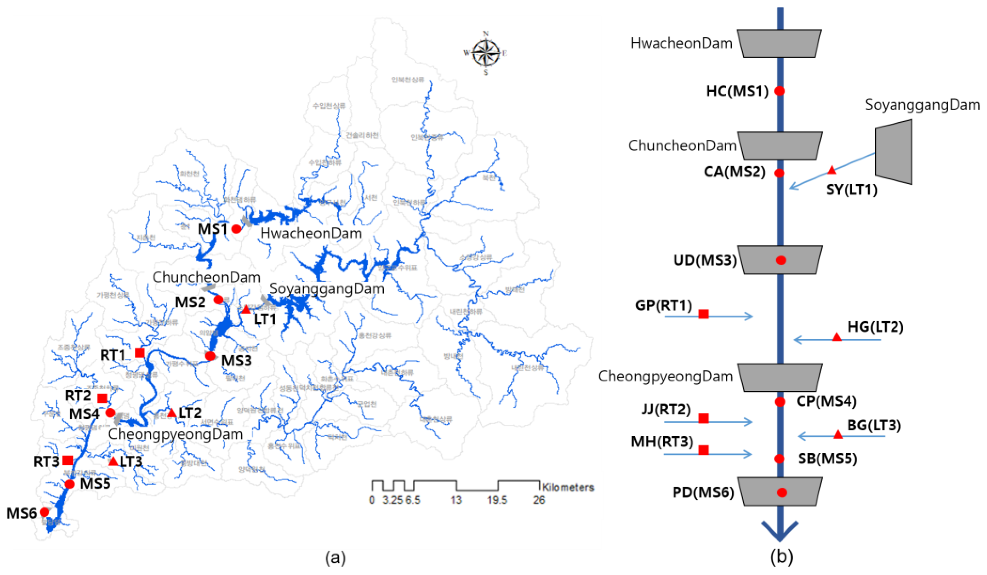
2.1. Study Site

The Bukhan River originates in Gangwon-do and, along with the Namhan River, is one of two major tributaries of the Han River. In this study, we used weekly water quality data of the Bukhan River from 2016 to 2018 obtained from the WIS. There are total of 12 monitoring stations (Figure 1;

Table 1. Abbreviations of water quality monitoring stations of the Bukhan River.

	Station	Abbreviation		Station	Abbreviation
Main stream (MS)	Hwacheon	HC (MS1)	Right tributary (RT)	Gapyeongcheon3 (stream)	GP (RT1)
	Chuncheon A	CA (MS2)		Jojongcheon3 (stream)	JJ (RT2)
	UiamDam	UD (MS3)		Mukhyeoncheon (stream)	MH (RT3)
	Cheongpyeong	CP (MS4)	Left tributary (LT)	Soyanggang2 (river)	SY (LT1)
	Sambongli	SB (MS5)		Hongcheongang6 (river)	HG (LT2)
	PaldangDam	PD (MS6)		Byeoggyecheon (stream)	BG (LT3)

), including 6 main stations (Hwacheon, Chuncheon A, UiamDam, Cheongpyeong, Sambongli, and PaldangDam) and 6 tributary stations (Gapyeongcheon3(stream), Jojongcheon3(stream), Mukhyeoncheon(stream), Soyanggang2(river), Hongcheongang6(river), and Byeoggyecheon(stream)).

2.2. Data

In this study, nine water quality variables contained in the WIS were used, including hydrogen ion concentration, dissolved oxygen, biochemical oxygen requirements, chemical oxygen requirements, suspended solids, total nitrogen, total phosphorus, water temperature, and electrical conductivity (

Table 2. Characteristics of variables measured for the Bukhan River.

Variable	Description		Mean	SD
pH	Hydrogen Ion Concentration		8.05	0.45
DO	Dissolved Oxygen	mg/L	11.04	2.06
BOD	Biochemical Oxygen Demand	mg/L	0.98	0.92
COD	Chemical Oxygen Demand	mg/L	3.30	1.32
SS	Suspended Solid	mg/L	4.64	14.42
TN	Total Nitrogen	mg/L	2.46	1.99
TP	Total Phosphorus	mg/L	0.03	0.06
Temp	Temperature	°C	14.96	7.54
EC	Electrical Conductivity	μmhos/cm	152.76	86.24

).

Table 3. Characteristics of variables recorded by monitoring stations of the Bukhan River.

Mainstream
	Hwacheon			Chuncheon A			UiamDam
Variable	Mean	SD	N	Mean	SD	N	Mean	SD	N
pH	8.01	0.32	149	7.83	0.25	149	8.17	0.78	150
DO	11.10	1.78	149	10.43	2.10	149	11.60	2.68	150
BOD	0.53	0.25	149	0.59	0.17	149	1.31	0.55	150
COD	2.55	0.48	149	2.74	0.41	149	3.16	0.70	150
SS	1.92	1.59	149	2.56	1.99	149	4.05	9.37	150
TN	1.29	0.36	149	1.31	0.33	149	1.89	0.49	150
TP	0.01	0.01	149	0.01	0.02	149	0.02	0.02	150
Temp	13.91	6.20	149	13.71	5.89	149	12.89	6.64	150
EC	113.31	19.73	149	106.13	18.66	149	101.83	14.69	150
	Cheongpyeong			Sambongli			PaldangDam
Variable	Mean	SD	N	Mean	SD	N	Mean	SD	N
pH	8.11	0.32	149	7.79	0.44	155	7.82	0.42	155
DO	10.86	1.84	149	10.40	1.74	155	10.10	2.40	155
BOD	1.00	0.49	149	0.90	0.29	155	1.16	0.38	155
COD	3.50	0.66	149	3.46	0.49	155	3.79	0.52	155
SS	3.91	4.66	149	3.37	4.39	155	5.16	3.52	155
TN	1.87	0.38	149	1.88	0.33	155	2.20	0.41	155
TP	0.02	0.02	149	0.02	0.01	155	0.03	0.02	155
Temp	16.58	7.42	149	15.64	7.69	155	13.78	7.72	155
EC	112.41	16.06	149	127.52	27.20	155	198.62	37.69	155
Right tributary
	Gapyeongcheon3 (stream)			Jojongcheon3 (stream)			Mukhyeoncheon (stream)
Variable	Mean	SD	N	Mean	SD	N	Mean	SD	N
pH	8.15	0.34	149	8.31	0.44	149	7.82	0.30	153
DO	11.37	1.90	149	11.56	2.03	149	10.34	1.34	153
BOD	0.66	0.35	149	0.94	0.40	149	2.38	1.75	153
COD	2.62	1.63	149	3.15	0.88	149	6.17	1.94	153
SS	4.32	21.12	149	5.74	8.00	149	12.08	38.83	153
TN	1.90	0.47	149	2.60	0.81	149	3.34	3.50	153
TP	0.01	0.03	149	0.03	0.02	149	0.10	0.13	153
Temp	17.36	8.37	149	17.61	8.62	149	18.29	6.11	153
EC	108.94	28.74	149	182.71	36.91	149	406.71	91.45	153
Left tributary
	Soyanggang2 (river)			Hongcheongang6 (river)			Byeoggyecheon (stream)
Variable	Mean	SD	N	Mean	SD	N	Mean	SD	N
pH	8.00	0.40	154	8.21	0.24	149	8.28	0.33	153
DO	12.14	1.42	154	10.34	2.00	149	11.37	1.94	153
BOD	0.36	0.12	154	0.62	0.31	149	0.61	0.41	153
COD	2.78	0.41	154	3.00	0.74	149	2.78	1.12	153
SS	1.70	1.86	154	2.94	5.91	149	3.22	5.34	153
TN	1.59	0.15	154	2.65	0.74	149	1.79	0.55	153
TP	0.01	0.01	154	0.02	0.02	149	0.02	0.03	153
Temp	9.50	3.14	154	16.92	8.12	149	15.10	8.27	153
EC	79.88	8.13	154	180.59	39.28	149	118.48	31.62	153

shows the basic statistics and lengths of the data from the 12 stations. The Euclidean algorithm requires data of the same length for comparison, whereas the DTW algorithm can be used even if data lengths are different. Therefore, when using Euclidean algorithms, only data collected at the same time at all stations were used for analysis. If data were missing at even one station, the data at that point were removed for all stations. As a result, a total of 1680 data points were analyzed using the Euclidean algorithm, and 1814 data points were analyzed using the DTW algorithm.

Missing Data

This study used the Kalman replacement method, which replaces missing values based on the Kalman filter, to replace missing values in the data. The Kalman filter removes data noise and predicts future data by using historical and newly measured data in a dynamic linear model that changes over time.

The Kalman filter repeats the prediction and update phases to predict variables. In the prediction step, the state of variable at time t and the preliminary estimate of the error covariance are calculated using the state variable at time t−1. Then, in the update step, the estimation is updated by reflecting the Kalman gain and the observation at time t in the prior estimate. The updated estimate is called the posterior estimate. Figure 2 visualizes the missing data values used in this study; the ratio of missing values for the whole dataset was 16.5%.

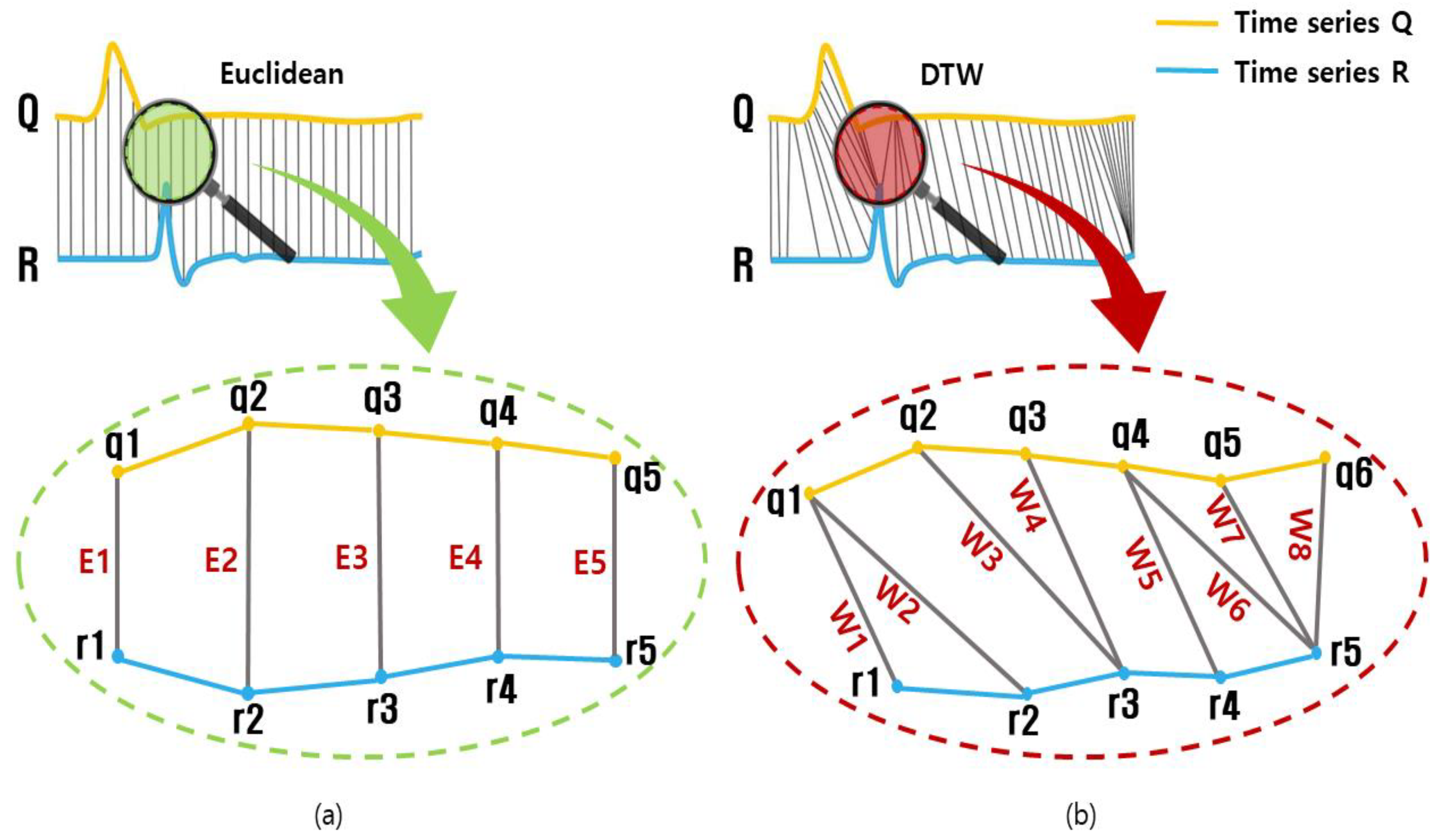
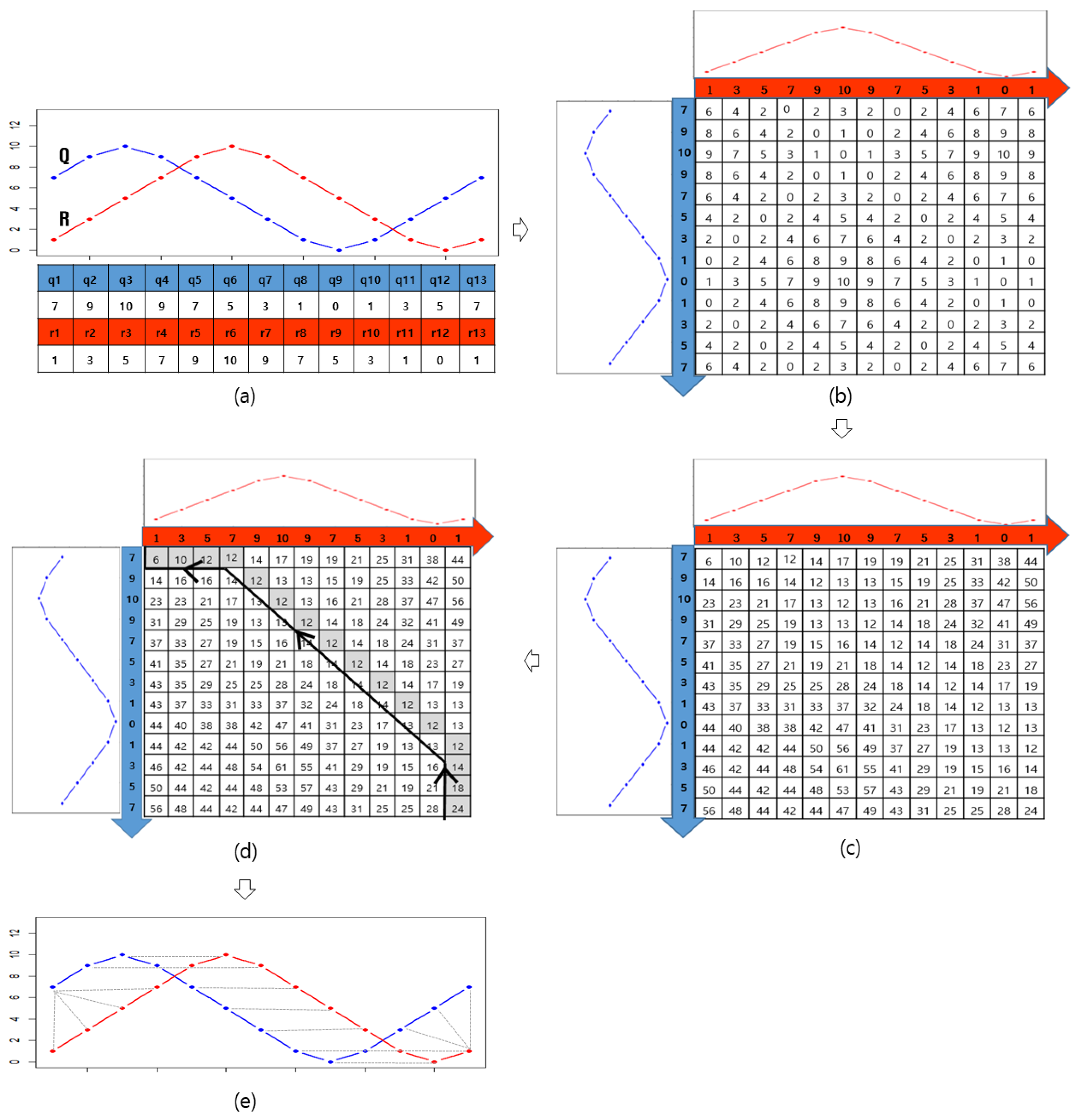
2.3. Dynamic Time Warping

This study conducted K-medoids cluster analysis using the Euclidean algorithm and the DTW algorithm for water quality network data using ‘dtw’ package in the statistical program R (ver 3.6.1).

The Euclidean algorithm compares two time series one-on-one at the same time; therefore, the lengths of the two time series must be the same. Therefore, if the length of the time series being compared is different, the length must be transformed, which inevitably leads to loss of information. In addition, if the values of two stations at the same time were measured with a delay (e.g., the distance between the stations), the similarity between the two time series is low, even if they are of the same time series.

In contrast, the DTW algorithm matches time series in a direction that minimizes the distance between two time series, allowing data at different points in time to be compared. Thus, when comparing time series of different lengths through the DTW algorithm, they can be compared without loss of data. Furthermore, the DTW algorithm has the advantage of being relatively robust in distortion and deformation. Figure 3 shows a conceptual plot of the Euclidian and DTW algorithms, assuming that there are two time series Q and R with different lengths m, n. ‘E’ and ‘W’ are lines showing mapping between two points that each methodology compares. Since Euclidean distance only compares data at the same time point, ‘E’ looks like a vertical line. On the other hand, since DTW can also compare data at different time, ‘W’ may not be a vertical line, unlike ‘E’.

Assuming two time series Q and R with different lengths of m, n (Figure 4a), the DTW algorithm proceeds as follows:

Step 1 (Figure 4b): Create local cost matrix C, also called the local distance matrix, by using the local cost function c, which represents the Euclidean distance between two points (q,r). For two time series Q and R, the local distance function c and Cost matrix C are defined as follows:

$$\mathrm{C}\left(\mathrm{i},\mathrm{j}\right)=\mathrm{c}\left({\mathrm{q}}_{\mathrm{i}},{\mathrm{r}}_{\mathrm{j}}\right)=\sqrt{{\left({\mathrm{q}}_{\mathrm{i}}-{\mathrm{r}}_{\mathrm{i}}\right)}^2}$$

(1)

where c is the distance between any two points of time series Q and R, and i and j are the indices representing the i-th and j-th points of each time series. The c is the distance function and has a smaller value if the comparison targets are similar, and a larger value if they are different. If the DTW algorithm is applied to multivariate time-series data with V variables, the cost distance is calculated by calculating the local distances for each variable at the same time and summing them as follows:

$$\mathrm{C}\left(\mathrm{i},\mathrm{j}\right)={\displaystyle \sum }_{\mathrm{v}=1}^{\mathrm{V}}\mathrm{c}\left({\mathrm{q}}_{\mathrm{iv}},{\mathrm{r}}_{\mathrm{jv}}\right)=\sqrt{{\displaystyle \sum }_{\mathrm{v}=1}^{\mathrm{V}}{\left({\mathrm{q}}_{\mathrm{iv}}-{\mathrm{r}}_{\mathrm{jv}}\right)}^2}$$

(2)

Step 2 (Figure 4c): Create a global cost matrix M. First, the first row and first column of matrix M are calculated as follows:

$$\mathrm{M}\left(\mathrm{i},\mathrm{j}\right)=\{\begin{array}{c}\mathrm{C}\left(1,\mathrm{j}\right)+\mathrm{M}\left(1,\mathrm{j}-1\right)\\ \mathrm{C}\left(\mathrm{i},1\right)+\mathrm{M}\left(\mathrm{i}-1,1\right)\end{array}$$

(3)

At this time, M(1,1) = C(1,1). Then, calculate the rest of the matrix as follows:

$$\mathrm{M}\left(\mathrm{i},\mathrm{j}\right)=\mathrm{C}\left(\mathrm{i},\mathrm{j}\right)+\min \left[\mathrm{M}\left(\mathrm{i}-1,\mathrm{j}-1\right),\mathrm{M}\left(\mathrm{i}-1,\mathrm{j}\right),\mathrm{M}\left(\mathrm{i},\mathrm{j}-1\right)\right]$$

(4)

Step 3 (Figure 4d): Find the optimum warping path to meet the constraints mentioned by Sakoe et al. [7] in global cost matrix M. The warping path, which satisfies constraints, exists in a variety of ways. The DTW algorithm considers that the path where the sum of the distances between two time series is the minimum is the optimal warping path of the two time series. Mapping two time series through a warping path is shown in Figure 4e.

2.4. Clustering Method

Clustering is a multivariate data analysis method that groups objects into several clusters based on similarities between objects through distance measurements and identifies the characteristics of each cluster. At this time, objects with high similarity share the same cluster and those with low similarity have different clusters. In other words, clusters are formed so that the variance of data within a cluster is minimal and the variance between clusters is maximal. Cluster analysis includes various methods such as K-means clustering, hierarchical clustering, K-medoids clustering, the Fuzzy algorithm, etc., and uses only given data without prior information about the data.

The K-medoids algorithm used in this study was proposed by Kaufman et al. [12] and is a method of forming a cluster using medoid, a representative object located at the center of the cluster. The K-medoids algorithm is also called the Partitioning Around Medoids (PAM) algorithm, and the process of forming a cluster is as follows. Initially, randomly select k medoids and assign the remaining objects to clusters with the nearest medoid. Then, for each cluster, the object with the smallest mean of distance to all objects is set to the new center medoid. The remaining objects are assigned clusters with the nearest medoid again. This process is repeated until the new medoid and existing medoid are identical, and the cluster at the end of the iterative process is the optimal K-medoids cluster. The K-medoids algorithm repeatedly replaces one of the non-medoid objects with a medoid, minimizing the distance value between the objects forming the same cluster. This method represents an improvement on the k-means algorithm, which is greatly affected by outliers; it is less sensitive to outliers because it does not use the average as the central object. PAM cluster analysis were performed using the ‘dtwclust’ package in R, and since the units of the water quality variables are all different, the distance calculation and cluster analysis were performed after normalization for each variable.

2.5. Clustering Validation Index

The Clustering Validation Index (CVI), which is used to determine the optimal number of clusters, was used [13,14]. CVI is an indicator of how well clusters are formed. In this study, six internal CVIs were used; they were calculated based solely on data and cluster results. The CVIs were the Silhouette (Sil) proposed by Rousseeuw [15], the Calinski-Harabasz (CH) proposed by Caliński et al. [16], the Dunn (D) proposed by Dunn [17], the Davies Bouldin (DB) proposed by Davies et al. [18], the COP index proposed by Gurrutxaga et al. [19], and the Modified Davies Bouldin (MDB) proposed by Kim et al. [20]. The smaller the values of Sil, CH, and D, the larger the values of DB, MDB, and COP, and the better the clusters were formed. CVI were performed using the ‘dtwclust’ package in R.

3. Results

3.1. Optimization CVI

The number of clusters was set in advance from two to five, and the optimal number of clusters was determined based on the CVI (

Table 4. Clustering Validation Index for the Euclidean and Dynamic Time Warping (DTW) Algorithms. Shading represents the largest value (DB, MDB, COP) or the smallest value (Sil, CH, D) of an index.

# of Cluster		Clustering Validation Index
		Sil	CH	DB	MDB	D	COP
Euclidean algorithm	2	0.160	12.436	1.257	1.257	0.701	0.668
	3	0.140	6.578	1.245	1.245	0.776	0.532
	4	0.131	4.430	1.054	1.091	0.776	0.464
	5	0.050	3.384	0.939	1.066	0.659	0.423
DTW algorithm	2	0.106	7.649	1.493	1.493	0.763	0.681
	3	0.128	3.981	1.338	1.353	0.824	0.594
	4	0.130	2.737	1.116	1.144	0.824	0.514
	5	0.044	3.064	1.028	1.135	0.624	0.476

). Typically, many CVIs are utilized and compared to each other, and a majority vote can be used to determine the final outcome [13,14]. Therefore, the optimal number of clusters was found to be five for both algorithms. Missing data values were replaced using Kalman filters, and standardized data were used for analysis.

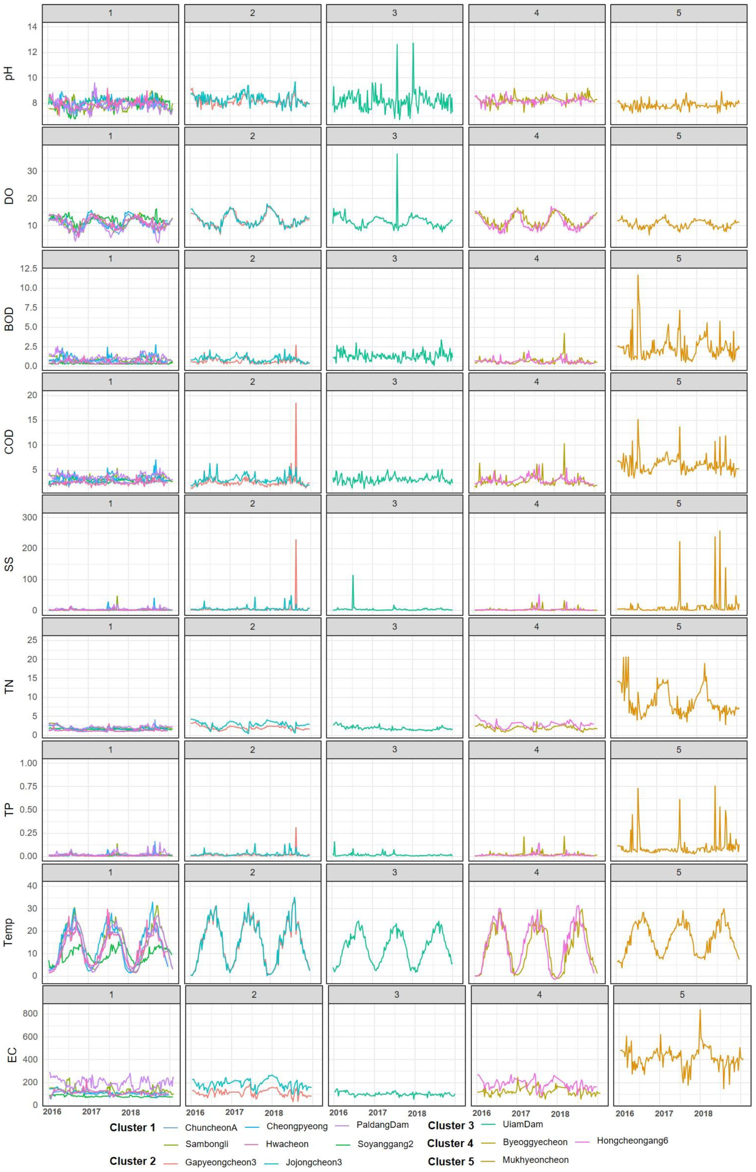
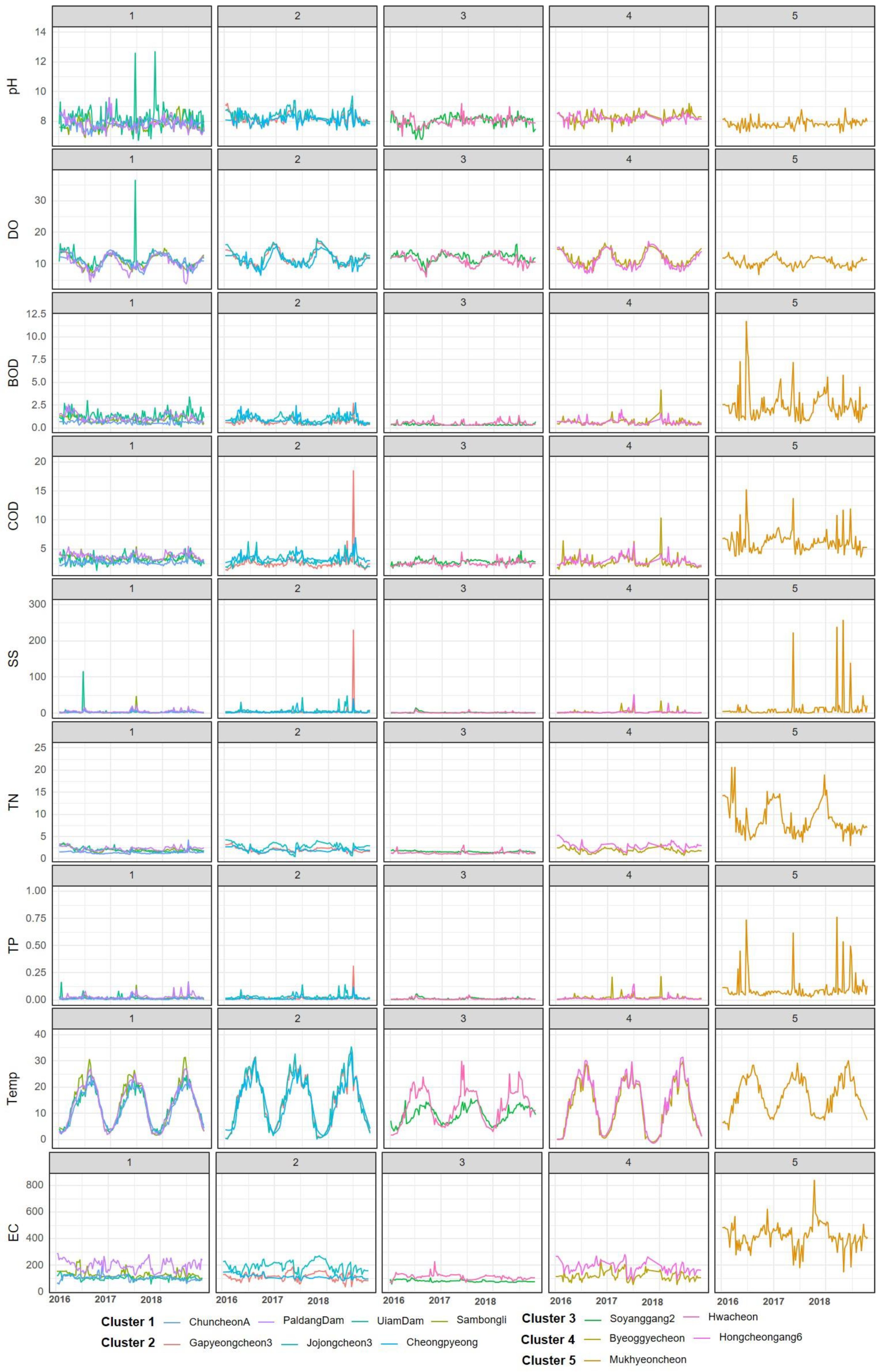
3.2. Comparison of the Euclidean and Dynamic Time Warping Algorithms

Water quality measuring stations were divided into five clusters as shown in Figure 5. Using the Euclidean algorithm, Mukhyeoncheon formed a cluster alone; Sambongli, UiamDam, Chuncheon A, and PaldangDam formed a cluster; Gapyeongcheon3, Jojongcheon3, and Cheongpyeong formed a cluster; and finally, Byeoggyecheon and Hongcheongang6 formed a cluster. However, when the DTW algorithm was used, Gapyeongcheon3 and Jojongcheon3(stream) were separated from Cheongpyeong, while UiamDam was separated from other measuring stations in the mainstream. Cheongpyeong and Hwacheon formed a cluster with Soyanggang2, Chuncheon A, and PaldangDam. As for the Euclidean algorithm, Mukhyeoncheon formed a cluster alone. Unlike the Euclidean algorithm, UiamDam also formed a cluster alone.

For clusters formed with both algorithms, there was a statistically significant mean difference according to clusters formed from all variables. To examine in detail the mean differences according to the cluster, Tukey’s test was used at a significance level of 0.05 (

Table 5. Post hoc test results for cluster analysis using the Euclidean and Dynamic Time Warping (DTW) algorithms.

		Euclidean Algorithm					DTW Algorithm
pH	Cluster	4	2	3	1	5	4	2	3	1	5
	Mean	8.251	8.192	8.017	7.915	7.826	8.255	8.242	8.174	7.932	7.829
	Group	a	a	b	c	c	a	a	a	b	c
DO	Cluster	2	3	4	1	5	2	4	3	1	5
	Mean	11.798	11.718	11.603	10.863	10.599	12.047	11.613	11.598	11.076	10.596
	Group	a	a	a	b	b	a	a	ab	bc	c
BOD	Cluster	5	1	2	4	3	5	3	2	1	4
	Mean	2.466	0.995	0.838	0.652	0.437	2.420	1.313	0.723	0.752	0.647
	Group	a	b	c	d	e	a	b	c	cd	d
COD	Cluster	5	1	2	4	3	5	3	1	4	2
	Mean	6.229	3.274	3.016	2.883	2.645	6.200	3.157	3.116	2.874	2.810
	Group	a	b	c	c	d	a	b	b	c	c
SS	Cluster	5	2	1	4	3	5	2	3	1	4
	Mean	12.753	4.619	3.744	2.973	1.180	12.393	5.017	4.055	3.016	3.004
	Group	a	b	bc	bc	c	a	b	b	b	b
TN	Cluster	5	4	2	1	3	5	2	4	3	1
	Mean	8.896	2.348	2.204	1.838	1.432	8.955	2.363	2.348	1.890	1.708
	Group	a	b	b	c	d	a	b	b	c	c
TP	Cluster	5	1	2	4	3	5	2	4	3	1
	Mean	0.104	0.019	0.019	0.018	0.011	0.102	0.021	0.018	0.017	0.016
	Group	a	b	b	bc	c	a	b	b	b	b
Temp	Cluster	5	2	4	1	3	5	2	4	3	1
	Mean	16.725	14.945	13.241	13.097	11.006	16.691	15.263	13.205	12.887	12.735
	Group	a	a	b	b	c	a	a	b	b	b
EC	Cluster	5	4	2	1	3	5	4	2	1	3
	Mean	418.594	156.011	137.684	132.976	96.678	418.398	155.536	150.155	123.336	101.827
	Group	a	b	c	c	d	a	b	b	c	d

). When statistically significant differences were found, the groups were expressed differently; a, b, c, d were expressed in order from the highest group to the lowest group.

When using the Euclidean algorithm, Cluster 1 (Sambongli, UiamDam, Chuncheon A, and PaldangDam) had lower average values of pH and DO. In contrast, Cluster 4 (Byeoggyecheon and Hongcheongang6) had high average values of pH and DO. Cluster 2 (Gapyeongcheon3, Jojongcheon3, and Cheongpyeong) had high pH, DO, and Temp. Cluster 3 (Soyanggang2 and Hwacheon) showed high average values of DO and low average values of BOD, COD, SS, TN, TP, Temp, and EC. Cluster 5 (Mukhyeoncheon) had low pH and DO and high values for other water quality variables; among them, BOD, COD, SS, TN, TP, and EC showed a very significant difference from other clusters.

When using the DTW algorithm, Cluster 1 (Soyanggang2 and the mainstream except UiamDam) showed low TN and Temp. Cluster 2 (Gapyeongcheon3 and Jo Jongcheon3) showed high pH, DO, and Temp, and low COD. Cluster 3 (UiamDam) showed high pH and low TN, Temp, and EC. Cluster 4 (Byeoggyecheon and Hongcheongang6) has high pH and DO, and low BOD, COD, and Temp averages. Cluster 5 (Mukhyeoncheon) showed the same characteristics as that formed using the Euclidian algorithm.

Table 6. Cluster characteristics for the Euclidean and Dynamic Time Warping (DTW) algorithms.

	Cluster	Station	Variable	Location
			Characteristics	Characteristics
Euclidean algorithm	1	CA(MS2), UD(MS3), SB(MS5), PD(MS6)	low: pH, DO	Mainstream
	2	GP(RT1), JJ(RT2), CP(MS4),	high: pH, DO, Temp	Right tributary Mainstream Midstream
	3	SY(LT1), HC(MS1)	high: DO	Left tributary Mainstream Upstream
			low: BOD, COD, SS, TN, TP, Temp, EC
	4	BG(LT3), HG(LT2)	high: pH, DO	Left downstream tributary
	5	MH(RT3)	high: BOD, COD, SS, TN, TP, Temp, EC	Right downstream tributary
			low: pH, DO
DTW algorithm	1	HC(MS1), CA(MS2), CP(MS4), SB(MS5), PD(MS6), SY(LT1)	low: TN, Temp	Left tributary Mainstream
	2	GP(RT1), JJ(RT2)	high: pH, DO, Temp	Right midstream tributary
			low: COD
	3	UD(MS3)	high: pH	Mainstream
			low: TN, Temp, EC
	4	HG(LT2), BG(LT3)	high: pH, DO	Left downstream tributary
			low: BOD, COD, Temp
	5	MH(RT3)	high: BOD, COD, SS, TN, TP, Temp, EC	Right downstream tributary
			low: pH, DO

shows cluster-specific variable characteristics for each algorithm.

Both the Euclidean and DTW algorithms included Byeoggyecheon and Hongcheongang6 in the same cluster, but the water quality characteristics of the clusters differed. This difference reflects the need for data removal when using the Euclidean algorithm, and shows that data distortion is inevitable when the time series being compared have different lengths.

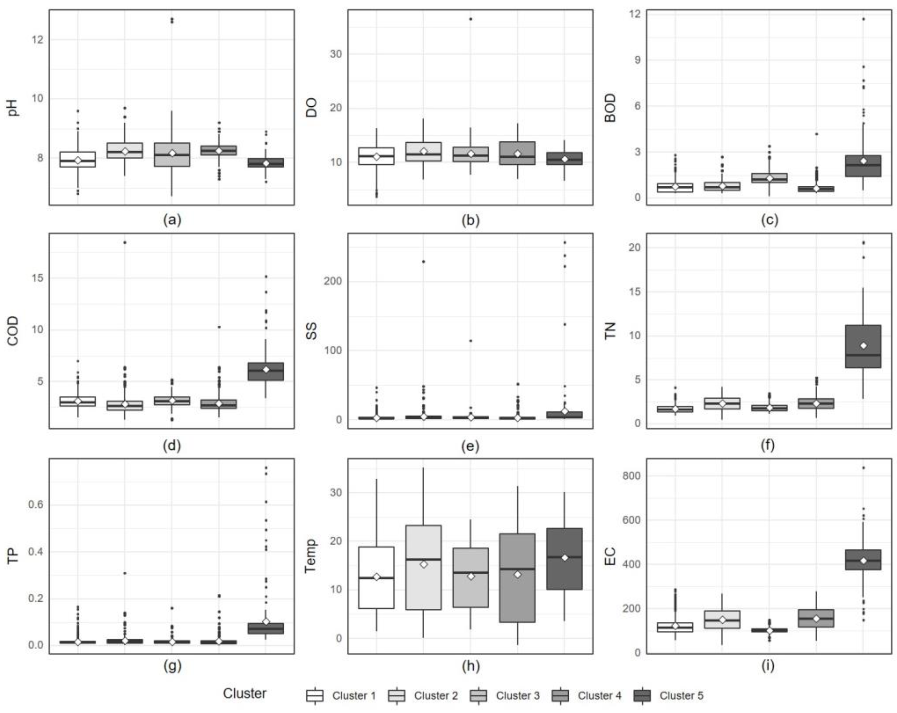
3.3. Comparison of Water Quality Characteristics for Each Cluster

Figure 6 and Figure 7 show cluster-specific boxplots for each variable when the 12 streams are divided into 5 clusters using K-medoids cluster analysis with the Euclidian and DTW algorithms, respectively. When using the Euclidian algorithm (Figure 6), Mukhyeoncheon (Cluster 5) had a greater value and deviation than other streams belonging to other clusters in terms of BOD, COD, TN, TP, and EC. The result is similar using the DTW algorithm (Figure 7).

Figure 8 and Figure 9 show cluster-specific time series plots for each variable when the 12 streams were divided into 5 clusters through K-medoids cluster analysis using the Euclidian and DTW algorithms, respectively. In both cases, Cluster 5 (Mukhyeoncheon) showed unusual water parameter patterns compared with the other streams. Regardless of cluster, water temperature was similar for most rivers, although Soyanggang2 had unusually low water temperatures compared with the other streams.

4. Discussion

4.1. Comparison of Clustering and Water Quality Patterns

The Euclidean algorithm, which aligns the i-th point of one sequence with the i-th point of the other sequence, can cause low similarity. Because of this, DTW, which allows nonlinear alignment, is often used instead of Euclidean algorithm in various fields. In hydrology, Ouyang et al. [11] used DTW algorithm instead of Euclidian algorithm for similarity search and pattern discovery in the hydrologic time series data. Chotirat et al. [20] classified time series data obtained from the video data with DTW-applied model and compared the model performance with the Euclidean based model.

So, this study applied Euclidean and DTW distance algorithms to water quality data to determine similarities among water quality at different monitoring stations and to identify the characteristics of water quality variables by cluster.

The Euclidean method clustered stations from the mainstream, left tributary, and right tributary together. In contrast, DTW formed three clusters that generally reflected the mainstream, left tributary, and right tributary (except for Soyanggang2, UiamDam, and Mukhyeoncheon). As such, the DTW approach better reflected the regional characteristics of the watersheds and hydraulic environments. Both algorithms showed statistically significant mean differences across clusters in all variables, and both clustered Byeoggyecheon and Hongcheongang6 together. However, the water quality characteristics of the clusters differed, highlighting the impact of unavoidable data removal when using the Euclidean algorithm, resulting in a distortion of water quality characteristics.

Cluster 1 of the DTW classification, representing mainstream stations, shows relatively better water quality than Cluster 2 (left tributary) and Cluster 4 (the right tributary). However, while the Soyanggang2 monitoring station belongs to the left-hand tributary, it was classified into the mainstream cluster. The reason for this is that the measuring station is located directly downstream of the Soyanggang Dam, a large-scale dam with a storage capacity of 29 million m³. The dam has relatively good water quality because it is located in a water resource protection zone and is used as a source of drinking water. As such, the water quality of Soyanggan2 monitoring station is relatively better compared with the monitoring stations in Cluster 2 (i.e., the other stations on the left-hand tributary), and so it is was classified into the mainstream cluster, for which stations show better water quality.

Despite being a right-hand tributary, Mukhyeoncheon was classified as a separate cluster. The concentrations of BOD and COD (representative of pollution by organic matter), and of TN and TP (representative of pollution by nutrients) averaged 2.38 mg/L, 6.17 mg/L, 3.34 mg/L, and 0.1 mg/L, respectively. This demonstrates markedly higher levels of contamination than other stations, particularly those in Cluster 4 (the other right-hand tributaries).

UiamDam belongs to the mainstream, but its BOD, COD, TN, TP, and SS values are all greater than those of other stations in DTW Cluster 1 (i.e., other mainstream stations). In particular, the average BOD was 1.31 mg/L, which is significantly higher than the average of the stations corresponding to DTW Cluster 1.

The Bukhan River Basin has a low population density and few industrial facilities. The Mukhyeoncheon and UiamDam flow along the densely populated metropolitan cities in the Basin and are affected by various downtown streams. We believe that various point/non-point pollutants in these urban areas affect the water quality at these stations, which explains why they are not clustered with other stations from the same geographical area.

Long-term observational data obtained from on-site monitoring networks are critical for the proper management of water quality and ecosystems. However, the operation of on-site monitoring stations is not always possible due to limited budget. The DTW analysis in this study provides useful information for understanding the similarity or difference in water parameter values between different locations. Thus, the number and location of required monitoring stations can be adjusted to improve the efficiency of field monitoring network management.

4.2. Limits and Future Work

The main limitation of this study was a low number of samples, which reflects the relatively small-scale nature of the Bukhan River water system. As DTW takes a long time, with the calculation time increasing as the data volume increases, using a limited number of samples was necessary. However, in the future, analysis will be expanded to include more rivers. In addition, the water quality data used in this study included missing values owing to the failure of the measuring sensors and/or human error (e.g., lack of responsibility). If missing value significantly change time series trend, the reliability of the analysis results may be lowered.

In future studies, it may be possible to add variables such as chlorophyll-a and fecal coliforms, which were not used in the analysis owing to high rates of missing data, or to select proxy variables that reflect the characteristics of water quality variables. However, if the sources of stream pollution continue to increase, there is a limit to the efficacy of monitoring and improving water quality relied on general concentration regulation methods. To this end, the Ministry of Environment of South Korea is introducing and implementing a “Total Water Pollution Load Management System” that regulates the amount of pollution and reflects the emission of pollutants. The pollutant load data (including flow rate) were not utilized in this study because measurement frequency and measurement points remain limited. However, if sufficient data are secured in the future, it would be possible to add pollutant load data to reflect the amount of pollutant discharge. We will also plan to compare the result of dynamic PCA with the one of DTW.

5. Conclusions

Proper network installation and removal is an important part of water quality monitoring and network operation efficiency. To reduce the time and cost required to secure and monitor water quality data at locations where measurement is difficult, cluster analysis based on calculated similarity and dissimilarity between measuring stations can be used. Cluster analysis forms clusters based on the similarity measured according to distance, and so cluster results may vary depending on the type of distance. This study clustered water quality measuring stations of the Bukhan River water system using the K-medoids cluster analysis based on both the Euclidean and DTW algorithms.

The Euclidean algorithm compares the same time points of two time series and is limited by the fact that the lengths of the two time series must be the same. In contrast, the DTW algorithm compares time series while changing the time point and can be used even if the lengths of the two time series are different. In water quality measurement network data, there is a time lag as water flows from upstream to downstream, and the length of the data may be different for each measuring station owing to failures of the measuring device, etc. Therefore, when clustering water quality data from a measurement network, it should be preferable to use the DTW algorithm.

Our results show that the Euclidean algorithm formed clusters by mixing mainstream and tributary stations; the mainstream stations were largely divided into three different clusters. In contrast, the DTW algorithm formed clear clusters by reflecting the characteristics of water quality and watershed. Furthermore, because the Euclidean algorithm requires the lengths of the time series to be the same, data loss was inevitable. As a result, even where clusters were the same as those obtained by DTW, the characteristics of the water quality variables in the cluster differed.

References

1. Driver, H.E.; Kroeber, A.L. Quantitative Expression of Cultural Relationships. In American Archeology and Ethnology; University of California Press: Berkeley, CA, USA, 1932; Volume 31, pp. 211–256. [Google Scholar]
2. Aubert, A.H.; Tavenard, R.; Emonet, R.; de Lavenne, A.; Malinowski, S.; Guyet, T.; Quiniou, R.; Odobez, J.-M.; Merot, P.; Gascuel-Odoux, C. Clustering flood events from water quality time series using Latent Dirichlet Allocation model. Water Resour. Res. 2013, 49, 8187–8199. [Google Scholar] [CrossRef]
3. Lyra, G.B.; Oliveira-Júnior, J.F.; Zeri, M. Cluster analysis applied to the spatial and temporal variability of monthly rainfall in Alagoas state, Northeast of Brazil. Int. J. Climatol. 2014, 34, 3546–3558. [Google Scholar] [CrossRef]
4. Emad, A.M.S.A.-H.; Ahmed, M.T.; Eethar, M.A.-O. Assessment of water quality of Euphrates River using cluster analysis. J. Environ. Prot. 2012, 3, 1629–1633. [Google Scholar] [CrossRef] [Green Version]
5. Azhar, S.C.; Aris, A.Z.; Yusoff, M.K.; Ramli, M.F.; Juahir, H. Classification of river water quality using multivariate analysis. Procedia Environ. Sci. 2015, 30, 79–84. [Google Scholar] [CrossRef] [Green Version]
6. Bellman, R.; Kalaba, R. On adaptive control processes. IRE Trans. Autom. Control 1959, 4, 1–9. [Google Scholar] [CrossRef]
7. Sakoe, H.; Chiba, S. Dynamic programming algorithm optimization for spoken word recognition. IEEE Trans. Acoust. Speech Signal Process. 1978, 26, 43–49. [Google Scholar] [CrossRef] [Green Version]
8. Dürrenmatt, D.J.; Del Giudice, D.; Rieckermann, J. Dynamic time warping improves sewer flow monitoring. Water Res. 2013, 47, 3803–3816. [Google Scholar] [CrossRef] [PubMed]
9. Woo, H.; Boccelli, D.L.; Uber, J.G.; Janke, R.; Su, Y. Dynamic time warping for quantitative analysis of tracer study time-series water quality data. J. Water Res. Plan. Manag. 2019, 145, 04019052. [Google Scholar] [CrossRef]
10. Dupas, R.; Tavenard, R.; Fovet, O.; Gilliet, N.; Grimaldi, C.; Gascuel-Odoux, C. Identifying seasonal patterns of phosphorus storm dynamics with dynamic time warping. Water Resour. Res. 2015, 51, 8868–8882. [Google Scholar] [CrossRef] [Green Version]
11. Ouyang, R.; Ren, L.; Cheng, W.; Zhou, C. Similarity search and pattern discovery in hydrological time series data mining. Hydrol. Process. Int. J. 2010, 24, 1198–1210. [Google Scholar] [CrossRef]
12. Kaufman, L.; Rousseeuw, P.J. References. In Finding Groups in Data: An Introduction to Cluster Analysis; John Wiley & Sons, Inc.: Hoboken, NY, USA, 1990; ISBN 978-0-47031680-1. [Google Scholar]
13. Sardá-Espinosa, A. Comparing time-series clustering algorithms in r using the dtwclust package. R package vignette. Pattern Recognit. 2017, 12, 41. [Google Scholar] [CrossRef]
14. Arbelaitz, O.; Gurrutxaga, I.; Muguerza, J.; PéRez, J.M.; Perona, I. An extensive comparative study of cluster validity indices. Pattern Recognit. 2013, 46, 243–256. [Google Scholar] [CrossRef]
15. Rousseeuw, P.J. Silhouettes: A graphical aid to the interpretation and validation of cluster analysis. J. Comput. Appl. Math. 1987, 20, 53–65. [Google Scholar] [CrossRef] [Green Version]
16. Caliński, T.; Harabasz, J. A dendrite method for cluster analysis. Commun. Stat. Theory Methods 1974, 3, 1–27. [Google Scholar] [CrossRef]
17. Dunn, J.C. Well-separated clusters and optimal fuzzy partitions. J. Cybern. 1974, 4, 95–104. [Google Scholar] [CrossRef]
18. Davies, D.L.; Bouldin, D.W. A cluster separation measure. IEEE Trans. Pattern Anal. Mach. Intell. 1979, 1, 224–227. [Google Scholar] [CrossRef] [PubMed]
19. Gurrutxaga, I.; Albisua, I.; Arbelaitz, O.; Martín, J.I.; Muguerza, J.; Pérez, J.M.; Perona, I. SEP/COP: An efficient method to find the best partition in hierarchical clustering based on a new cluster validity index. Pattern Recognit. 2010, 43, 3364–3373. [Google Scholar] [CrossRef]
20. Kim, M.; Ramakrishna, R.S. New indices for cluster validity assessment. Pattern Recognit. Lett. 2005, 26, 2353–2363. [Google Scholar] [CrossRef]
Figure 1. Bukhan River drainage system (a). Map-based drainage system schematic and (b) schematic diagram of the drainage system.
Water 12 02411 g001
Figure 2. Map of missing data.
Water 12 02411 g002
Figure 3. Aligning rules for the (a) Euclidean (E) algorithm and (b) Dynamic Time Warping (DTW) algorithm. ‘E’ and ‘W’: lines showing mapping between two points that each methodology compares.
Water 12 02411 g003
Figure 4. Illustration of global cost matrix and warping path of the classic Dynamic Time Warping (DTW) algorithm; (a). Two time series (b). Local cost matrix (c). Global cost matrix (d). Optimal warping path (e). DTW alignment.
Water 12 02411 g004
Figure 5. Cluster formation using the (a) Euclidean algorithm and (b) Dynamic Time Warping (DTW) algorithm.
Water 12 02411 g005
Figure 6. Cluster-specific boxplots for each variable when using the Euclidean algorithm about (a) pH, (b) DO, (c) BOD, (d) COD, (e) SS, (f) TN, (g) TP, (h) Temp, and (i) EC.
Water 12 02411 g006
Figure 7. Cluster-specific boxplots for each variable when using the Dynamic Time Warping (DTW) algorithm about (a) pH, (b) DO, (c) BOD, (d) COD, (e) SS, (f) TN, (g) TP, (h) Temp, and (i) EC.
Water 12 02411 g007
Figure 8. Cluster-specific time series plots for each variable observed between 2016 and 2018 when using the Euclidean algorithm about Cluster 1 (1), Cluster 2 (2), Cluster 3 (3), Cluster 4 (4), and Cluster 5 (5).
Water 12 02411 g008
Figure 9. Cluster-specific time series plots for each variable observed between 2016 and 2018 when using the Dynamic Time Warping (DTW) algorithm about Cluster 1 (1), Cluster 2 (2), Cluster 3 (3), Cluster 4 (4), and Cluster 5 (5).
Water 12 02411 g009