Understanding the Biogeochemical Impacts of Fish Farms Using a Benthic-Pelagic Model

Abstract

Sustainable development of the salmon farming industry requires knowledge of the biogeochemical impacts of fish farm emissions. To investigate the spatial and temporal scales of farm impacts on the water column and benthic biogeochemistry, we coupled the C-N-P-Si-O-S-Mn-Fe transformation model BROM with a 2-dimensional benthic-pelagic transport model (2DBP), considering vertical and horizontal transport in the water and upper 5 cm of sediments along a 10 km transect centered on a fish farm. The 2DBP model was forced by hydrophysical model data for the Hardangerfjord in western Norway. Model simulations showed reasonable agreement with field data from the Hardangerfjord in August 2016 (correlations between the model and observations were significant for most variables, and model biases were mostly <35%). The model predicted significant impacts on seafloor biogeochemistry up to 1 km from the fish farm (e.g., increased organic matter in sediments, oxygen depletion in bottom water and sediments, denitrification, metal and sulfur reduction), as well as detectable decreases in oxygen and increases in ammonium, phosphate and organic matter in the surface water near to the fish farm.

1. Introduction

Fish farming is an important global industry that is constantly developing to meet the demands of the global population [1,2]. Salmon aquaculture is a major industry in Norway, where approximately 1.3 million tons of fish are produced annually [3], accounting for 51% of the global cultured salmon market [4]. Although the industry has clear economic and food security benefits, it faces challenges connected with environmental management of aquaculture sites, including carrying capacity prediction, land-water interaction and multi-site effects [5]. Before the further expansion of industrial activities, it is important to investigate the potential impacts of increased concentrations of nutrients, pharmaceuticals and waste products being delivered to the coastal marine environment [6,7,8,9,10].

In Norwegian salmon farms, the grow-out phase is mostly carried out in open net pens in the sea and lasts 14–22 months depending on the site. After, the fish are slaughtered, the farm goes through a fallowing period of minimum two months, and, given satisfying results from the mandatory benthic monitoring program, the farm is re-stocked with fish. Before a fish farming company is granted a license to operate on a specific site, the prospective site must meet a range of requirements related to, e.g., current conditions, water quality and sediment chemistry and fauna conditions defined in NS9410:2016 Environmental monitoring of benthic impact from marine fish farms (https://www.standard.no/no/Nettbutikk/produktkatalogen/Produktpresentasjon/?ProductID=800604). During production, the farm releases a large amount of waste feed and fish feces that decomposes in the water column and settles on the seafloor, affecting oxygen and nutrient regimes [11]. Depending on the amount and duration of the releases, the assimilation capacity of the sediments, and the flushing ability of the recipient water body, biogeochemical conditions are affected and in the ‘worst-case’ can become anoxic, with dramatic consequences for seafloor ecosystems. Fish farming impacts on bottom biogeochemistry and ecosystems can be traced for up to 8 years after the cessation of farming [12].

Field and experimental studies at the seafloor have provided important insights into short-term effects of farm emissions (e.g., Reference [13]), but models can provide a more generalized and broader-scale (in space and time) view, and help to investigate biogeochemical mechanisms behind observed effects. Models are a cost-effective method to evaluate the impacts of site selection and production levels on the environment and can be used in Environmental Impact Assessments (EIAs).

To date, models of aquaculture impacts have focused primarily on the processes of waste generation, deposition, and accumulation ([5,12,14,15,16,17,18]; see also a recent review by Falconer et al., [17]). Much less effort has gone into modeling the decomposition and remineralization of fish farm waste, and the impacts of fish farm emissions on biogeochemical cycles (e.g., eutrophication) either in the sediments (e.g., Reference [18]) or in the water column [19,20,21]. Models that have included biogeochemical processes have tended to employ quite simplified representations, not considering the various alternative electron acceptors (nitrate, metal oxides, sulfate), and potential transformations of elements (e.g., the methylation of mercury) that can have major impacts on biogeochemical cycles and water quality, especially in cases of severe organic input that can lead to low oxygen conditions.

We have sought to understand the biogeochemical impacts of fish farming in a more realistic way, first by exploiting the detailed treatment of redox biogeochemistry within the bottom redox model (BROM) [22], and second by developing a fully-integrated representation of the water column and upper sediments (the 2-dimensional benthic-pelagic transport model, or 2DBP). The latter enables a full resolution of vertical water structure and benthic-pelagic interactions [23], while also resolving the basic mechanisms of horizontal dispersal within a simplified 2D spatial setting. Such a model will not predict detailed spatial distributions (maps) of impacts for particular farms; however, we argue that the simplified or “generalized” spatial setting is potentially useful for exploring mechanisms of biogeochemical impacts and for helping to guide general policy on fish farm emissions. A specific research goal of this paper is the estimation of the spatial and temporal scales of fish farm impacts on the water column and sediment biogeochemistry. In this work, the model was calibrated using field data collected around fish farms in Hardangerfjorden, a fjord with some of the largest concentrations of salmon farms in Norway. We demonstrate the model’s ability to predict biogeochemical impacts of fish farm emissions in the water column and upper sediments for the 10 years period and discuss key modeling uncertainties and observational data needs for improving mechanistic model predictions.

2. Materials and Methods

2.1. Modeling

We combined the biogeochemical module of BROM [22] with a new 2DBP model for vertical and horizontal transport of matter in the water column and upper sediments. The resulting benthic-pelagic model 2DBP-BROM is integrated into an existing modular platform (Framework for Aquatic Biogeochemical Modeling, FABM; [24]), and is therefore coded as a set of reusable components, including the offline transport driver 2DBP and BROM modules for the ecosystem and biogeochemical variables.

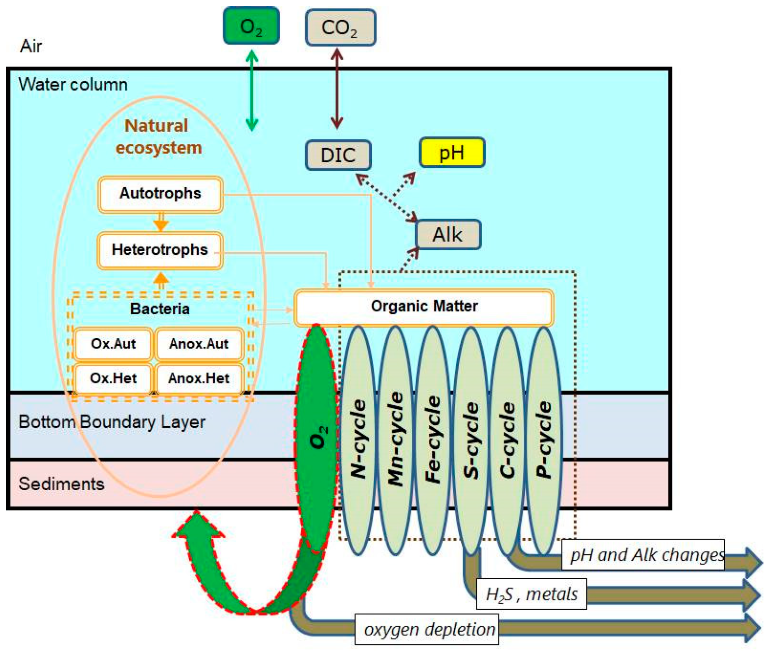
2.2. Biogeochemical Model BROM

The benthic-pelagic biogeochemical model BROM combines a relatively simple ecosystem model with a detailed biogeochemical model for the water column, benthic boundary layer, and sediments, with a focus on oxygen and redox state. BROM considers interconnected transformations of chemical species (N, P, Si, C, O, S, Mn, Fe) and resolves organic matter (OM) in nitrogen currency following Redfield ratios between the main nutrients (Figure 1). OM dynamics include parameterizations of production (via photosynthesis and chemosynthesis) and decay via oxic mineralization, denitrification, metal reduction, sulfate reduction and methanogenesis. To provide a detailed representation of changing redox conditions, OM in BROM is mineralized by several different electron acceptors, and dissolved oxygen is consumed during both mineralization of OM and oxidation of various reduced compounds. OM is described in the model as dissolved labile OM, dissolved semi-labile OM, particulate labile OM and particulate semi-labile OM. Following the approach of ERSEM [25] the decay of the labile forms results in release of phosphate and ammonium, and transformation of labile into semi-labile forms. During the decay of OM, electron acceptors are consumed, and carbon dioxide is released. This allows the model to incorporate changes from Redfield stoichiometry during OM mineralization. Process inhibition, in accordance with redox potential, is parameterized by various redox-dependent switches. BROM also includes a module describing carbonate equilibria; this allows BROM to be used to investigate acidification and impacts of changing pH and saturation states on water and sediment biogeochemistry. A detailed description of BROM is given in Reference [22]. The version used in this work was modified, and the new code is available at https://github.com/BottomRedoxModel.

2.3. The 2DBP Transport Model

Compared to 3D modeling, the 2D approach is much less computationally demanding, and allows us to use a complex biogeochemical model with several explicitly-resolved upper sediment layers. The 2DBP model used herein simulates vertical and horizontal transport of particulate and dissolved matter in the water column and upper sediments at small horizontal scales (10–10,000 m) (Figure 2). Vertical grid resolution varies from meters in the water column to several cm in the BBL, and increases from less than 1 mm below the sediment-water interface (SWI) to several cm deeper in the sediments (similar to the 1-Dimensional BROM-transport, described in Reference [22]). In the horizontal direction, 2DBP has a variable horizontal resolution (in this study from 25 m at the center of the transect to 250 m in the periphery) over a transect of a prescribed length (here 10,000 m). The cross-transect width of the grid cells was 25 m.

The processes of horizontal advection, horizontal turbulence, vertical turbulence, the sinking of particles, and burial (sedimentation) are parameterized. The vertical plane of 2DBP is aligned along the direction of the dominating M2 tidal current, which defines an advective flow back-and-forth along the transect (tidal ellipses are close-to-linear in this region, see Reference [26]). Since the horizontal scale of the model is relatively small (10 km), we assume that the horizontal current velocity is constant along the transect but changing with time. For convenience, we impose periodic boundary conditions; the left boundary of the model domain is linked to the right boundary. Moreover, the water column concentrations are relaxed (following an approach described in Reference [27]) towards “climate” data from an observational database, to account for exchange in the direction perpendicular to the transect. This relaxation is also imposed uniformly along the transect length. The processes of vertical transport are described in Reference [22].

An overall equation of the model is:

$$\frac{\partial C_i}{\partial t}+u\frac{\partial C_i}{\partial x}+\frac{\partial }{\partial z}\left(w_{C_i}{C}_i\right)-\frac{\partial }{\partial x}{K}_L\frac{\partial C_i}{\partial x}-\frac{\partial }{\partial z}{K}_Z\frac{\partial C_i}{\partial z}{\tau }^{-1}\left(C_i^{*}-C_i\right)=R_{C_i}$$

(1)

where u is the horizontal current velocity, w_Ci is the sinking rate, K_L is the horizontal turbulence coefficient, K_Z is the vertical turbulence coefficient, τ is a relaxation time, R_Ci is the biogeochemical sources-minus-sinks term, C_i is the concentration of the ith model state variable, and C_i^* is the concentration in the array for relaxation (climatic data).

In this study, the transport model represents a transect with a fish farm positioned at the center. 2DBP was forced by model outputs for the seasonal variability of temperature, salinity, vertical turbulence, irradiance and current velocity from a ROMS model [28] for the coastal zone of Norway with a spatial resolution of 800 m, run at the Norwegian Institute for Water Research (NIVA; data kindly donated by Andre Staalstrøm), using the output for a single grid point inside the Hardangerfjord. The data from ROMS was given at 13 depths from 0 to 312 m, in 2DBP there were five more added in the BBL (with spatial resolution logarithmically increasing above SWI from 3.5 cm to 20 cm) and five more depths in the sediments (with spatial resolution increasing from 1 mm to 18 mm).

2.4. Boundary Conditions, Data for Relaxation, and Waste Deposition

We used nutrient and dissolved oxygen data from the DB Copernicus MEMS database to set climatic seasonal relaxation data and Dirichlet upper boundary conditions for the water column (see Reference [22]). These data were selected from the Hardangerfjord and a region in the sea ca. 10 km from the fjord’s mouth. At the lower boundary (in the sediment, 5 cm below the SWI) we used values from the field studies (see below). To produce seasonal coverage, we considered data from a larger region than the Hardangerfjord, as there was insufficient observational coverage within the fjord.

To represent turbulent mixing along the transect, we assumed a horizontal diffusion coefficient K_L = 0.05 m²/s, based on evaluating the empirical formula from Reference [29] at the 25 m horizontal scale. To represent turbulent mixing perpendicular to the transect, we assumed a constant relaxation time τ = 10,000 s (0.11 d). This latter is consistent with the assumption that K_L = 0.05 m²/s also in the perpendicular direction, assuming a cross-transect thickness L = 25 m (τ ~ L²/K_L). Water column relaxation was applied only to the inorganic nutrients, dissolved oxygen, dissolved inorganic carbon (DIC), Alk, and fish farm waste variables, with surrounding concentrations based on the observational climatologies or set to zero in the case of fish farm waste. Relaxation was neglected for living biomass and organic matter variables, based on the assumption that the concentration in the surrounding water would be close to that within the transect.

Waste deposition from the cage was modeled as a time-dependent injection, $Inj waste$. We investigated a waste flux corresponded to a typical scenario of 18 months of fish production starting in April and finishing in November the following year. Based on of observational data from 2 fish farms in Hardangerfjord, the time-dependent waste flux function, shown in Figure 3, was used:

$$\begin{gathered} Inj waste=\max 〖(0.0,〗90.2614·\sin \left(0.0054·\left(i_{day}-star{t}_{inj}\right)\right)+6.3394·\sin \left(2·0.0054\left(i_{day}-star{t}_{inj}\right)\right) \\ +10.7102·\sin \left(3·0.0054\left(i_{day}-star{t}_{inj}\right)\right)-1.0403·\sin \left(4·0.0054·\left(i_{day}-star{t}_{inj}\right)\right) \\ -22.2653·\sin \left(5·0.0054\left(i_{day}-star{t}_{inj}\right)\right)+8.0852·\sin \left(6·0.0054·\left(i_{day}-star{t}_{inj}\right)\right)·{inj}_{{rate}_{ini}}), \end{gathered}$$

(2)

where $i_{day}$ is the number of day, $star{t}_{inj}$ is the number of day when the injection started, ${inj}_{{rate}_{ini}}$ = 0.146 µmol N sec⁻¹ is a constant.

The waste fluxes were in the range 0 to 100 kg C cage⁻¹ day⁻¹ (Figure 3), or 0 to 14 mmol N cage⁻¹ sec⁻¹. Time-averaged fluxes were close to those measured by Reference [5] for a cage diameter of 22 m, i.e., 1.55 kg C m⁻² (15 days)⁻¹ or 5 mmol N cage⁻¹ sec⁻¹. To represent a single, typical fish farm on the 2-dimensional model grid, we simulated three cages (a typical number aligned in one dimension) and positioned them in adjacent grid cells of width 25 m in the middle of a 10 km long transect with a constant water depth of 300 m. Note that while the simulated fish emissions may be considered “typical” for this area, the subsequent deposition in relatively deep water (300 m) implies a low-dispersion scenario with potentially severe biogeochemical impacts. We chose this scenario as a kind of “worst-case scenario” to elucidate potential impacts; it is definitely not intended to represent any of the specific fish farms in the vicinity of our field sampling.

The fish farm waste was simulated in a new FABM-compatible module where the state variable waste was introduced. The vertical sinking speed of waste was taken to be 1000 m d⁻¹ following estimates from Reference [2] for the dominant size class of Atlantic salmon waste particles (1–5 cm s⁻¹).

Within the model, the fish farm waste decomposes into labile particulate organic matter (POML) and labile dissolved organic matter (DOML), and can be oxidized by dissolved oxygen to inorganic nutrients. These three processes were parameterized as first order decay processes with rates r waste POML = 0.001 d⁻¹, r waste DOML = 0.0001 d⁻¹, and r waste NUT = 0.001 d⁻¹, respectively. Oxygen consumption was proportional to the release of inorganic carbon and nutrients, assuming classical Redfield ratios (C:N:P = 106:16:1). These values are consistent with estimated decomposition rates for organic waste on the bottom of 39–50% per year [30], 3–20% for eight months period [31].

Besides this, to parameterize the effect of respiration of living fish, we introduced a dependence between the amount of injected waste and consumed oxygen. Following the mass-balance estimates from Reference [32], we assumed molar ratios between changes of dissolved oxygen, dissolved inorganic carbon, ammonia, DOML, and changes of waste (expressed in mol N) of 34.1, 27.3, 2.5, 0.8, and 0.1, respectively.

2.5. Model Setup

The model was spun up from vertically-homogeneous initial conditions for 100 model years with repeated-year forcing and boundary conditions. The time step of calculations was 108 s. After this time, a quasi-stationary solution with seasonally forced oscillations of the biogeochemical variables had been reached that was compared with the existing observational data. Since the main focus of the model is the sediment-water interaction, we “tuned” the low boundary (5 cm) conditions values for the parameters to the values supported by the observations at 1 cm depth. The model was run starting from the quasi-stationary solution with seasonally-forced cycles in biogeochemical variables (reached after a spin-up period) for 10 years with the farm installed in the middle of the model transect from March of the first year, to November of the second year. The results of these calculations were written to an output file, including daily vertical distributions of model state variables, diagnostic rates of biogeochemical transformations, and fluxes associated with diffusion and sedimentation.

2.6. Observations from the Hardangerfjord

Field surveys to describe the hydrographic and biogeochemical structure of the water column and the sediments potentially affected by cage aquaculture were performed in the Hardangerfjord from the vessel M/S Solvik between 25–29 August 2016. Hardangerfjord is a silled fjord (depth of sill 150 m) located on the south-western coast of Norway. It is 179 km long and has a maximum depth of 860 m. The fjord system is well aerated, and bottom water is oxic. Water samples were taken near five fish farm installations (at 20 m, 200 m and 500 m distance) and in the middle of the fjord (about 10 km from the nearest farm). Sediment cores from one fish-farm affected and one control site in the southernmost Onarheimsfjord, a branch of Hardangerfjord, were collected August 29 2016. The affected site was located at (59 57,000 N; 05 40,043 E), 100 m south of a fish farm (as close as the vessel was allowed), in water 127 m deep. The control site was at (59 57,132 N; 05 41,058 E), 500 m east of the fish farm, in water 113 m deep. The positions of the water column and sediment stations are shown in Figure 4.

For the water column, we used a SeaBird 19 CTD profiler that measured temperature, salinity and fluorescence, and a 5 L Niskin bottle for water sampling. Measured parameters for the water column included: Dissolved oxygen (O₂), alkalinity (Alk), phosphate (PO₄), nitrate+nitrite (NO_X), ammonium (NH₄), silicate (Si), dissolved inorganic carbon (DIC), dissolved organic carbon (DOC), dissolved organic nitrogen (DON), and dissolved organic phosphorus (DOP). From the sediment porewater, we measured depth distributions (to 5 cm) of nitrate, alkalinity, total inorganic carbon, phosphate and silicate. All sampling and chemical analyses for dissolved oxygen and forms of phosphorus, nitrogen and silicon were made in accordance with standard procedures [33]. Dissolved oxygen was titrated onboard using the Winkler technique, nutrients were preserved with sulfuric acid and measured at NIVA lab following accredited Norwegian procedures. Samples for Alk and DIC were collected in 500 mL borate bottles, poisoned with 0.250 mL of concentrated HgCl₂, and later measured in the lab with VINDTA system [34]. Calculation of carbon dioxide system variables used the CO2SYS program [35].

UNISENSE O₂ microsensors (100 micron tip) mounted on a 2D micro-profiling system were used to measure sediment oxygen penetration depth in 14 cm diameter sediment cores that were collected next to the farm and 500 m away using a 0.1 m² KC-Denmark box-corer. O₂ microsensors were calibrated prior to microprofiling at in-situ temperature (7.5 °C) using air-saturated (100% O₂) seawater (salinity 35 psu) and seawater containing 0% O₂ that was prepared by bubbling with N₂ gas for 20 min. Microprofiles were initiated 1 cm above the SWI and O₂ concentrations measured every 250 microns to 2 cm sediment depth. The SWI was defined based on the minor break in the profile as the sensor hit the sediment surface sediment water.

From each site selected for the sediment studies, one sediment core (8 cm diameter) was collected using a Gemini Gravity Corer. The sediment was sliced into 1 cm thick sections and kept frozen until they were freeze-dried at the Dept. of Geosciences, University of Oslo. From each sample, about 1.5 g of dry, pulverized sediment was shipped to Iso Analytical, UK, for analyses of total organic carbon (TOC), total nitrogen (TN) using an Elemental Analyzer—Isotope Ratio Mass Spectrometry (EA-IRMS).

3. Results

3.1. Comparison of Model Simulation with Observations

Here, we compare the results of modeling with the field observations from Hardangerfjord in August 2016. The principal features of the vertical distributions of the studied physical and chemical characteristics at all the sampled stations were similar. An example of observations at Station 6 (1000 m from the fish farm) is presented in Figure 5. During the sampling period, there was intensive rain, and the surface water showed significant freshening. The salinity profile showed low values in the top 4 m (<30 PSU), then increasing from 30.3 PSU to 35.3 PSU from 10 m to 100 m. Temperature decreased from surface values of 16.6–16.9 °C to 7.5 °C in bottom waters. Oxygen concentrations were 250–280 µM in the surface layers and decreased towards the bottom, but remained relatively high (200–240 µM). Nutrients were depleted in the surface layers (0.03–0.16 µM for phosphate, 1.5–1.8 µM for silica and 0.1–0.8 µM for nitrate) and increased to high values in the deeper layers (1.0–1.3 µM, 14–26 µM and 11.5–13.0 µM, respectively). Surface waters (0–4 m) were also low in Alk (1000–1300 µmol kg⁻¹) and DIC (900–1200 µmol kg⁻¹). Waters below ~200 m had “oceanic” signatures of Alk and DIC with Alk ~ 2300 µmol kg⁻¹ and DIC ~ 2100–2200 µmol kg⁻¹. CO2SYS-calculated [36] pH (total scale) and pCO2 (µatm) showed typical oceanic profiles with high pH/low pCO2 in surface waters, and gradually lower pH/higher pCO2 in deep waters. pCO2 in deep waters was up to ~2-fold higher than surface waters.

The sample collected at 10 m depth, close (~20 m) to the fish cage at station 7 (Figure 5, crosses) was characterized by higher levels of ammonium (8 vs. 1 μM at St. 6) and phosphate (0.3 vs. 0.0–0.1 μM), but lower nitrate (0.14 vs. 0.8–0.9 μM), and higher pCO₂ (220 vs. 200 μatm). Dissolved organic nitrogen (DON) was higher (10 vs. 7.5 μM), but there was no detectible difference in DOP and DOC. Oxygen concentration and pH were slightly lower near to the fish cage (225 vs. ~270 μM and 8.05 vs. 8.12, respectively).

Most measured water column and sediment porewater concentrations (Figure 6, dots) were broadly consistent with the model simulations (Figure 6, lines), allowing for some mismatch in seasonal phase and distance from the farm. Here we show model results from August of the first year of the two-year farming cycle (cycle days 212–242 in Figure 3), but similar results are obtained using the second year (cycle days 577–607). Within the 300 m water column simulated by the model, dissolved oxygen and nutrients were in good agreement (Figure 6a–d), with the model showing increased ammonium in surface waters near to the simulated fish farm (Figure 6d). Alk and DIC showed discrepant low values in the surface (bucket) samples, probably due to rainwater freshening that could not be simulated under the climatic forcing.

Pearson correlation coefficients were calculated for mean modeled vertical distributions for August and observational data from August 25–29. The correlation was strong for phosphate (0.99), and nitrate (0.99), reasonable for DIC (0.7), ammonia (0.6), and oxygen (0.4), and poor for Alk (−0.9). This latter can be explained by the intensive rain before sampling. Mean biases (model minus observations) for oxygen, phosphate, nitrate, Alk, and DIC did not exceed 35% of model means for all stations.

The modeled distributions in the porewater show higher concentrations closer to the fish farm of phosphate and ammonium, slightly higher Alk and DIC, and lower concentrations for nitrate (Figure 6). Observed distributions of Alk, DIC and ammonium are close to the modeled ones and do not show a clear difference between the locations close to the fish farm and far from the fish farm (Figure 6d,e,f). The observed porewater reference values of phosphate and nitrate are close to the modeled one, but close to the fish farm the observed values are higher for phosphate and lower for nitrate than predicted by the model (Figure 6b,c). The decrease of nitrate closer to the farm can be explained by denitrification. The model shows the smallest values at 500 m and 100 m distances (yellow and red curves in Figure 6c), compared with 1000 m and 1500 m distances (blue and green curves in Figure 6c); the observations show lower values at 100 m distance compared with 500 m. Some of these discrepancies may be explained by spatial heterogeneity on the seafloor (both in a vertical and horizontal direction) which is not captured in the generalized model simulations.

Modeled and measured profiles of dissolved oxygen across the SWI were in reasonable agreement for both farm-affected and control locations (Figure 7a). Modeled oxygen penetrated ~5 mm into the sediments at the control station, but <3 mm at the farm-affected station. The disappearance of dissolved oxygen with depth was somewhat too abrupt in the model (within the first few mm of the sediments) compared to the observations (from the bottom 1 cm of the BBL to about 4 mm in the sediments). This may partly reflect the limited spatial resolution of the model in the BBL, where the first and second grid cells are centered at 0.1 and 3.6 cm above the SWI.

Vertical distributions of observed sedimentary particulate organic nitrogen and the modeled equivalent, the sum of waste and particulate organic nitrogen (POMR), are shown in Figure 7a. Profiles of averaged observed concentrations are shown as circles, for measurements at 100 m from the farm (red) and at 500 m from the farm (green). Observed PON concentrations below the sediment surface are higher near to the farm (maximum measured value of 13,000–21,000 µM at 100 m from the farm compared with 10,000–13,000 µM at 500 m from the farm). Observed distributions at both sites show a decrease in concentration with the depth, and this is more pronounced near to the farm. The modeled distributions for 5 km from the farm show lower values than observed in the 1–4 cm layer, while the modeled values exactly below the farm are higher than observed. The below-farm modeled distribution shows a peak at 1–2 cm depth and a decrease towards deeper layers.

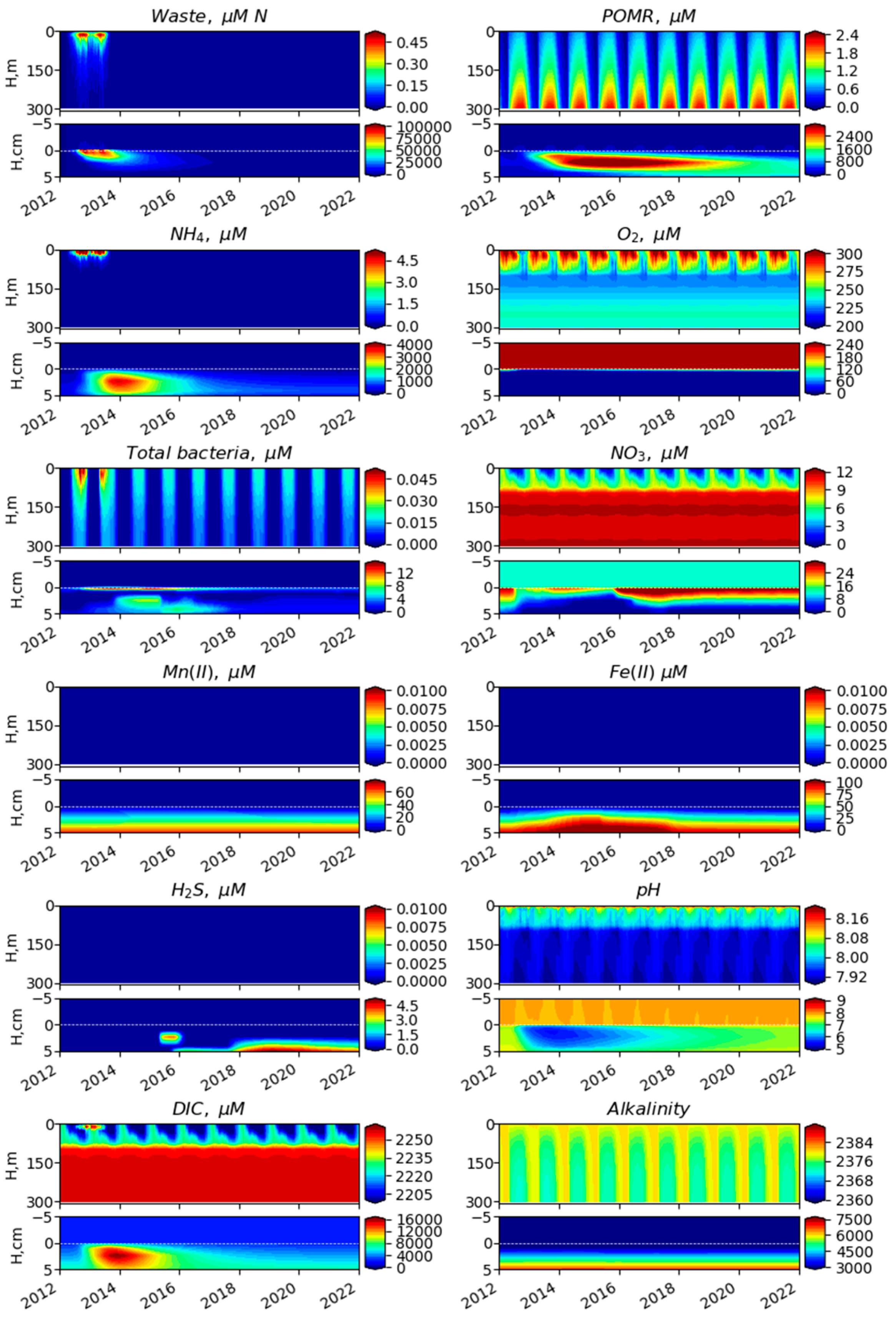
3.2. Simulated Temporal and Spatial Distributions

Figure 8 shows the temporal variability of selected biogeochemical variables during a two-year period with a typical fish farm emissions scenario (active feeding from April 1 of the first year, to November 1 of the following year, see Figure 3).

In regions far from the fish farms (Figure 8, left column), the model simulates seasonal variations in background water biogeochemistry that are broadly consistent with observed natural cycles in Hardangerfjord (i.e., in DB Copernicus MEMS database, used for the forcing). A phytoplankton bloom occurs in April, increasing the surface water concentrations of oxygen and particulate/dissolved OM. Sinking particulate OM leads to decreased oxygen at around 100 m depth and an accumulation of particles at the bottom. Between late spring and late autumn, remineralization processes enhance the DON and ammonium and suppress the dissolved oxygen concentrations, until winter mixing resets the system. During summer, the benthic boundary layer is enriched with dissolved and particulate organic matter. The sediments (below SWI) appear to be largely unaffected by the seasonal background variability.

At the fish farm (Figure 8, right column), emissions beginning in April lead to an accumulation of waste at the bottom that results in a decrease of oxygen penetration depth and appearance of high concentrations of particulate organic matter and ammonium. At a depth of the cage center, the model predicts increased ammonium and decreased oxygen concentrations (better seen in Figure 10).

The modeled transect through the fish farm (Figure 9) suggests that the farm’s influence can be detected up to 1000 m from the cages at a depth of 250 m. Tidal currents can spread waste in all directions, but the largest influence is predicted exactly below the farm. This region is characterized by an accumulation of waste, increased dissolved/particulate organic matter and inorganic nutrients, and reduced oxygen penetration depth and pH.

Figure 10 shows the simulated temporal and spatial variability of waste, oxygen (O₂), ammonium (NH₄), phytoplankton (Phy), pH, and aragonite saturation (Ω_Ar) at 10 m depth in the water column. Depending on the direction of the current, fish farm waste can be detected up to 100 m from the farm. This water is enriched with ammonium, well beyond the range of seasonal variability. The model also predicts detectable local changes at 10 m depth in oxygen and phytoplankton (eutrophication) and in pH and aragonite saturation state (acidification), although these are small relative to seasonal variations.

Spatiotemporal variability in the first model layer above the seabed (1 mm above the SWI) is shown in Figure 11. Waste accumulates at up to 500 m distance from the farm and can be clearly detected during the farm’s operation (2012–2014) and up to four years after cessation of farm activity. Waste decomposition leads to oxygen depletion (reaching 0 µM), increased ammonium, and the appearance of reduced forms of Mn, Fe and H₂S, due to intensive mineralization of organic matter with changing electron acceptors. These impacts are longer-lasting, with oxygen and Mn(II) showing significant perturbations up to eight years after the cessation of farming. These long-lasting effects are also seen in the whole suite of modeled electron acceptors exactly as would be theoretically expected. Decomposition also releases CO₂, leading to strong decreases in bottom-water pH (~1 unit) and aragonite saturation state (to undersaturated values Ω_Ar < 1) during farm operation.

Figure 12 shows time-depth variability in the water column and sediments at the fish farm location. Waste accumulation on the seabed during farm operation and the subsequent deepening and decomposition of waste in the sediments causes an increase in sedimentary particulate organic matter, manganese ion concentration, and pH that can be detected for at least 10 years. Full restoration of oxygen penetration depth and sedimentary nitrate content also requires at least 10 years (though less obvious in Figure 12). The model also predicts increased levels of sedimentary bacteria and hydrogen sulfide during this period.

4. Discussion

In this work we used the 2DBP-BROM model to investigate biogeochemical impacts of a single, hypothetical fish farm positioned in relatively deep water (300 m) with limited flushing and resuspension at depth, focusing on the spatiotemporal scales of impacts. Model results were compared with observations from Hardangerfjorden, Norway. Given the difficulties of comparing predictions from a generalized and spatially simplified simulation with measurements from a real fjord, there was considerable agreement between measurement and modeled profiles with regard to the differences between affected and unaffected locations, both in the water column and in the sediments (Figure 5 and Figure 6). Significant correlations between modeled and observed values in the water column were found for most parameters (except total alkalinity, likely due to the intensive rain prior to sampling). Biases were small (<35% of modeled mean values) for water column oxygen, phosphate, nitrate, alkalinity and DIC. Bias was relatively large for water column ammonium (observed values were ~500% higher than the model), but the values are still correlated with the model data, and there were no so large bias in the sediments.

In surface waters, the modeled fish farm caused locally elevated ammonium levels (within about 100 m of the farm) driven by excretion from fish and waste mineralization (Figure 8, Figure 9 and Figure 10 and Figure 12). In the bottom water, the fish farm emissions led to an accumulation of organic matter and reduced oxygen concentration and depth of penetration into the sediments within about 1000 m from the farm (Figure 6, Figure 8, Figure 9, Figure 11 and Figure 12). Oxygen depletion near the cages, as well as increases in organic matter content and inorganic nutrients, such as ammonium, can have negative effects on fish and stimulate the growth of bacteria inside the cages. These processes are likely to inhibit the legally required recovery of sediments during farm following periods and can lead to the accumulation of harmful chemicals, such as antibiotics [9,37]. In addition, enhanced inorganic nutrients, such as ammonium have the potential to impact the growth and health of farmed and wild fish in close association with the farm [38,39]. The model predicted that oxygen in the bottom water exactly below the cages would reach suboxic levels, approaching the legislation threshold of 5 mg/L [13], 2.5 mL/L for critical farms, [40,41]. The model also predicted severe acidification (pH decreases of ~1 unit) in the bottom water and sediments during the period of farm operation in first tens of meters from the farm, driven by the release of dissolved inorganic carbon during degradation of fish farm waste (Figure 11). We stress, however, that these impacts are only predicted for our hypothetical, low-dispersion scenario and are not intended to apply to any of the specific fish farms, as shown in Figure 4.

The model results show that seasonal inputs and changes are stronger than farm effects for many parameters, and that the pelagic system resets annually in many cases. The farm effects are in the sediments, and the legacy POM can impact sediment biogeochemistry with potential consequences for bottom water oxygen consumption for prolonged periods of time, and potentially over large spatial scales. The complexity of geochemical processes under different redox conditions identifies mechanisms of mineralization of the fish farm waste (i.e., from oxic mineralization to denitrification, Mn and Fe reduction and sulfate reduction) that can potentially mitigate or enhance responses to loading.

After the cessation of farming, the modeled oxygen and pH restored gradually back to the reference condition over a timescale of 4–8 years (Figure 11 and Figure 13), that is in agreement with the recovery period duration estimate with the observations [42]. This slow recovery, relative to the standard 6-month following period, and the general scheme of 1–2 years for chemical recovery presented in Reference [42], was in part due to the deep-water, low-dispersion deposition scenario, but also reflects the long timescales of biochemical remediation processes in the model. In this case, the bottleneck or main rate-limiting process might be the process of bio-irrigation, whereby benthic fauna (mostly worms and thalassinid shrimps) flush out their burrows with bottom water, thus acting to remediate the increase in porewater DIC caused by the respiration of the organic matter derived from the fish farm waste (Figure 12). Model sensitivity experiments show that, if the assumed bio-irrigation rate is increased or decreased within plausible bounds, the chemical restoration timescale is correspondingly decreased or increased (Figure 14), suggesting that bio-irrigation is a key uncertainty to be addressed in future observational and modeling efforts.

The other key uncertainties identified by Reference [18] also pertain to our model, namely, the representations of microbial degradation, bioturbation, and transport across the sediment-water interface. In BROM, there are four dynamical bacteria populations defined by aerobic vs. anaerobic environmental adaptation and heterotrophic vs. chemo-autotrophic feeding modes [22]. This gives BROM the potential to capture a more nuanced microbial response to organic loading, but also exposes uncertainties and knowledge gaps that must be confronted to develop predictive mechanistic models. For example, with increased loading from the fish farm waste (doubling of typical emission levels) the chemo-autotrophic bacterial population in BROM can be stimulated, such as to produce an over-compensation of porewater DIC and a temporary increase in pH above reference levels (Figure 14b). While we cannot point to observational support for this at present, this does suggest a potential complexity/nonlinearity in the response of sedimentary microbial degradation, and one that might be better constrained with regular biogeochemical observations in affected areas. Regarding bioturbation, in the present BROM model, this responds only to oxygen concentrations (decreasing in anoxic conditions); while, in reality, this may respond to changes in the benthic faunal community following organic loading and the colonization of fish farm sites by opportunistic species, with limited bioturbation potential [43] or with strong bioturbation and bio-irrigation effects [42,44,45,46]. Moreover, the transport of solutes across the SWI is in BROM parameterized as an extension of the internal bioturbation diffusivity (plus molecular diffusion). However, in reality it may also depend on bottom current speeds, sediment substrate type, porosity, and small-scale topography/roughness [18]. A further uncertainty concerns the representation of transport and circulation processes in the fjord. Realistic plume dispersion can be estimated with a 3D approach, but in a 3D model, it is practically impossible to predict changes in the sediments with vertical and horizontal dualization as in the 2DBP model used herein.

To address these uncertainties, we suggest first that there is a need for more regular sampling and reporting of measurements, at fish farm and control sites, of biogeochemical variables (nutrients, oxygen, carbonate system, pH, alkalinity, organic matter, biomasses of different faunal and bacterial groups). Such variables give objective and quantitative data that are not tied to any particular monitoring system, and that are essential for the development of predictive mechanistic models, which tend to operate in terms of elemental mass or molar concentrations, rather than indices or individual abundances (useful as these are for other purposes). Ideally, such measurements would form part of regular long-term monitoring systems rather than being limited to short-duration research projects. It is also likely that controlled laboratory experiments could be devised to assist the parameterization of diffusivities and exchange rates, e.g., across the sediment-water interface.

5. Conclusions

We developed a 2-dimensional transport-biogeochemical model (2DBP-BROM) to analyze the changes in the water column and sediment oxygen and nutrient regimes caused by fish farm emissions. The model describes in detail the processes of organic matter mineralization in oxygen-depleted conditions that are vitally important for assessing biogeochemical impacts (i.e., denitrification, metal reduction, sulfate reduction). The model produced profiles of oxygen, nutrients, and carbonate chemistry that were in reasonable agreement with observations from an expedition to multiple fish farm and control sites in Hardangerfjord, Norway—although further observations and modeling work are needed to rigorously define boundary conditions and to provide a strong test of the model. We showed how the model could be used to investigate critical levels of aquaculture-derived organic loading that can cause the formation of hypoxic and anoxic conditions in the bottom water. The 2DBP-BROM model is thus a promising tool for managing the impacts of aquaculture on local water quality and for assessing the carrying capacity of fjord water bodies. At present this model cannot be used for licensing, but this work is a step forward to develop a component of a system for licensing first of all regarding the biogeochemical processes occurring in the bottom layer.

References

1. Bostock, J.; McAndrew, B.; Richards, R.; Jauncey, K.; Telfer, T.; Lorenzen, K.; Little, D.; Ross, L.; Handisyde, N.; Gatward, I.; et al. Aquaculture: Global status and trends. Philos. Trans. R. Soc. B Biol. Sci. 2010, 365, 2897–2912. [Google Scholar] [CrossRef] [PubMed]
2. Bannister, R.J.; Johnsen, I.A.; Hansen, P.K.; Kutti, T.; Asplin, L. Near- and far-field dispersal modelling of organic waste from Atlantic salmon aquaculture in fjord systems. ICES J. Mar. Sci. 2016, 73, 2408–2419. [Google Scholar] [CrossRef] [Green Version]
3. Taranger, G.L.; Karlsen, Ø.; Bannister, R.J.; Glover, K.A.; Husa, V.; Karlsbakk, E.; Kvamme, B.O.; Boxaspen, K.K.; Bjørn, P.A.; Finstad, B.; et al. Risk assessment of the environmental impact of Norwegian Atlantic salmon farming. ICES J. Mar. Sci. 2015, 72, 997–1021. [Google Scholar] [CrossRef] [Green Version]
4. Det Kongelige Norske Videnskapers Selskab (DKNVS), Norges Tekniske Vitenskapsakademi (NTVA). Verdiskaping Basert pa Produktive hav i 2050. 2012. SINTEF Norway. Available online: https://www.sintef.no/globalassets/upload/fiskeri_og_havbruk/publikasjoner/verdiskaping-basert-pa-produktive-hav-i-2050.pdf (accessed on 25 August 2020). (In Norwegian).
5. Corner, R.A.; Brooker, A.J.; Telfer, T.C.; Ross, L.G. A fully integrated GIS-based model of particulate waste distribution from marine fish-cage sites. Aquaculture 2006, 258, 299–311. [Google Scholar] [CrossRef]
6. Findlay, R.H.; Watling, L.; Mayer, L.M. Environmental impact of salmon net-pen culture on marine benthic communities in Maine: A case study. Estuaries 1995, 18, 145–179. [Google Scholar] [CrossRef]
7. Holmer, M.; Duarte, C.M.; Heilskov, A.; Olesen, B.; Terrados, J. Biogeochemical conditions in sediments enriched by organic matter from net-pen fish farms in the Bolinao area, Philippines. Mar. Pollut. Bull. 2003, 46, 1470–1479. [Google Scholar] [CrossRef]
8. Macleod, C.K.; Crawford, C.M.; Moltschaniwskyj, N.A. Assessment of long term change in sediment condition after organic enrichment: Defining recovery. Mar. Pollut. Bull. 2004, 49, 79–88. [Google Scholar] [CrossRef]
9. Valdemarsen, T.; Bannister, R.J.; Hansen, P.K.; Holmer, M.; Ervik, A. Biogeochemical malfunctioning in sediments beneath a deep-water fish farm. Environ. Pollut. 2012, 170, 15–25. [Google Scholar] [CrossRef]
10. Samuelsen, O.B.; Lunestad, B.T.; Hannisdal, R.; Bannister, R.; Olsen, S.; Tjensvoll, T.; Farestveit, E.; Ervik, A. Distribution and persistence of the anti sea-lice drug teflubenzuron in wild fauna and sediments around a salmon farm, following a standard treatment. Sci. Total Environ. 2015, 508, 115–121. [Google Scholar] [CrossRef] [PubMed]
11. Sweetman, A.K.; Norling, K.; Gunderstad, C.; Haugland, B.T.; Dale, T. Benthic ecosystem functioning beneath fish farms in different hydrodynamic environments. Limnol. Oceanogr. 2014, 59, 1139–1151. [Google Scholar] [CrossRef]
12. Broch, O.J.; Daae, R.L.; Ellingsen, I.H.; Nepstad, R.; Bendiksen, E.A.; Reed, J.L.; Senneset, G. Spatiotemporal dispersal and deposition of fish farm wastes: A model study from central Norway. Front. Mar. Sci. 2017, 4. [Google Scholar] [CrossRef] [Green Version]
13. Stigebrandt, A. Carrying capacity: General principles of model construction. Aquac. Res. 2011, 42, 41–50. [Google Scholar] [CrossRef]
14. Pérez, O.M.; Telfer, T.C.; Beveridge, M.C.M.; Ross, L.G. Geographical Information Systems (GIS) as a simple tool to aid modelling of particulate waste distribution at marine fish cage sites. Estuar. Coast. Shelf Sci. 2002, 54, 761–768. [Google Scholar] [CrossRef] [Green Version]
15. Jusup, M.; Geček, S.; Legović, T. Impact of aquacultures on the marine ecosystem: Modelling benthic carbon loading over variable depth. Ecol. Modell. 2007, 200, 459–466. [Google Scholar] [CrossRef]
16. Brigolin, D.; Meccia, V.L.; Venier, C.; Tomassetti, P.; Porrello, S.; Pastres, R. Modelling biogeochemical fluxes across a Mediterranean fish cage farm. Aquac. Environ. Interact. 2014, 5, 71–88. [Google Scholar] [CrossRef] [Green Version]
17. Falconer, L.; Telfer, T.C.; Ross, L.G. Investigation of a novel approach for aquaculture site selection. J. Environ. Manag. 2016, 181, 791–804. [Google Scholar] [CrossRef] [PubMed] [Green Version]
18. Bravo, F.; Grant, J. Modelling sediment assimilative capacity and organic carbon degradation efficiency at marine fish farms. Aquac. Environ. Interact. 2018, 10, 309–328. [Google Scholar] [CrossRef] [Green Version]
19. Aure, J.; Stigebrandt, A. Quantitative estimates of the eutrophication effects of fish farming on fjords. Aquaculture 1990, 90, 135–156. [Google Scholar] [CrossRef]
20. Ferreira, J.G.; Hawkins, A.J.S.; Bricker, S.B. Management of productivity, environmental effects and profitability of shellfish aquaculture—The Farm Aquaculture Resource Management (FARM) model. Aquaculture 2007, 264, 160–174. [Google Scholar] [CrossRef]
21. Skogen, M.D.; Eknes, M.; Asplin, L.C.; Sandvik, A.D. Modelling the environmental effects of fish farming in a Norwegian fjord. Aquaculture 2009, 298, 70–75. [Google Scholar] [CrossRef]
22. Yakushev, E.V.; Protsenko, E.A.; Bruggeman, J.; Wallhead, P.; Pakhomova, S.V.; Yakubov, S.K.; Bellerby, R.G.J.; Couture, R.-M. Bottom RedOx Model (BROM v.1.1): A coupled benthic-pelagic model for simulation of water and sediment biogeochemistry. Geosci. Model Dev. 2017, 10, 453–482. [Google Scholar] [CrossRef] [Green Version]
23. Griffiths, J.R.; Kadin, M.; Nascimento, F.J.A.; Tamelander, T.; Törnroos, A.; Bonaglia, S.; Bonsdorff, E.; Brüchert, V.; Gårdmark, A.; Järnström, M.; et al. The importance of benthic-pelagic coupling for marine ecosystem functioning in a changing world. Glob. Chang. Biol. 2017, 23, 2179–2196. [Google Scholar] [CrossRef] [Green Version]
24. Bruggeman, J.; Bolding, K. A general framework for aquatic biogeochemical models. Environ. Model. Softw. 2014, 61, 249–265. [Google Scholar] [CrossRef] [Green Version]
25. Butenschön, M.; Clark, J.; Aldridge, J.N.; Allen, J.I.; Artioli, Y.; Blackford, J.; Bruggeman, J.; Cazenave, P.; Ciavatta, S.; Kay, S.; et al. ERSEM 15.06: A generic model for marine biogeochemistry and the ecosystem dynamics of the lower trophic levels. Geosci. Model Dev. Discuss. 2015, 8, 7063–7187. [Google Scholar] [CrossRef] [Green Version]
26. Vindenes, H.; Orvik, K.A.; Søiland, H.; Wehde, H. Analysis of tidal currents in the North Sea from shipboard acoustic Doppler current profiler data. Cont. Shelf Res. 2018, 162, 1–12. [Google Scholar] [CrossRef]
27. Yakushev, E.V.; Kuznetsov, I.S.; Podymov, O.I.; Burchard, H.; Neumann, T.; Pollehne, F. Modeling the influence of oxygenated inflows on the biogeochemical structure of the Gotland Sea, central Baltic Sea: Changes in the distribution of manganese. Comput. Geosci. 2011, 37, 398–409. [Google Scholar] [CrossRef]
28. Shchepetkin, A.F.; McWilliams, J.C. The regional oceanic modeling system (ROMS): A split-explicit, free-surface, topography-following-coordinate oceanic model. Ocean Model. 2005, 9, 347–404. [Google Scholar] [CrossRef]
29. Okubo, A. Remarks on the use of “diffusion diagrams” in modeling scale-dependent diffusion. Deep. Res. Oceanogr. Abstr. 1976, 23, 1213–1214. [Google Scholar] [CrossRef]
30. Hansen, P.K.; Pittman, K.; Ervik, A. Organic waste from marine fish farms—Effects on the seabed. Mar. Aquac. Environ. 1991, 22, 105–119. [Google Scholar]
31. Hall, P.; Anderson, L.; Holby, O.; Kollberg, S.; Samuelsson, M.-O. Chemical fluxes and mass balances in a marine fish cage farm. I Carbon. Mar. Ecol. Prog. Ser. 1990, 61, 61–73. [Google Scholar] [CrossRef]
32. Wang, X.; Olsen, L.M.; Reitan, K.I.; Olsen, Y. Discharge of nutrient wastes from salmon farms: Environmental effects, and potential for integrated multi-trophic aquaculture. Aquac. Environ. Interact. 2012, 2, 267–283. [Google Scholar] [CrossRef] [Green Version]
33. Grasshoff, K.; Kremling, K.; Ehrhardt, M. Methods of Seawater Analysis; Grasshoff, K., Kremling, K., Ehrhardt, M., Eds.; Wiley: Weinheim, Germany, 1999; ISBN 9783527295890. [Google Scholar]
34. Mintrop, L.; Pérez, F.F.; González-Dávila, M.; Santana-Casiano, J.M.; Körtzinger, A. Alkalinity determination by potentiometry: Intercalibration using three different methods. Ciencias Mar. 2000, 26, 23–37. [Google Scholar] [CrossRef] [Green Version]
35. Van Heuven, S.; Pierrot, D.; Rae, J.W.B.; Lewis, E.; Wallace, D.W.R. MATLAB Program Developed for CO2 System Calculations. ORNL/CDIAC-105b. Carbon Dioxide Information Analysis Center, Oak Ridge National Laboratory, US Department of Energy, Oak Ridge, Tennessee. 2011; p. 530. Available online: https://cdiac.ess-dive.lbl.gov/ftp/co2sys/CO2SYS_calc_MATLAB_v1.1/?C=N;O=A (accessed on 25 August 2020).
36. Lewis, E.; Wallace, D. Program Developed for CO2 System Calculations; Carbon Dioxide Information Analysis Center, CDIAC-105, Lockheed Martin Energy Research Corporation for the US Department of Energy: Oak Ridge, Tennessee. 1998; pp. 1–21. Available online: https://www.osti.gov/dataexplorer/biblio/dataset/1464255 (accessed on 25 August 2020).
37. Hargrave, B. Empirical relationships describing benthic impacts of salmon aquaculture. Aquac. Environ. Interact. 2010, 1, 33–46. [Google Scholar] [CrossRef] [Green Version]
38. Wilkie, M.P. Mechanisms of ammonia excretion across fish gills. Comp. Biochem. Physiol. Part A Physiol. 1997, 118, 39–50. [Google Scholar] [CrossRef]
39. Piedecausa, M.A.; Aguado-Giménez, F.; García-García, B.; Telfer, T.C. Total ammonia nitrogen leaching from feed pellets used in salmon aquaculture. J. Appl. Ichthyol. 2010, 26, 16–20. [Google Scholar] [CrossRef]
40. Dong, X.; Qin, J.; Zhang, X. Fish adaptation to oxygen variations in aquaculture from hypoxia to hyperoxia. J. Fish. Aquac. 2011, 2, 23–28. [Google Scholar]
41. Abo, K.; Yokoyama, H. Assimilative capacity of fish farm environments as determined by the benthic oxygen uptake rate: Studies using a numerical model. Bull. Fish. Res. Agen. 2007, 19, 79–87. [Google Scholar]
42. Keeley, N.B.; Forrest, B.M.; Macleod, C.K. Benthic recovery and re-impact responses from salmon farm enrichment: Implications for farm management. Aquaculture 2015, 435, 412–423. [Google Scholar] [CrossRef]
43. Wheatcroft, R.A.; Jumars, P.A.; Smith, C.R.; Nowell, A.R.M. A mechanistic view of the particulate biodiffusion coefficient: Step lengths, rest periods and transport directions. J. Mar. Res. 1990, 48, 177–207. [Google Scholar] [CrossRef]
44. Keeley, N.B.; Macleod, C.K.; Taylor, D.; Forrest, R. Comparison of three potential methods for accelerating seabed recovery beneath salmon farms. Aquaculture 2017, 479, 652–666. [Google Scholar] [CrossRef]
45. Keeley, N.; Valdemarsen, T.; Woodcock, S.; Holmer, M.; Husa, V.; Bannister, R. Resilience of dynamic coastal benthic ecosystems in response to large-scale finfish farming. Aquac. Environ. Interact. 2019, 11, 161–179. [Google Scholar] [CrossRef] [Green Version]
46. Keeley, N.; Valdemarsen, T.; Strohmeier, T.; Pochon, X.; Dahlgren, T.; Bannister, R. Mixed-habitat assimilation of organic waste in coastal environments—It’s all about synergy! Sci. Total Environ. 2020, 699, 134281. [Google Scholar] [CrossRef] [PubMed]
Figure 1. Schematic representation of the benthic redox model (BROM) biogeochemical processes considered and the model’ domain.
Water 12 02384 g001
Figure 2. Scheme of the 2-dimensional benthic-pelagic model (2DBP).
Water 12 02384 g002
Figure 3. Modeled fish farm emissions (blue line) in the form of Particulate Organic Carbon fluxes over a typical two-year production cycle, also showing the source data from 2 fish farms in Hardangerfjord over several production cycles (filled dots) and the monthly median values (open circles) to which the model curve was fitted.
Water 12 02384 g003
Figure 4. Position of stations during the cruise to the Hardangerfjord 25–26 August 2016.
Water 12 02384 g004
Figure 5. Observed vertical distributions of temperature (T), salinity (S), dissolved oxygen (O2), phosphate (PO4), silicate (Si), nitrate and nitrite (NO3), ammonia (NH4), dissolved organic carbon (DOC), dissolved organic nitrogen (DON), dissolved organic phosphorus (DOP), total alkalinity (Alk), dissolved inorganic carbon (DIC), partial pressure of CO2 (pCO2), and pH calculated as a function of Alk and TIC at Station 6 located about 1000 m from a fish farm (lines) and values in the sample collected at 10 m depth and 20 m horizontal distance from the farm at Station 7 (bold crosses).
Water 12 02384 g005
Figure 6. Modeled and observed vertical distribution of dissolved oxygen (a), phosphate (b), nitrate (c), ammonium (d), total alkalinity (e), and dissolved inorganic carbon (f), in the water column and porewater. Light blue circles show concentrations observed at 300–1000 m distance from a farm in the water column at stations 1–7. Red and yellow circles show sediment porewater concentrations observed at 100 and 500 m from a farm (stations 200 and 199, respectively). All samples were taken in August. Colored lines show the distributions of modeled concentrations in the time interval ±1 month relative to observations (bottom) for different distances from a farm: 100 m (red), 500 m (yellow), 1000 m (green), and 1500 m (blue).
Water 12 02384 g006
Figure 7. Modeled and measured distributions of particulate organic nitrogen and waste and observed POM (all in umol N/L) (a) and dissolved oxygen (b) in the bottom water and upper sediments. Colored lines show the distributions of modeled concentrations in the time interval ±1 month relative to observations during the first year of farm functioning for different distances from a farm: 100 m (red), 500 m (yellow), 900 m (green), and 1400 m (blue). Red and yellow circles show sediment porewater concentrations observed at 100 and 500 m from a farm (stations 200 and 199, respectively).
Water 12 02384 g007
Figure 8. Modeled variability of phytoplankton (Phy), particulate semi-labile organic matter (POMR), oxygen (O2), ammonium (NH4), waste, during a two-year period with a typical fish farm installation scenario (from April 1 of the first year, to November 1 of the second year) in the reference region (left) and at the fish farm installation (right).
Water 12 02384 g008
Figure 9. Modeled distributions of selected biogeochemical variables: Particulate semi-labile organic matter (POMR), dissolved semi-labile organic matter (DOMR), ammonium (NH4), waste, pH, dissolved inorganic carbon (DIC), oxygen (O2), nitrate (NO3), total bacteria, hydrogen sulfide (H2S), alkalinity (Alk), aragonite saturation (ΩAr) along a transect through the fish farm, 400 days after the onset of farming activities.
Water 12 02384 g009
Figure 10. Modeled temporal variability of waste, oxygen (O2), ammonium (NH4), phytoplankton (Phy), pH and aragonite saturation (ΩAr) at 10 m depth at a transect through the fish farm.
Water 12 02384 g010
Figure 11. Temporal variability of waste, oxygen (O2), ammonium (NH4), Manganese(II) (Mn(II)), Iron(II) (Fe(II)), hydrogen sulfide (H2S), pH and aragonite saturation (ΩAr), and total bacteria in the bottom layer at a transect through the fish farm.
Water 12 02384 g011
Figure 12. Temporal variability of the model parameters during the 10 years below the fish farm operated in first two years.
Water 12 02384 g012
Figure 13. Variability of pH below the fish farm in 1 cm above the bottom (a) and at the SWI (b) before, during and after the farm installation.
Water 12 02384 g013
Figure 14. Modeled temporal variability of O2, pH and H2S in the bottom layer at a transect through the fish farm in case of an absence of relaxation of waste: single waste run (a), double waste rate (b), single waste run without bio-irrigation (c).
Water 12 02384 g014