Estimating Suspended Sediment Concentrations from River Discharge Data for Reconstructing Gaps of Information of Long-Term Variability Studies


Abstract
1. Introduction
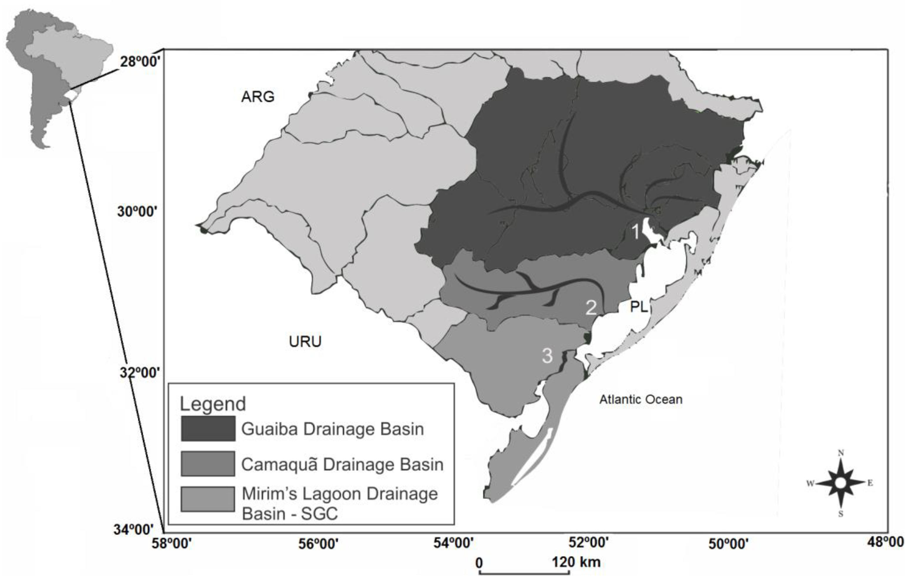
2. Study Area
3. Methods
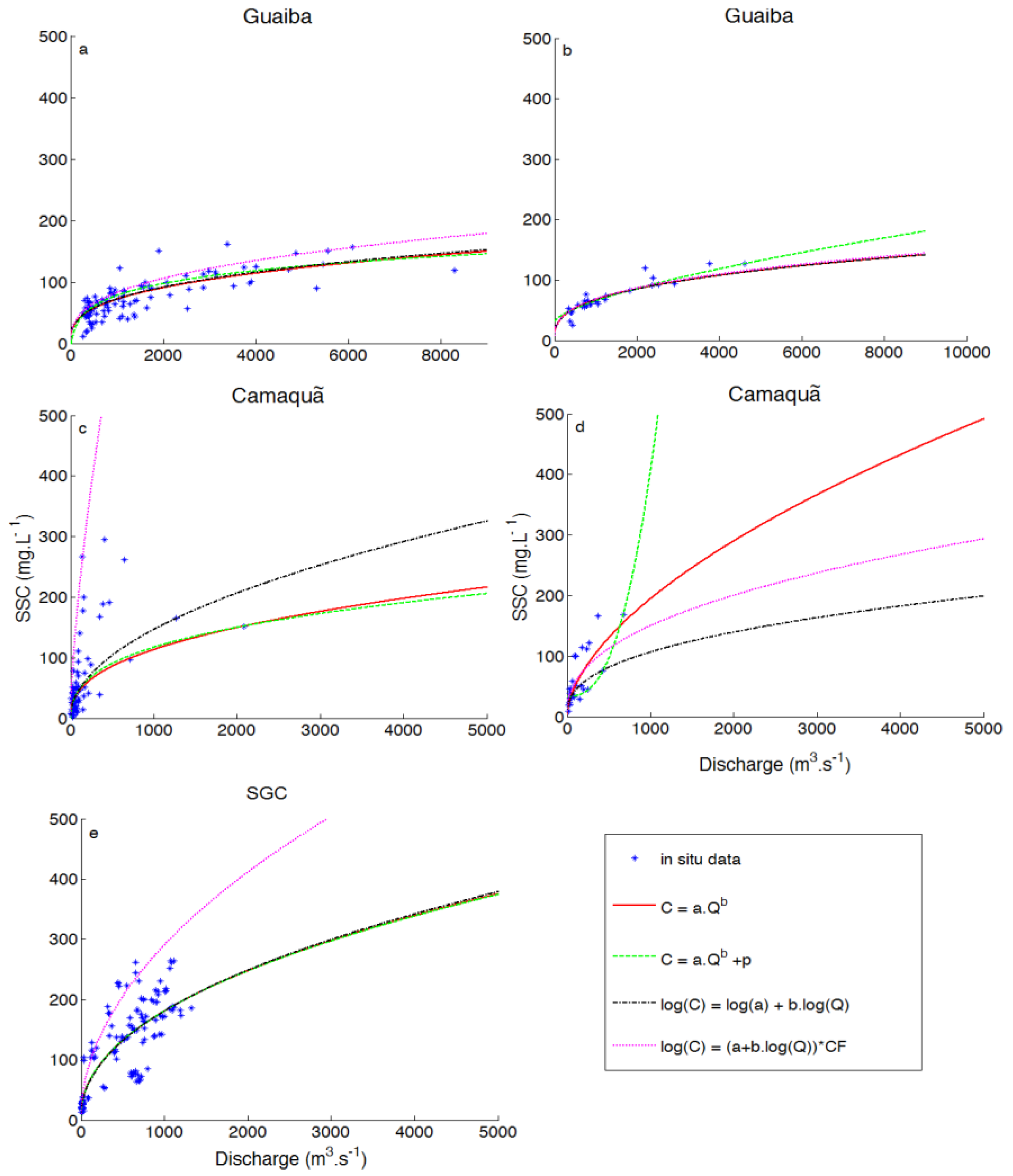
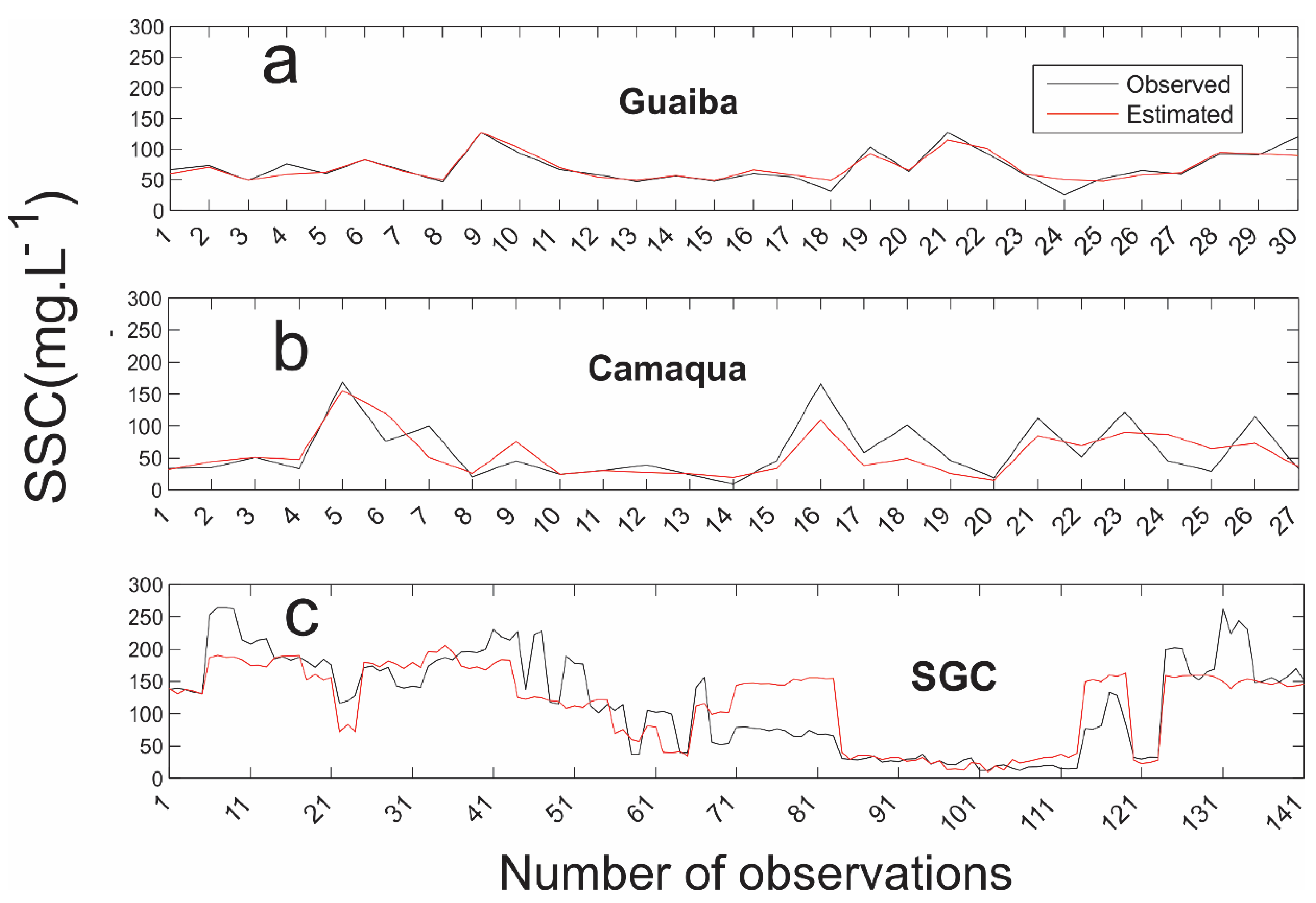
4. Results
5. Discussion
6. Conclusions
Author Contributions
Funding
Acknowledgments
Conflicts of Interest
References
- Toldo, E.E.; Dillenburg, S.; Corrêa, I.; Almeida, L.E.; Weschenfelder, J.; Gruber, N.L.S. Sedimentação de Longo e Curto Período na Lagoa dos Patos, Sul do Brasil. Pesqui. Geociênc. 2006, 33, 79–86. [Google Scholar] [CrossRef]
- Vieira, H.M.; Weschenfelder, J.; Fernandes, E.H.; Möller, O.O.; García-Rodríguez, F. Links between surface sediment composition, morphometry and hydrodynamics in a large shallow coastal lagoon. Sediment. Geol. 2020, 398, 105591. [Google Scholar] [CrossRef]
- Tanaka, H.; Lee, H.S. Influence of jetty construction on morphology and wave set-up at river mouth. Coast. Eng. 2003, 45, 659–683. [Google Scholar] [CrossRef]
- Bastos, L.; Bio, A.; Pinho, J.L.S.; Granja, H.; Jorge da Silva, A. Dynamics of the Douro estuary sand spit before and after breakwater construction. Estuar. Coast. Shelf Sci. 2012, 109, 53–69. [Google Scholar] [CrossRef]
- Garel, E.; Sousa, C.; Ferreira, O. Sand bypass and updrift beach evolution after jetty construction at an ebb-tidal delta. Estuar. Coast. Shelf Sci. 2015, 167, 4–13. [Google Scholar] [CrossRef]
- Lisboa, P.V.; Fernandes, E.H.L.; Espinoza, J.M.; Albuquerque, M.G. Variações Geomorfológicas do Pontal Sul do Estuário da Laguna dos Patos, RS. Brasil Sci. Plena 2015, 11, 1–6. [Google Scholar]
- Silva, P.D.; Lisboa, P.V.; Fernandes, E.H. Changes on the fine sediment dynamics after the Port of Rio Grande expansion. Adv. Geosci. 2015, 39, 123–127. [Google Scholar] [CrossRef]
- Prumm, M.; Iglesias, G. Impacts of port development on estuarine morphodynamics: Ribadeo (Spain). Ocean Coast. Manag. 2016, 130, 58–72. [Google Scholar] [CrossRef]
- Walling, D.E. Limitations of the rating curve technique for estimating suspended sediment loads, with particular reference to British rivers. In Erosion and Solid Matter Transport in Inland Waters; IAHS Publications: Wallingord, UK, 1977; pp. 34–48. [Google Scholar]
- Harrington, S.T.; Harrington, J.R. As assessment of the suspended sediment rating curve approach for load estimation on the Rivers Bandon and Owenabue, Ireland. Geomorphology 2013, 185, 27–38. [Google Scholar] [CrossRef]
- Zheng, M. A spatially invariant sediment rating curve and its temporal change following watershed management in the Chinese Loess Plateau. Sci. Total Environ. 2018, 630, 1453–1463. [Google Scholar] [CrossRef]
- Lai, C.; Chen, X.; Wang, Z.; Wu, X.; Zhao, S.; Wu, X.; Bai, W. Spatio-temporal variation in rainfall erosivity during 1960–2012 in the Pearl River Basin, China. Catena 2017, 137, 382–391. [Google Scholar] [CrossRef]
- Heng, S.; Suetsugi, T. Comparison of regionalization approaches in parameterizing sediment rating curve in ungauged catchments for subsequent instantaneous sediment yield prediction. J. Hydrol. 2014, 512, 240–253. [Google Scholar] [CrossRef]
- Barbetta, S.; Franchini, M.; Melone, F.; Moramarco, T. Enhancement and comprehensive evaluation of the rating curve model for different river sites. J. Hydrol. 2012, 464–465, 376–387. [Google Scholar] [CrossRef]
- Barbetta, S.; Moramarco, T.; Perumal, M. A Muskingum-based methodology for river discharge estimation and rating curve development under significant lateral inflow conditions. J. Hydrol. 2017, 554, 216–232. [Google Scholar] [CrossRef]
- Yang, G.; Chen, Z.; Yu, F.; Wang, Z.; Zhao, Y.; Wang, Z. Sediment rating parameters and their implications: Yangtze river, China. Geomorphology 2007, 85, 166–175. [Google Scholar] [CrossRef]
- Horowitz, A.J. A quarter century of declining suspended sediment fluxes in the Mississippi river and the e effect of the 1993 flood. Hydrol. Process. 2010, 24, 13–34. [Google Scholar] [CrossRef]
- Asselman, N. Fitting and interpretation of sediment rating curves. J. Hydrol. 2000, 234, 228–248. [Google Scholar] [CrossRef]
- Ferguson, R.I. River loads underestimated by rating curves. Water Resour. Res. 1986, 22, 74–76. [Google Scholar] [CrossRef]
- Kjerfve, B. Comparative Oceanography of Coastal Lagoons. In Estuarine Variability; Wolf, D.A., Ed.; Academic Press: New York, NY, USA, 1986; pp. 63–81. [Google Scholar]
- Calliari, L.J.; Winterwerp, J.C.; Fernandes, E.H.; Cuchiara, D.; Vinzon, S.B.; Sperle, M.; Holland, K.T. Fine grain sediment transport and deposition in the Patos Lagoon-Cassino beach sedimentary system. Cont. Shelf Res. 2009, 29, 515–529. [Google Scholar] [CrossRef]
- Vinzon, S.B.; Winterwerp, J.C.; Nogueira, R.; De Boer, G.J. Mud deposit formation on the open coast of the large Patos Lagoon-Cassino Beach system. Cont. Shelf Res. 2009, 29, 572–588. [Google Scholar] [CrossRef]
- Távora, J.; Fernandes, E.H.; Thomas, A.C.; Weatherbee, R.; Schettini, C.A. The influence of river discharge and wind on Patos Lagoon, Brazil, Suspended Particulate Matter. Int. J. Remote Sens. 2019, 40, 4506–4525. [Google Scholar] [CrossRef]
- Távora, J.; Fernandes, E.H.; Bitencourt, L.P.; Orozco, P. El Niño Southern Oscillation (ENSO) effects on the Variability of the Patos Lagoon Suspended Particulate Matter. Reg. Stud. Mar. Sci. 2020. submitted for publication. [Google Scholar]
- Bitencourt, L.P.; Fernandes, E.H.; Silva, P.; Möller, O.O. Spatio-temporal variability of suspended sediment concentrations on a shallow and turbid lagoon. Reg. Stud. Mar. Sci. 2020. submitted for publication. [Google Scholar]
- Marques, W.C.; Fernandes, E.H.; Monteiro, I.O.; Möller, O.O. Numerical modelling of the Patos Lagoon coastal plume, Brazil. Cont. Shelf. Res. 2009, 29, 556–571. [Google Scholar] [CrossRef]
- Marques, W.C.; Fernandes, E.H.; Moraes, B.C.; Möller, O.O.; Malcherek, A. Dynamics of the Patos Lagoon coastal plume and its contribution to the deposition pattern of the southern Brazilian inner shelf. J. Geophys Res. Oceans 2010, 115, 1–22. [Google Scholar] [CrossRef]
- Perez, L.; Crisci, C.; Hanebuth, T.J.J.; Lantzsch, H.; Perera, G.; Rodríguez, M.; Pérez, A.; Fornaro, L.; García-Rodríguez, F. Climatic oscillations modulating the Late Holocene fluvial discharge and terrigenous material supply of the Río de la Plata into the Southwestern Atlantic Ocean. J. Sed. Environ. 2018, 3, 205–219. [Google Scholar] [CrossRef]
- Möller, O.O.; Castaing, P.; Salomom, J.-C.; Lazure, P. The influence of local and non-local forcing effects on the subtidal circulation of Patos Lagoon. Estuaries 2001, 24, 297–311. [Google Scholar] [CrossRef]
- Marques, W.C.; Möller, O.O. Variabilidade temporal em longo período da descarga fluvial e níveis de água da Lagoa dos Patos, Rio Grande do Sul, Brasil. Rev. Bras. Rec. Híd. 2009, 13, 155–163. [Google Scholar] [CrossRef]
- Herz, R. Circulação das Águas de Superfície da Lagoa dos Patos. Ph.D. Thesis, Universidade de São Paulo, São Paulo, Brazil, 1977. [Google Scholar]
- Vaz, A.C.; Möller, O.O.; Almeida, T.L. Análise quantitativa da descarga dos rios afluentes da Lagoa dos Patos. Atlântida 2006, 28, 13–23. [Google Scholar]
- Ivanoff, M.D.; Toldo, E.E.; Figueira, R.C.L.; Ferreira, P.A.L. Use of 210Pb and 137Cs in the assessment of recent sedimentation in Patos Lagoon, Southern Brazil. Geo-Mar Lett. 2020. [Google Scholar] [CrossRef]
- Toldo, E.E. Sedimentação, Predição do Padrão de Ondas, e Dinâmica Sedimentar da Antepraia e Zona de Surfe do Sistema Lagunar. Ph.D. Thesis, Instituto de Geociências, Universidade Federal do Rio Grande do Sul, Porto Alegro, Brazil, 1994. [Google Scholar]
- Andrade Neto, J.S.D.; Rigon, L.T.; Toldo, E.E., Jr.; Schettini, C.A.F. Descarga sólida em suspensão do sistema fluvial do Guaíba, RS, e sua variabilidade temporal. Pesqui. Geociênc. 2012, 39, 161–171. [Google Scholar] [CrossRef]
- Bueno, C.; Figueira, R.; Ivanoff, M.D.; Toldo, E.; Fornaro, L.; García-Rodríguez, F. A multi proxy assessment of long-term anthropogenic impacts in Patos Lagoon, southern Brazil. J. Sed. Environ. 2019, 4, 276–290. [Google Scholar] [CrossRef]
- Dyer, K.R. Estuaries, 2nd ed.; Wiley: New York, NY, USA, 1997. [Google Scholar]
- Möller, O.O. Hydrodynamique de la Lagune dos Patos (30 RS, Brésil). Mesures et Modélisation. Ph.D. Thesis, University of Bordeaux I, Bordeaux, France, 1996. [Google Scholar]
- Fernandes, E.H.L.; Dyer, K.R.; Möller, O.O.; Niencheski, L.F.H. The Patos Lagoon Hydrodynamics during an El Niño event. Cont. Shelf Res. 2002, 22, 1699–1713. [Google Scholar] [CrossRef]
- Baisch, P. Les Oligo-Éléments Métalliques du Système Fluvio-Lagunaire dos Patos (Brésil)—Flux et Devenir. Ph.D. Thesis, University of Bordeaux I, Bordeaux, France, 1994. [Google Scholar]
- Oliveira, H.A.D.; Fernandes, E.H.; Möller, O.O.; Collares, G.L. Processos hidrológicos da Lagoa Mirim. Rev. Bras. Rec. Híd. 2015, 20, 34–45. [Google Scholar]
- Oliveira, H.A.D.; Fernandes, E.H.; Möller, O.O.; Garía-Rodriguez, F. Relationships between wind effect, hydrodynamics and water level in the world’s largest coastal lagoonal system. Water 2019, 11, 2209. [Google Scholar] [CrossRef]
- Hirata, F.E.; Möller, O.O.; Mata, M.M. Regime shifts, trends and interannual variations of water level in Mirim Lagoon, southern Brazil. Pan-Am. J. Aquat. Sci. 2010, 5, 254–266. [Google Scholar]
- Walling, D.E. Suspended sediment production and building activity in a small British Basin. In Effects of Man on the Interface of the Hydrological Cycle with the Physical Environment; IAHS Publication: Wallingford, UK, 1974; Volume 113, pp. 137–144. [Google Scholar]
- Walling, D.E. Assessing the accuracy of suspended sediment rating curves for a small basin. Water Resour. Res. 1977, 13, 531–538. [Google Scholar] [CrossRef]
- Syvitski, J.P.; Morehead, M.D.; Bahr, D.B.; Mulder, T. Estimating fluvial sediment transport: The rating parameters. Water Resour. Res. 2000, 36, 2747–2760. [Google Scholar] [CrossRef]
- Warrick, J.A.; Rubin, D. Suspended-Sediment Rating Curve Response To urbanization and wildfire, Santa Ana River, California. J. Geophys. Res. 2007, 112, F02018. [Google Scholar] [CrossRef]
- Higgins, A.; Restrepo, J.C.; Ortiz, J.C.; Pierini, J.; Otero, L. Suspended sediment transport in the Magdalena River (Colombia, South America): Hydrologic regime, rating parameters and effective discharge variability. Int. J. Sed. Res. 2016, 31, 25–35. [Google Scholar] [CrossRef]
- Warrick, J.A. Trend analyses with river sediment rating curves. Hydrol. Process. 2015, 29, 936–949. [Google Scholar] [CrossRef]
- Jha, B.; Jha, M.K. Rating Curve Estimation of Surface Water Quality Data Using LOADEST. J. Environ. Prot. Ecol. 2013, 4, 849–856. [Google Scholar] [CrossRef][Green Version]
- Horowitz, A.J. An evaluation of sediment rating curves for estimating suspended sediment concentrations for subsequent flux calculations. Hydrol. Process. 2003, 17, 3387–3409. [Google Scholar] [CrossRef]
- Crowder, D.; Demissie, M.; Markus, M. The accuracy of sediment loads when log-transformation produces nonlinear sediment load-discharge relationships. J. Hydrol. 2007, 336, 250–268. [Google Scholar] [CrossRef]
- Crawford, C.G. Estimation of suspended-sediment rating curves and mean suspended- sediment loads. J. Hydrol. 1991, 129, 331–348. [Google Scholar] [CrossRef]
- Cohn, T. Recent advances in statistical methods for the estimation of sediment and nutrient transport in rivers. Rev. Geophys. 1995, 33, 1117–1123. [Google Scholar] [CrossRef]
- Glysson, G.D. Sediment-Transport Curves; Technical Report 87 218; US Geological Survey: Reston, VI, USA, 1987.
- Moriasi, D.N.; Arnold, J.G.; Van Liew, M.W.; Bingner, R.L.; Harmel, R.D.; Veith, T.L. Model evaluation guidelines for systematic quantification of accuracy in watershed simulations. Trans. ASABE 2007, 50, 885–900. [Google Scholar] [CrossRef]
- Nash, J.E.; Sutcliffe, J.V. River flow forecasting through conceptual models part i|a discussion of principles. J. Hydrol. 1970, 10, 282–290. [Google Scholar] [CrossRef]
- Gupta, H.V.; Sorooshian, S.; Yapo, P.O. Status of automatic calibration for hydrologic models: Comparison with multilevel expert calibration. J. Hydrol. Eng. 1999, 4, 135–143. [Google Scholar] [CrossRef]
- Guo, Y.; Markus, M.; Demissie, M. Uncertainty of nitrate-n load computations for agricultural watersheds. Water Resour. Res. 2002, 38, 1185. [Google Scholar] [CrossRef]
- Chen, Z.; Li, J.; Shen, H.; Zhanghua, W. Yangtze river of china: Historical analysis of discharge variability and sediment flux. Geomorphology 2001, 41, 77–91. [Google Scholar] [CrossRef]
- Demissie, M.; Xia, R.; Keefer, L.; Bhowmik, N.G. Sediment budget of the Illinois river. Int. J. Sed. Res. 2003, 18, 305–313. [Google Scholar]
- EPA, U.S. Guidance for Quality Assurance Project Plans; Technical Report QA/G-5, EPA/240/R-02/009; United States Environmental Protection Agency: Washington, DC, USA, 2002.
- Colby, B. Relationship of Sediment Discharge to Stream Flow; Technical Report 56-27; US Department of the Interior, Geological Survey, Water Resources Division: Reston, VI, USA, 1956.
- Morlot, T.; Perret, C.; Favre, A.; Jalbert, J. Dynamic rating curve assessment for hydrometric stations and computation of the associated uncertainties: Quality and station management indicators. J. Hydrol. 2014, 517, 173–186. [Google Scholar] [CrossRef]
- Rovira, A.; Batalla, R.J. Temporal distribution of suspended sediment transport in a Mediterranean basin: The Lower Tordera (NE Spain). Geomorphology 2006, 79, 58–71. [Google Scholar] [CrossRef]
- Toldo, E.E.; Dillenburg, S.; Corrêa, I.; Almeida., L.E.; Weschenfelder, J. Sedimentação na Lagoa dos Patos e os Impactos Ambientais. In Proceedings of the Congresso da Associação Brasileira de Estudos do Quaternário, Guarapari, Brazil, 9–16 October 2005. [Google Scholar]


| RSR | NSE | PBIAS | |
|---|---|---|---|
| Very Good | 0 to 0.5 | 0.75 to 1.0 | <15 |
| Good | 0.5 to 0.6 | 0.65 to 0.75 | 10 to 30 |
| Satisfactory | 0.6 to 0.7 | 0.5 to 0.65 | 30 to 55 |
| Unsatisfactory | >0.7 | <0.5 | >55 |
| Normal | Log Based | |
|---|---|---|
| Guaíba—All Data | 0.76 | 0.77 |
| Guaíba—Monthly Average | 0.96 | 0.95 |
| Camaquã—All Data | 0.47 | 0.68 |
| Camaquã—Monthly Average | 0.87 | 0.84 |
| SGC—All Data | 0.80 | 0.89 |
| Coefficients | Calibration | Validation | ||||||||
|---|---|---|---|---|---|---|---|---|---|---|
| a | b | p | CF | RSR | NSE | PBIAS | RSR | NSE | PBIAS | |
| Guaíba—All data | ||||||||||
| Curve 1 | 7.09 | 0.34 | - | - | 0.60 | 0.64 | −1.49 | 0.60 | 0.64 | −2.56 |
| Curve 2 | 81.95 | 0.13 | −125 | - | 0.63 | 0.61 | −6.92 | 0.62 | 0.62 | −8.28 |
| Curve 3 | 0.84 | 0.34 | - | - | 0.60 | 0.64 | −2.20 | 0.60 | 0.65 | −3.28 |
| Curve 4 | 0.84 | 0.34 | - | 1.03 | 0.77 | 0.40 | −17.49 | - | - | - |
| Guaíba—Monthly Average | ||||||||||
| Curve 1 | 6.48 | 0.34 | - | - | 0.31 | 0.90 | 2.39 | 0.45 | 0.80 | 0.33 |
| Curve 2 | 0.36 | 0.66 | 30.17 | - | 0.29 | 0.92 | 1.72 | 0.41 | 0.83 | −0.50 |
| Curve 3 | 0.81 | 0.34 | - | - | 0.31 | 0.90 | 2.40 | 0.45 | 0.8- | 0.33 |
| Curve 4 | 0.81 | 0.34 | - | 1.00 | 0.30 | 0.91 | 0.69 | 0.44 | 0.80 | −1.40 |
| Camaquã—All data | ||||||||||
| Curve 1 | 7.00 | 0.40 | - | - | 0.85 | 0.27 | 25.14 | - | - | - |
| Curve 2 | 16.54 | 0.31 | 21.51 | - | 0.84 | 0.30 | 25.03 | - | - | - |
| Curve 3 | 0.68 | 0.50 | - | - | 0.83 | 0.31 | 19.24 | - | - | - |
| Curve 4 | 0.68 | 0.5 | - | 1.38 | 4.83 | 22.36 | 299.7 | - | - | - |
| Camaquã—Monthly Average | ||||||||||
| Curve 1 | 3.68 | 0.58 | - | - | 0.54 | 0.71 | −4.08 | 0.68 | 0.54 | 16.09 |
| Curve 2 | 8.3E-6 | 2.55 | 33.30 | - | 0.50 | 0.75 | 10.60 | 1.06 | −0.13 | 41.38 |
| Curve 3 | 0.86 | 0.39 | - | - | 0.70 | 0.52 | 18.73 | 0.89 | 0.20 | 32.90 |
| Curve 4 | 0.86 | 0.39 | - | 1.07 | 0.57 | 0.68 | −8.09 | 0.70 | 0.51 | 11.00 |
| São Gonçalo Channel—All data | ||||||||||
| Curve 1 | 7.88 | 0.45 | - | - | 0.58 | 0.66 | 0.87 | 0.60 | 0.65 | 4.38 |
| Curve 2 | 8.12 | 0.45 | 1.04 | - | 0.58 | 0.66 | 0.98 | 0.60 | 0.65 | 4.49 |
| Curve 3 | 0.88 | 0.46 | - | - | 0.58 | 0.66 | 1.28 | 0.60 | 0.64 | 4.81 |
| Curve 4 | 0.88 | 0.46 | - | 1.09 | 1.18 | −0.39 | −54.83 | - | - | - |
© 2020 by the authors. Licensee MDPI, Basel, Switzerland. This article is an open access article distributed under the terms and conditions of the Creative Commons Attribution (CC BY) license (http://creativecommons.org/licenses/by/4.0/).
Share and Cite
Jung, B.M.; Fernandes, E.H.; Möller, O.O., Jr.; García-Rodríguez, F. Estimating Suspended Sediment Concentrations from River Discharge Data for Reconstructing Gaps of Information of Long-Term Variability Studies. Water 2020, 12, 2382. https://doi.org/10.3390/w12092382
Jung BM, Fernandes EH, Möller OO Jr., García-Rodríguez F. Estimating Suspended Sediment Concentrations from River Discharge Data for Reconstructing Gaps of Information of Long-Term Variability Studies. Water. 2020; 12(9):2382. https://doi.org/10.3390/w12092382
Chicago/Turabian StyleJung, Bárbara M., Elisa H. Fernandes, Osmar O. Möller, Jr., and Felipe García-Rodríguez. 2020. "Estimating Suspended Sediment Concentrations from River Discharge Data for Reconstructing Gaps of Information of Long-Term Variability Studies" Water 12, no. 9: 2382. https://doi.org/10.3390/w12092382
APA StyleJung, B. M., Fernandes, E. H., Möller, O. O., Jr., & García-Rodríguez, F. (2020). Estimating Suspended Sediment Concentrations from River Discharge Data for Reconstructing Gaps of Information of Long-Term Variability Studies. Water, 12(9), 2382. https://doi.org/10.3390/w12092382