1. Introduction
The methodology for velocity estimation described in this paper pertains to the family of approaches for determining velocities in open-channel flows with the ultimate target for estimation of discharges. From this perspective, it is useful to call upon one of the classifications of these methods that categorize them as intrusive or nonintrusive approaches. Most of the conventional methods are intrusive, whereby probes, such as current meters, are submersed in the water column to acquire velocities at pre-established point locations. More recently, the advent of acoustic velocimetry has enabled us to acquire more efficient velocity measurements in the water column by simply placing the probes (such as an acoustic Doppler current profiler) in contact with the free surface [
1,
2]. Irrespective of their operating principle (e.g., mechanical, electrical or acoustic), probes that require submergence or contact with the water are associated with deployment of personnel and/or floating platforms (e.g., boats or instrument-attached rafts) in the stream, making their operation more complicated and at times even hazardous.
More recently, a plethora of nonintrusive instruments have been conceived and developed. These emerging instruments are based on acoustic, radar, laser and imagery principles for quantifying velocities at a point along a line or over a surface in the flow [
3,
4]. These instruments are emerging as instruments of choice, especially where personnel and equipment deployment are obstructed by adverse operating conditions (e.g., shallow or high turbulent waters; lack of access to the riverbanks). Image-based methods are among the most popular nonintrusive recently developed velocity and discharge measurement approaches being currently implemented under numerous configurations, and for a wide range of flow scales [
5,
6,
7].
The present paper introduces a new image-based method for estimating the velocity at a location at the free surface using an innovative approach that further simplifies operational concerns associated with other methods, making it cost-efficient compared with any other existing methods. While conventional image-based techniques track small and light particles suspended in the water column, or at the water free surface, under the assumption that they follow accurately the carrier flow [
8], the method proposed in this paper traces the changes in the wake shape generated by fixed objects piercing the free surface in open-channel flows as means of quantifying the channel velocity. The apparent shape of the wake velocity is an intricate physical process that can be explained under some well-defined conditions use linear water wave theory [
9]. Our approach is empirically based, whereby relationships between the wake angle and velocity of the channel flow are developed along with observations on critical dependencies in an effort to develop this method as an economic and rugged approach to measure velocity in streams. Although this method needs to make disturbances at the water surface, the velocimetry (camera) to acquire the wake images, and calculate the surface flow velocity, can be installed at a remote and safe place, reducing the risk of operational personnel and velocimetry damage during high-flow events.
The measurement methodology is explored with a series of flume experiments using a rod as the piercing object. The angle developing downstream of the object is captured with video recordings that are subsequently analyzed for determining the wake angle. Relationships are developed for each geometry of the piercing object and the kinematic characteristics of the flow are observed. The paper is organized as follows. The principle and the hypothesis associated with the methodology are presented first. The experimental setup is described next, followed by a description of the image analysis method applied to obtain the wake angle. The results of the experiments are then presented to reveal the relationships between angle and flow velocities for the tested cases. Finally, the conclusions on table flow conditions and applications of this method are presented.
2. Methodology Background
The principle of operation for the proposed velocity measurement method is based on tracing the shape of the wake produced by a floating or piercing object at the free surface of a moving body of water, such as a channel flow. While the piercing object can be stationary or moving, discussed in this paper are shapes created by slender stationary objects positioned at the top of the free surface. The V-shaped wake generated by the piercing object is familiar to many, as it resembles the free-surface pattern produced by, for example, a duck or a boat moving at the surface of a still, or a moving, body of water and the trace formed by a bridge pier downstream from its location. The wake of interest in the present context is defined as the lines passing through the highest peak of the waves that are formed on both sides of the object protruding from the free surface. While simple in appearance, the wake shape produces the results of quite an intricate wave-based interference process that has been extensively studied for generations. The free-surface pattern produced by such an object was first investigated in the 19th century when it was dubbed as the Kelvin wake [
10,
11,
12].
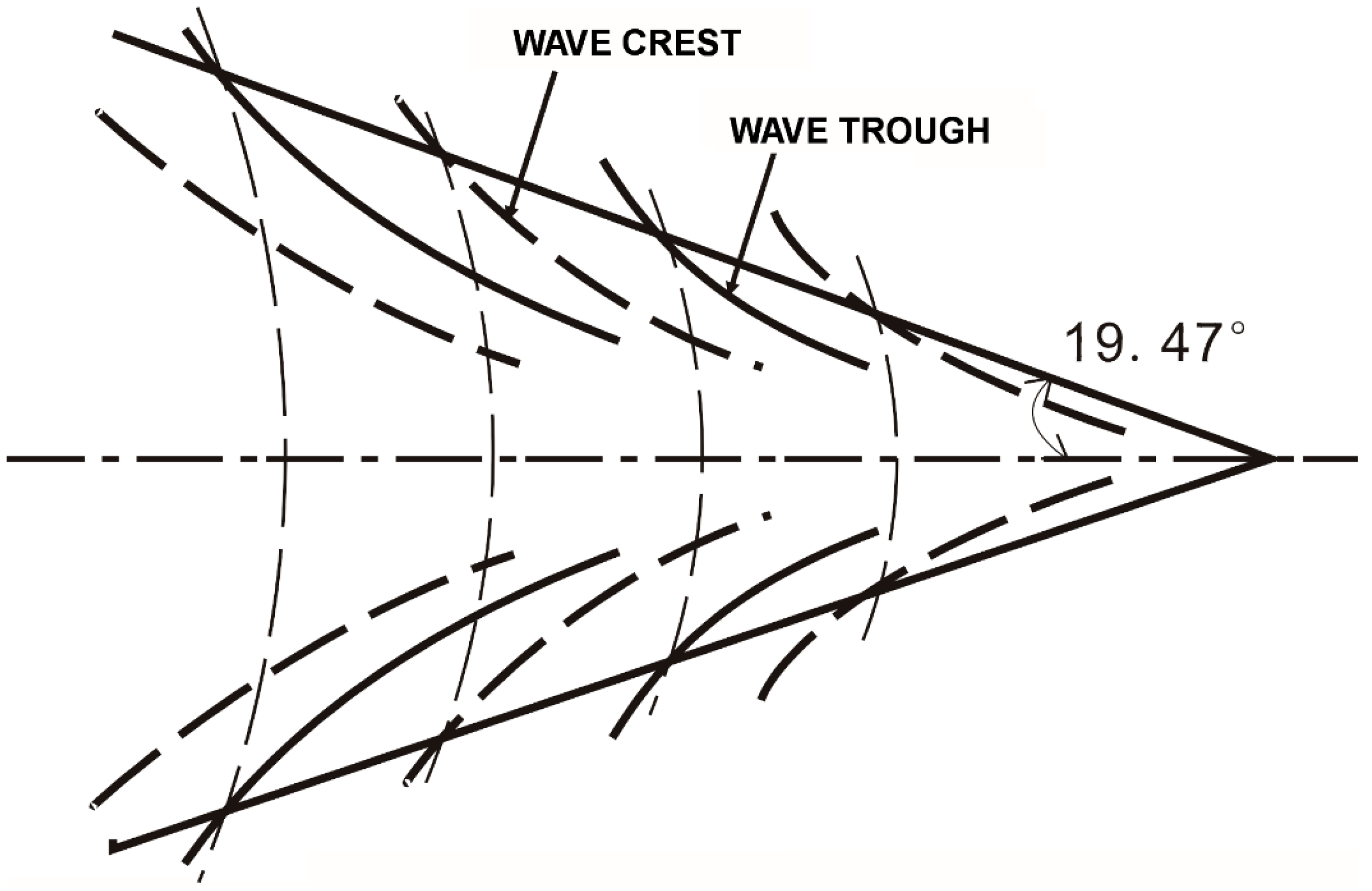
Kelvin wakes consist primarily of two components: divergent and transverse waves (see
Figure 1). Divergent waves are composed of a series of diagonal crests that look feathery in appearance and form two wake lines, which together form the cone or V shape. The second component, the transverse waves, move in arc and circular patterns in the area between the divergent waves. The half-angle of the wake makes an angle
of arcsin(1/3)
with respect to the direction of the moving object, and is independent of the moving object’s velocity or shape for an infinitely deep fluid [
11,
12,
13,
14]. This angle is labeled as the Kelvin angle in the present paper. However, many observations of wakes show this angle is variable depending on the water depth and the streamwise length of the object producing the disturbance [
9,
15,
16,
17,
18].
While the theoretical exploration of the wake generation is besides the scope of the present paper, we summarize here for completeness. The type of dependences of the wake’s half-angle,
, was documented with numerical simulations [
9]. Their findings are interpreted in the context of the wake produced by a fixed piercing object set at the surface of a moving water body and can be synthesized as follows:
- -
For infinitely deep water flow moving across a fixed object at a moderately velocity, is slightly less than the Kelvin angle.
- -
For infinitely deep flow moving across a fixed object at sufficiently high velocity, is further decreased with the inverse of the length-based Froude number. This body-length Froude is defined as where U is the mean flow velocity, g is the gravitational acceleration, and L is the length of the object in the streamwise direction.
- -
For a finite depth water layer moving across a fixed object,
increases from arcsin(1/3) to
as the depth-based Froude number
increases to 1, and then monotonically decreases for
> 1. The depth-based Froude number is defined as
, where
U is the mean flow velocity,
g is the gravitational acceleration and
h is the water depth [
19].
- -
For a moderately deep water layer moving across a fixed object, a different behavior of the angle from the finite-depth case is observed but quite similar with the infinite-depth case.
- -
For a shallow flow water layer, follow closely the Kelvin angle, becoming very large for moderately small numbers.
It is obvious from the above summary that some clear trends between the wake angle and velocity can be established for well-defined conditions of the two Froude numbers. Between these well-defined conditions, a transition zone exists where the dependencies are fuzzier. Moreover, the concepts of infinite and finite depths, as well as the conditions of shallow flow, carry themselves definitions that are not precisely captured by analytical formulations. For open channel flow in field conditions, the site conditions may bring in additional complexities such as boundary roughness effects that are not accounted for in these classifications, despite what might affect them. For the present context, we adopt a practical observational approach driven by the following hypothesis: the observed angle of the wake produced by a free-surface piercing object can be associated with the relative velocity between the flow and the object (see
Figure 2). In this study, we conducted experiments to obtain the empirically-observed relationship with the proper forms and dimensions of the piercing body and the different flow depths.
3. Experimental Setup
The laboratory study was conducted in 0.6 m-wide and 1.5 m-wide flumes with water recirculation capabilities and tailgate control to keep a constant water depth. The three-dimensional contraction shape, honeycombs and rocks were installed in the head-boxes for both flumes to maintain a steady flow condition in the measuring region. The 0.6 m-wide flume was 0.60 m wide, 10 m long and 0.3 m high. The experiments were carried out to quickly develop a relationship between the wake angles and the depth-based Froude number so as to guide the larger scale experiments. The 1.5 m-wide flume was 1.50 m wide, 19.50 m long and 2.13 m high. These experiments were close to the conditions in an actual stream at base flow and, therefore, acted as validation tests for the relationships observed in the small flume. Three types of metallic rods (round, square and rectangular) were tested having frontal widths of 0.95 cm in order to investigate the effects of the object shape and intrusiveness of the disturbance at the water surface (see
Table 1). The frontal width of 0.95 cm was large enough to produce a well-shaped wake downstream the object. The rectangular rod was tested in two different setting: one with the narrow edge (0.95 cm) set across the flow, and the other one with the wide edge (5.72 cm) set across the flow. The last test was aimed at testing the effect of the aspect ratio on the wake angle.
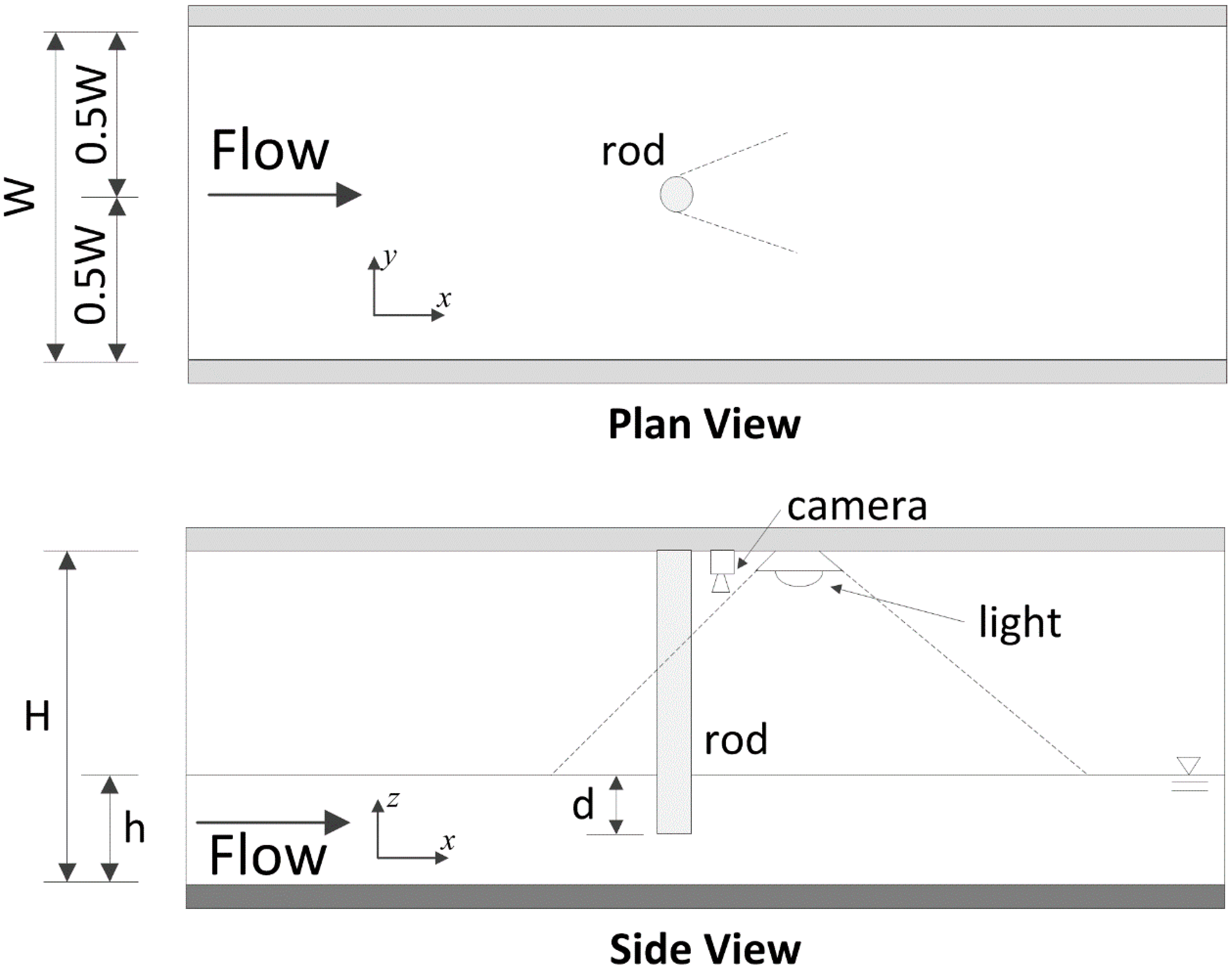
For all the small-scale facility experiments, the camera was mounted 60 cm above the flume perpendicular to the water surface. Two different water depths (30 cm and 10 cm) and variable velocities,
U (= flowrate/cross-section area) from 0.10 to 0.90 m/s, were used for the small-scale experiments. The observing region was in the middle length of the flume where the flow was steady. The rod was inserted into water from the free surface at the following distances: d = 1/30, 1/6, 1/2 and 1/1 of the water depth (
Figure 3). Experiments with the rod set at d = 1/30 were tested first then the rod was lowered to the next depth. For each set submergence, the flow velocities were varied sequentially at the pre-established values. Following the tests of one rod at all the submergence levels and velocities, another type of rod was installed and the experimental sequence described above was repeated.
The large-scale facility tests entailed round and square metallic rods with close aspect ratios, as summarized in
Table 1. All the tests from these series were conducted with the rod set firmly on the flume bottom. The rod length was sufficient to protrude through the water free surface for each tested case. The water depth was varied from 0.30 to 1.16 m, while the velocities ranged from 0.25 to 1.46 m/s. The video camera for acquiring the shape of the wake was mounted about 4 m above the open-channel free surface. Recording times between 30 and 60 s were taken for both the small- and large-scale experiments to provide a sufficient number of video fields for the postprocessing method described in the next section.
4. Image Analysis Method
The wake pattern developed downstream from the flow obstruction piercing the free surface is a flow area exposed to instabilities due to the inherent fluctuations of the turbulent structures triggered by the object piercing the free surface, as well as the effect of the large flow structures developing in the channel flow. To overcome the effect of these fluctuations, customized image processing software for automated conditioning and information extraction was created to enable accurate measurements of the wake angle α defined as the cone spanning between the stream-wise direction and the outer edge of the wake shape. The image postprocessing protocol was uniformly applied to all tested cases in the small and large-scale facility experiments. The outcome of the software was an enhanced view of the edges as a result of rotating the individual video frames to a reference position and applying averaging to the conditioned images. The obtained wake angle was related to the velocity of the underlying channel flow for each tested case.
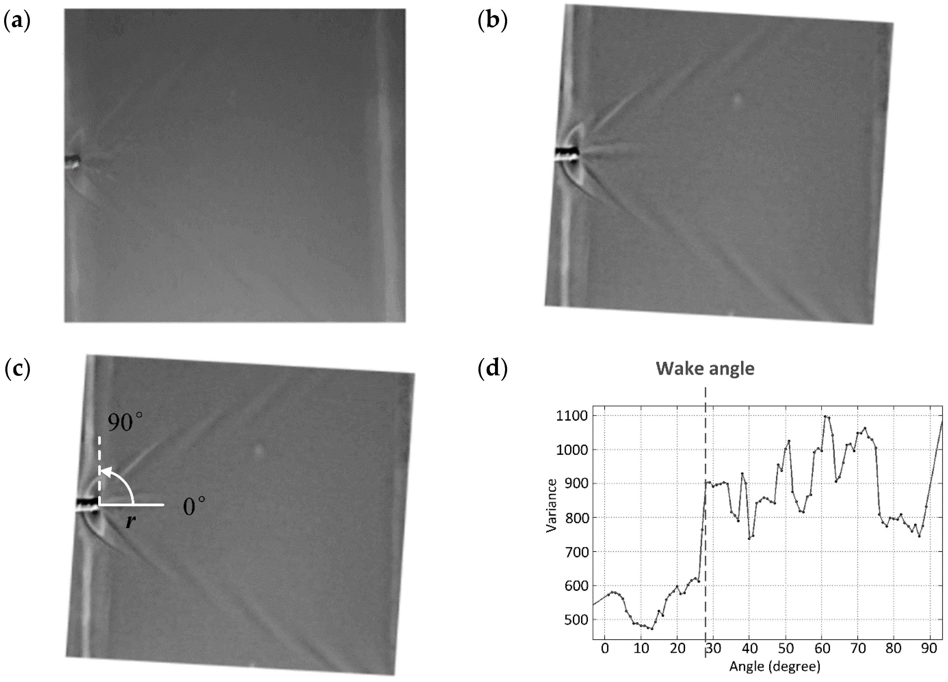
The sequence of steps of the image processing procedure is illustrated in
Figure 4. First, the successive images captured from the video-camera were transformed into gray-level images to strengthen the contrast of the wake shapes. At least 30 successive images as recorded with a video frequency of 30 frames per second (fps) were processed for each case. In the second step, the image preprocessing software applied procedures to overcome the effects of nonuniform illumination and wake rotation due to flow instability. For this purpose, the following tools available in the commercially-available software Matlab (
http://www.mathworks.com) were used: Sobel edge sharping, light compensation and correction for lens distortion. Then, the images were rotated to ensure that the wake direction in the image was aligned with the previous video field. The two steps of image processing described above are illustrated in
Figure 4a,b. They play the role of conditioning the raw images acquired during the experiments.
The third step of the customized image processing software process extracted the angle of the wake from the conditioned images. For this purpose, a fixed point on the rod was identified in the image and defined as the vertex of the wake. An automated search over the image was made to identify the edge of the wake. This scan was conducted within an appropriate radius (
r) and from 0 to 90 degree downstream of the vertex. Based upon visual inspection of the analyzed experiments, the scan radius (
r) was set between 50 and 100 pixel length. The actual length was set to be sufficient to make apparent the wake crest and trough associated with the wake patterns. The edge itself was identified based on the value of the pixel intensity variance,
, of the gray-level images within the scanned area. The variance of the pixel intensity along
r, can be expressed as:
where
n is the total number of points along
r,
g(
i) = gray levels intensity for each point along the path
I and
is the mean gray-level value for all points along the search radius,
r. The gray levels for each point were linearly interpolated from the gray values of adjacent pixels.
Visualization of image processing associated with the wake angle detection is provided in
Figure 4c,d.
Figure 4c visualizes the processing variables.
Figure 4d plots the variance of the image intensity over the scanned area at a given radius value from the vertex (i.e.,
r = 50 pixels). The figure displays an abrupt change in the variance. The first apparent peak of the variance indicates the significant change of the gray levels along
r, corresponding to the obvious appearance of the Kelvin wake (wave crest-trough patterns). In this study, we defined the first peak as the angle (
) of the Kelvin wake. We also assumed that the Kelvin wake is symmetrical along the horizontal line. Therefore, only the upper half plane in the image is scanned. Improper choice of the radius (
r) possibly affects the
values and subsequently the determination of the angle (
).
Figure 5 shows the radius (
r) against the
values. For a smaller
r, the obtained wake angle
shows significant fluctuations. As the chosen radius (
r) increases,
gradually approaches a constant value. For
r larger than 36 pixels, the wake angle tends to a constant value. Differences of about 0.38 degrees were observed, which can be regarded as the uncertainty on the wake angle. However, if the chosen
r is too small, the
value can be underestimated. Therefore, we recommend that initial visual inspection needs to be implemented to choose a proper scanning radius.
5. Results
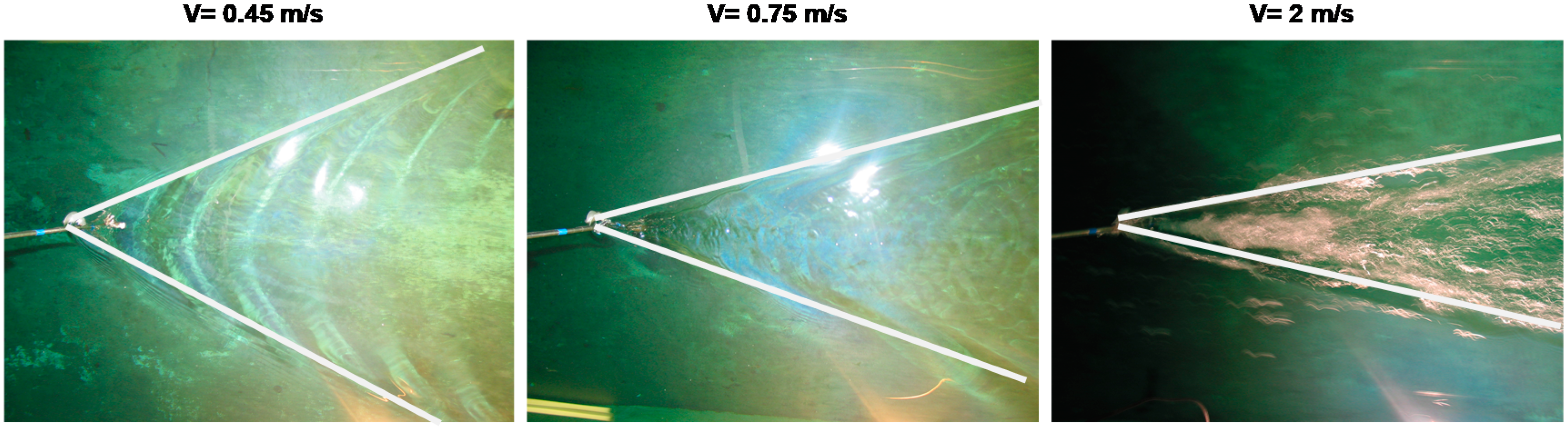
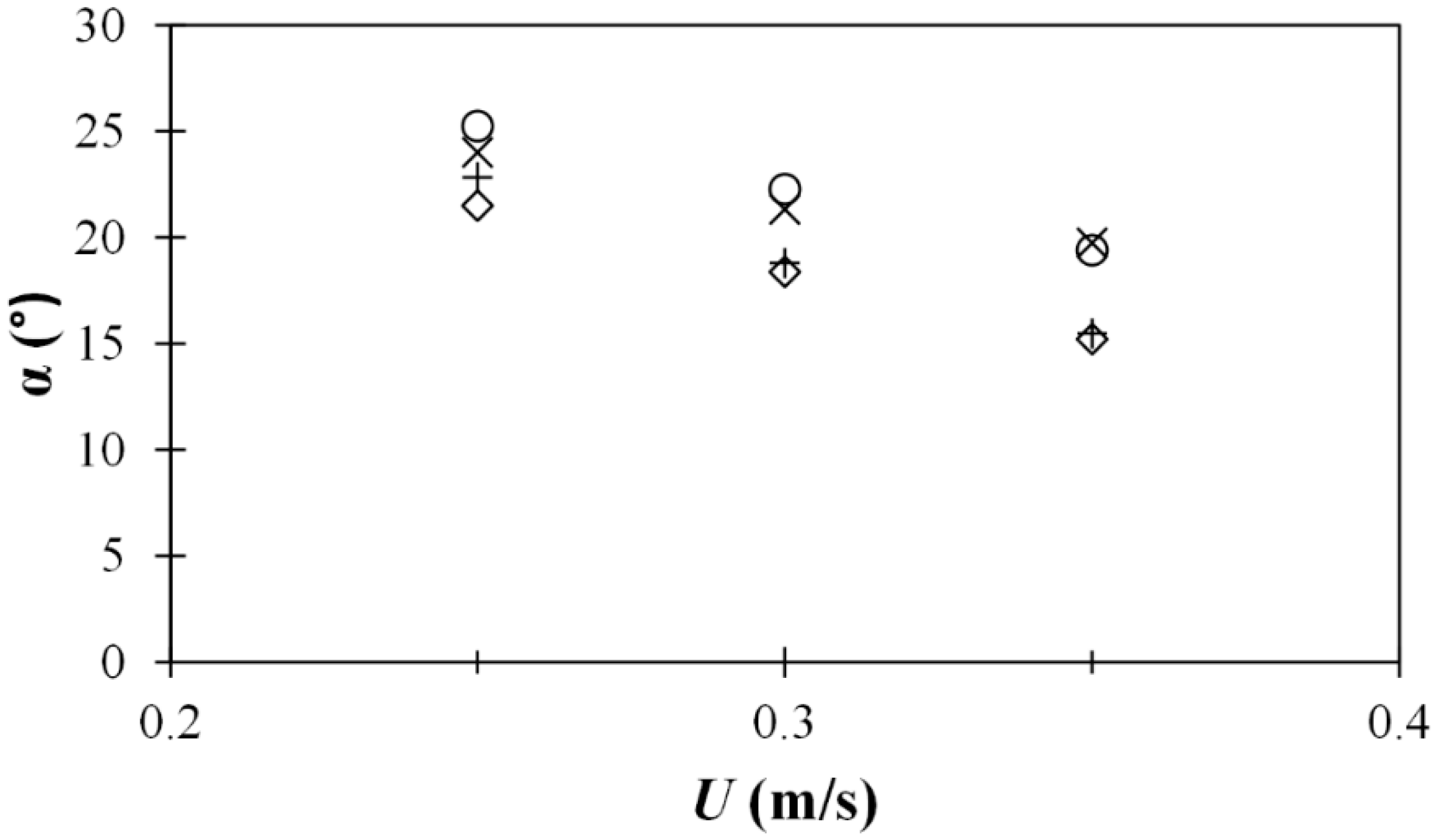
The effect of the submergence (d) of the rod on the wake angles was studied in a 0.6 m-wide flume (see
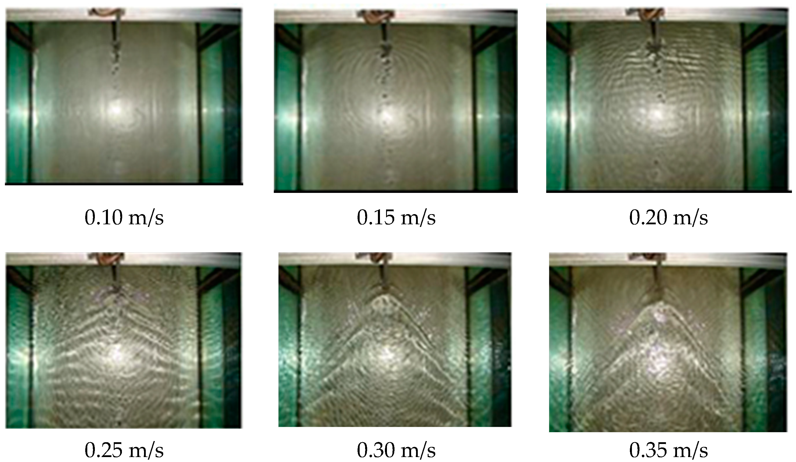
Figure 6).
Figure 7 shows the sequence of photos of flow across the round rod. From the experiments, it was found that the wake does not begin to form until the velocity is larger than 0.25 m/s, closely corresponding to the critical velocity (≈0.23 m/s) predicted by capillary-gravity wave theory [
20]. This is because the size (~0.95 cm) of the object placed in the water is comparable to the capillary length (
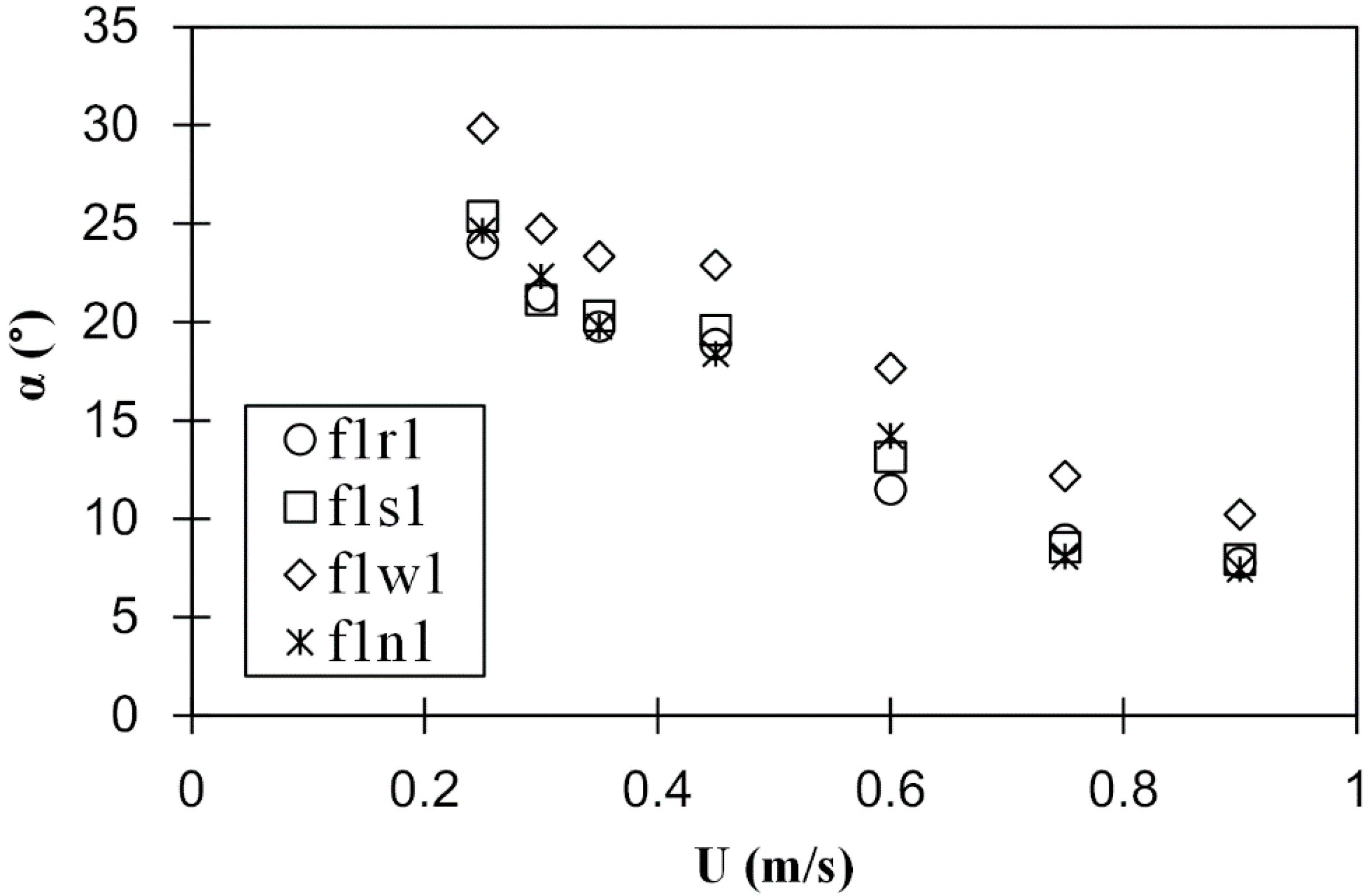
~0.3 cm for water at room temperature), and both capillary and gravitational forces affect the evolution of the wake patterns. When the velocity exceeds this value, the wake angle is greater than 19.47 degrees and tends to decrease with larger velocities. The angles for shallow penetration tend to be about four degrees narrower than the deeper penetration results. The accuracy of velocity measurements is limited when the penetration depth of the rod is not known, but the angles change in a predictable way when the depth is known. The four different shape probes have very similar angle with changing slope for all velocities. The wide edge rectangle followed the same slopes as the other three rod types but with a higher angle (about 5 degree) for these depths (see
Figure 8). The larger angles with the wide edge rod may be attributed to the fact that it has a too large frontal area for the flume. The rod may have functioned properly in the other much wider flume as it is expected that the wake area was affected by the flume walls. In addition, as Benzaquen et al., (2014) pointed out, the angle of the Kelvin wake is affected by the square root of the aspect ratio (the frontal width to the length along the flow direction) of the object [
21]. Therefore, the rectangular rod with a wide edge leads to a larger angle of the Kelvin wake than the rectangular rod with a narrow edge. This explains the slight differences due to the geometry of the object, which lead to an associated error of the wake angle of ~5 degree, i.e., ~0.1 m/s for different flow velocities. When the flow is larger, the relative error (difference between the measurements and actual value divided by the actual value) would reduce. The similarity of the relationship slopes for different rod shapes and penetration depths can be a more useful indicator for velocity measurements.
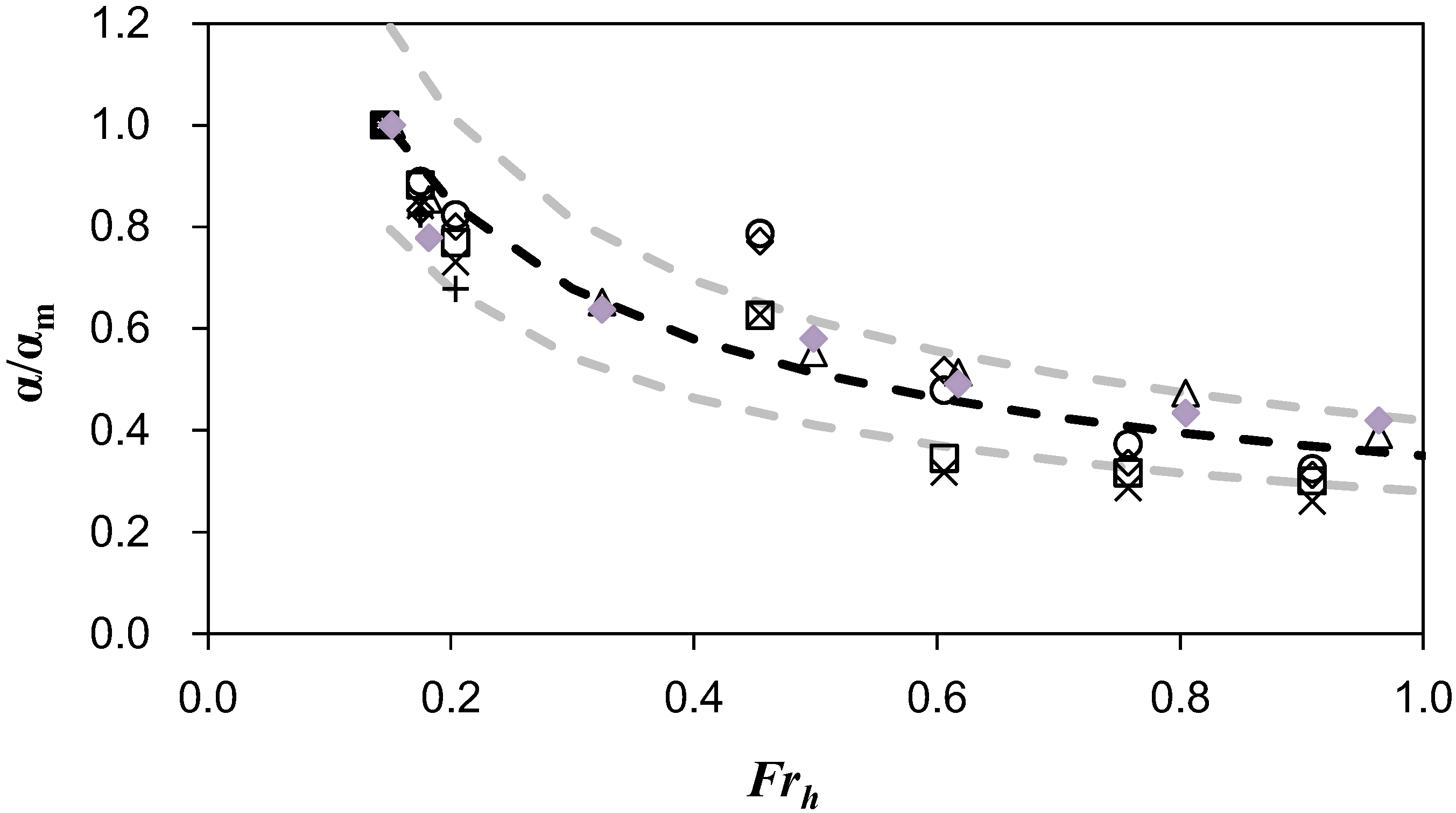
Similar results were obtained from the 1.5 m-wide flume. Six datasets with different geometry, intrusion depths of objects, and flume width, are shown in
Figure 9. The appearance of the wake angle velocity relationships can be improved by normalizing the angle with the maximum angle
of each dataset. The normalized angles are functions of the depth Froude number and can be expressed in two linear trend lines. For
< 0.6, the wake patterns are closer to the Kelvin wake. A V-shaped wake was formed by the transverse wave and diverging wave crests. For
> 0.6, the diverging wave is dominant and the V-shaped wake is formed by the diverging wave crests. Between the two linear trend lines, a gap around
≈ 0.55 can be found, which is approximately equal to the angle of 19 degrees in
Figure 8. This is because for low Froude numbers, the capillary wave and gravity wave are dependent on wake patterns. As the Froude number increases, (i.e., faster flows), the wake patterns are progressively controlled by the pure gravity wave. The transition between these two dominant mechanisms causes the instability of the wake pattern. At this instability region, it is difficult to determine the angle of the Kelvin wake. As the Froude number approaches 1.0, the angle formed by the diverging wave crest and the flow direction line is unsteady. It turns out that changes of wake angles are noticeable and measurable for a depth Froude number from 0.15 to 0.96 besides a small region around
≈ 0.55. This indicates that for subcritical flow conditions, the mean flow velocity can be easily calculated using the wake angle approach if the water depth is known. The linear fit parameters, related to the datasets used, may not be universal. For field applications, researchers or engineers still need to conduct field measurements to obtain the associated parameters.
6. Conclusions
The proposed image-based velocimetry method is simple, inexpensive and unobtrusive to flow. The laboratory experiments summarized in this paper illustrate that the Kelvin wake angle for a thin object piercing the free surface of a moving water stream decreases as the velocity increases for all depths. For the present experiments, the range of mean velocities varied between 0.10 and 0.90 m/s. This finding is confirmed for all rod shapes as well. It was determined that the shape of the thin rod piercing the free surface has no major effect on the Kelvin angle, irrespective of the water depth or velocity, as long as the frontal area is the same. Probes with exactly the same frontal area all provided very comparable results. The geometrical differences of objects lead to an associated error of ~5 degree in the wake angle, i.e., ~0.1 m/s for different mean flow velocities. When the flow is larger, the relative error (difference between the measurements and actual value divided by the actual value) would be less.
The proof-of-concept experiments reported above lead to the conclusion that the shape of the wake created by an object such as a boat, ship or bridge pier is usable to quantify velocities in subcritical flow conditions. For practical applications, the wake can be observed from a distance straight behind the object and a relative velocity can be calculated based on the wake angles. The authors deem that this method is low-cost and efficient to determine the relative velocity between an object set in the river and the flow of the stream for a range of flows. More comparative measurements are needed to assess the capabilities and limitations of the technique.


