Optimal Strategy to Tackle a 2D Numerical Analysis of Non-Uniform Flow over Artificial Dune Regions: A Comparison with Bibliography Experimental Results


Abstract
1. Introduction
2. Numerical Method
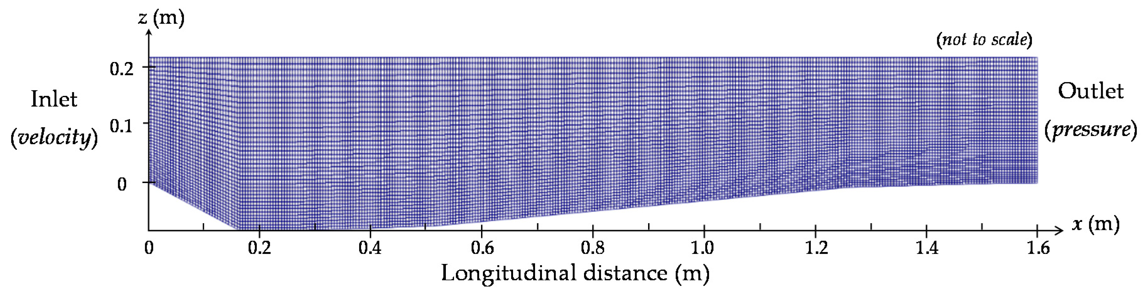
3. Model Setup
4. Results and Discussion
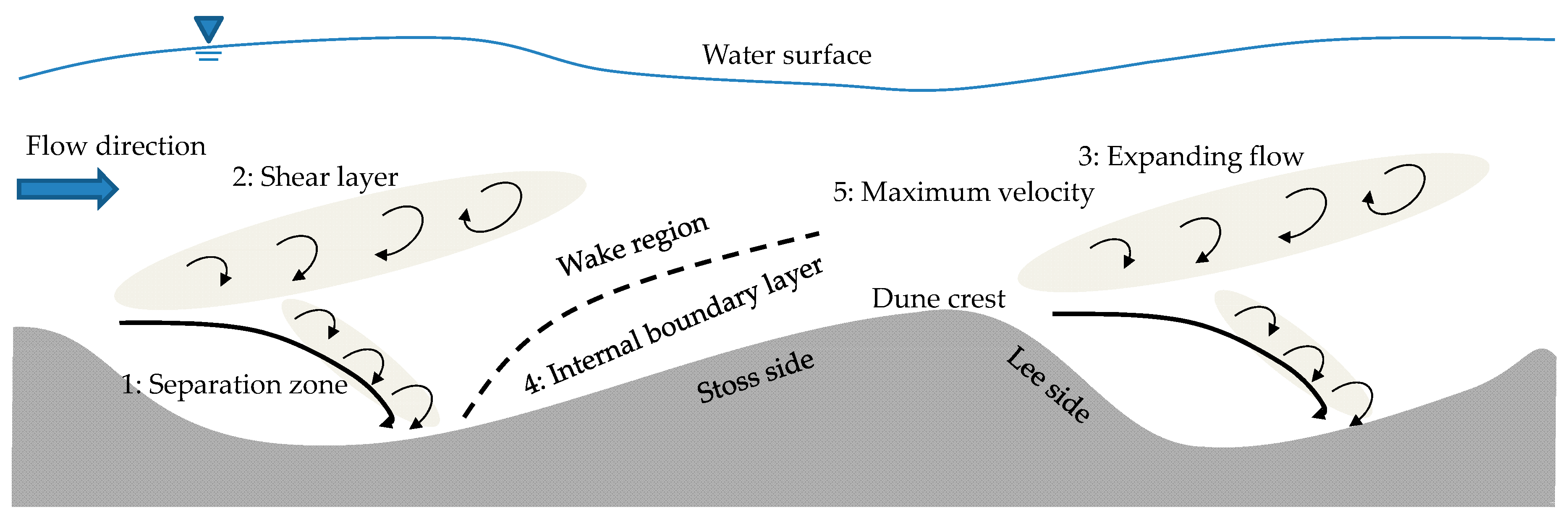
4.1. Flow Velocity and Turbulence Distribution
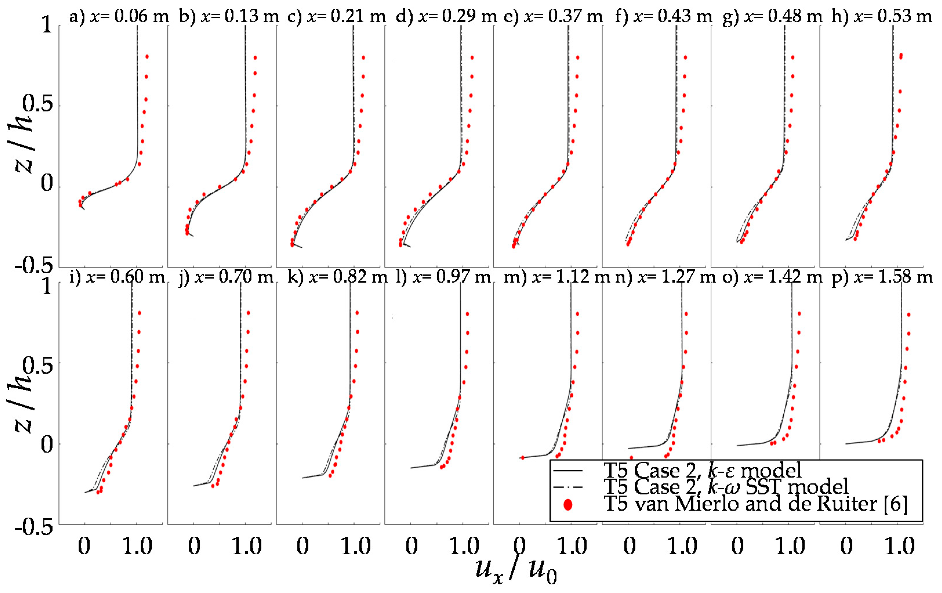
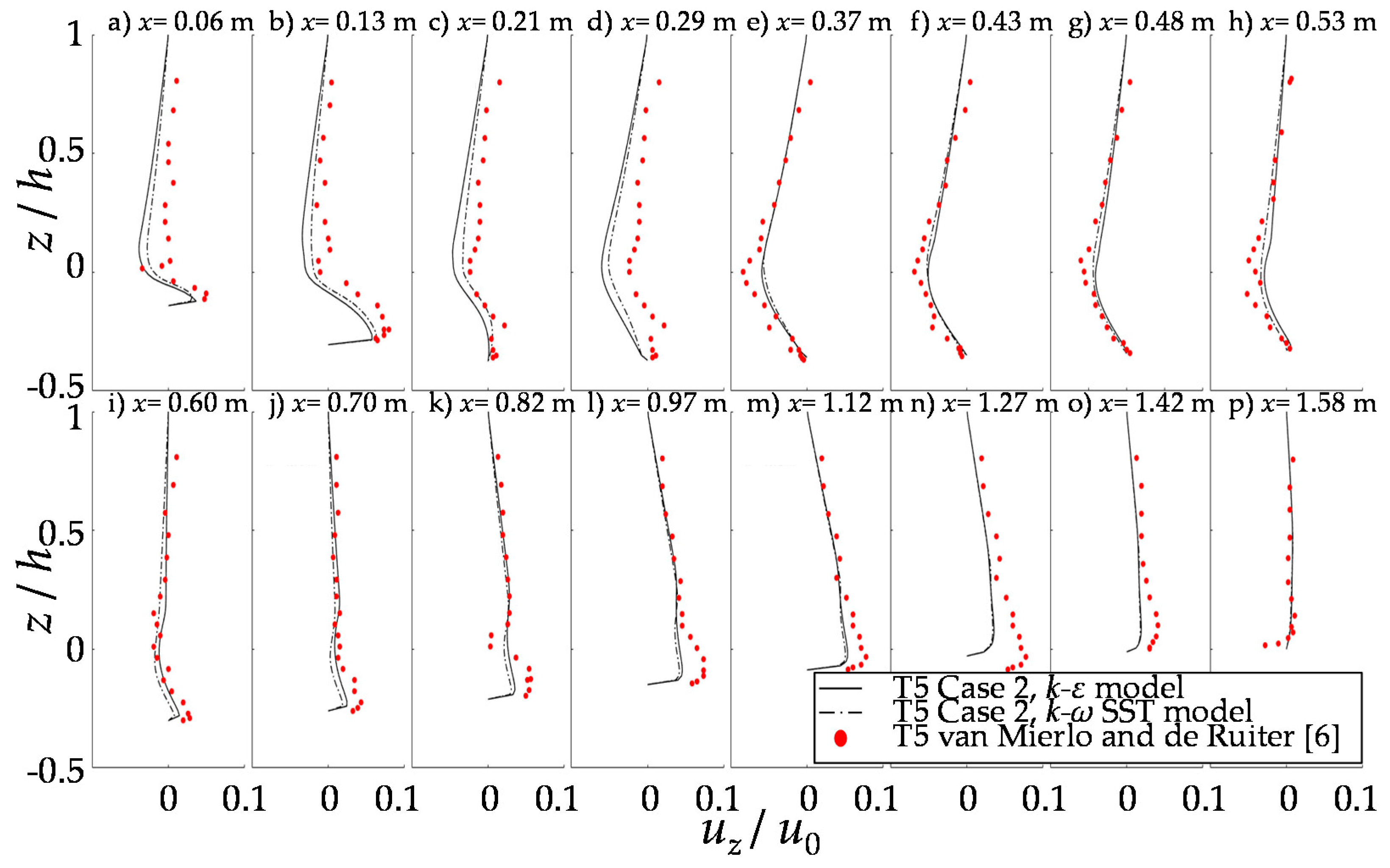
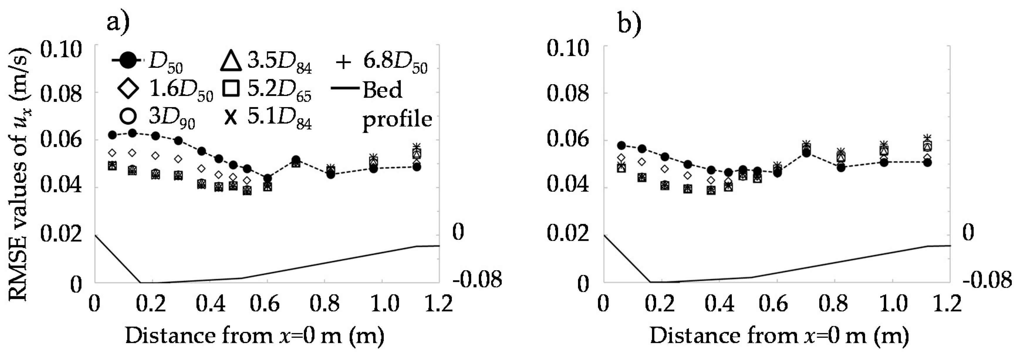
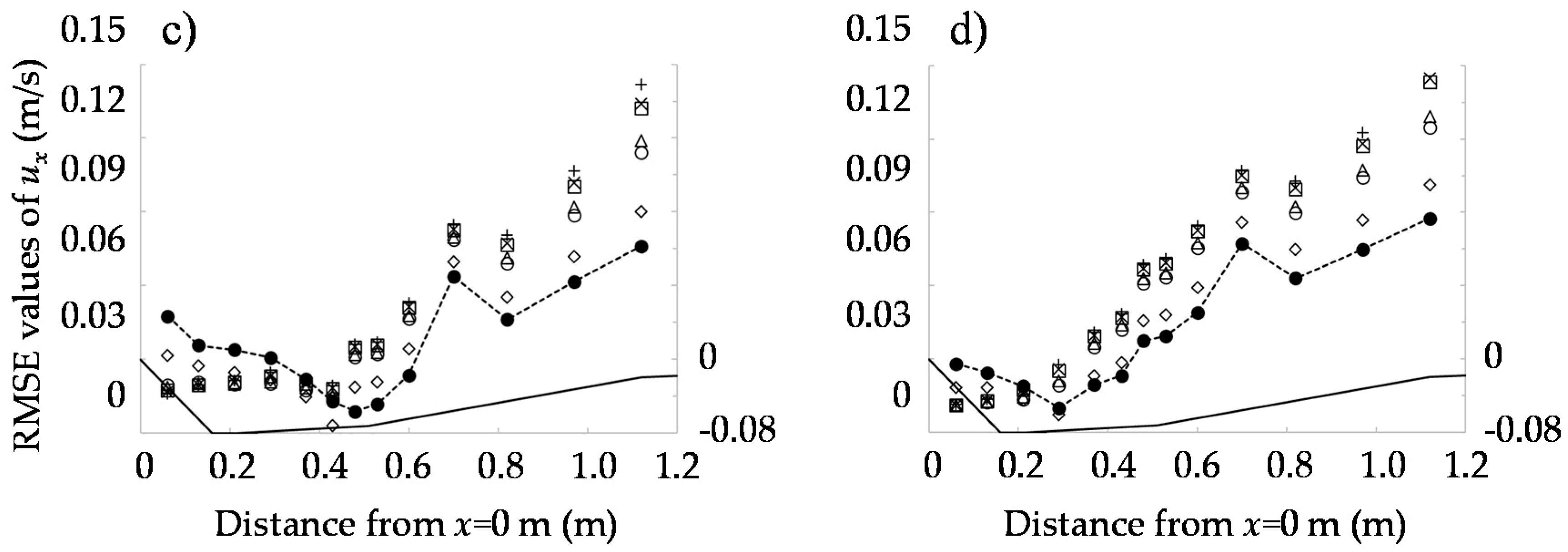
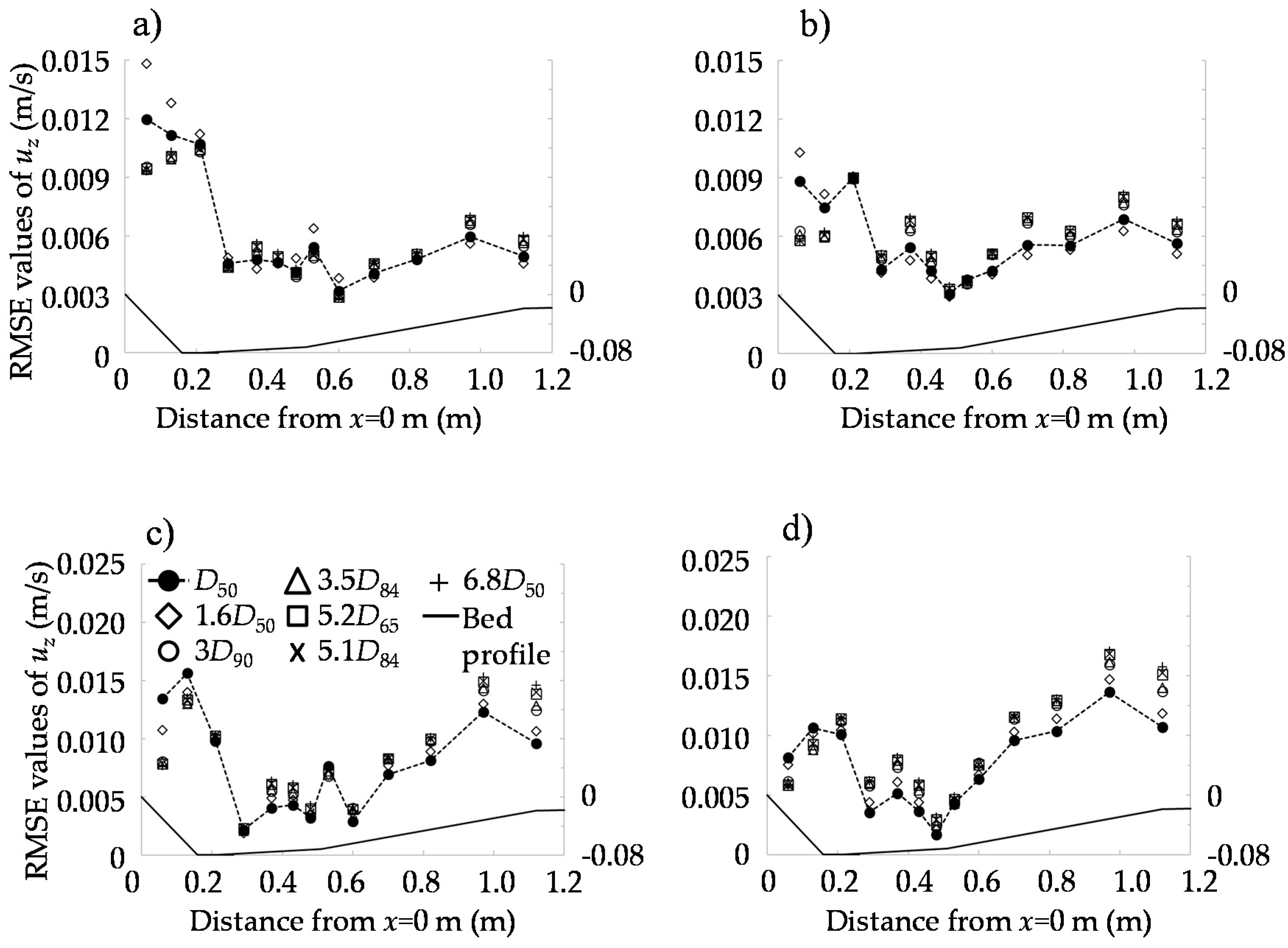
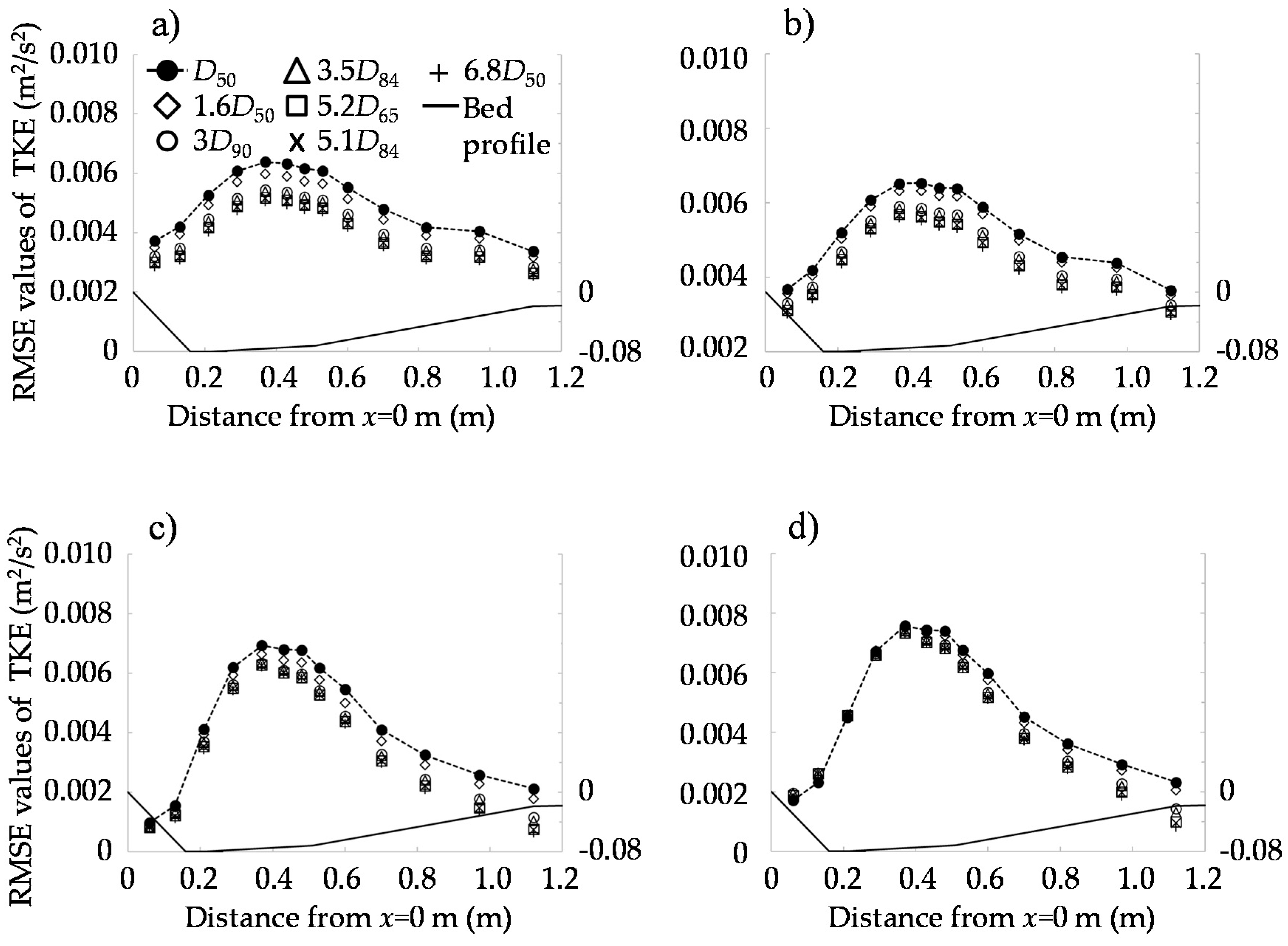
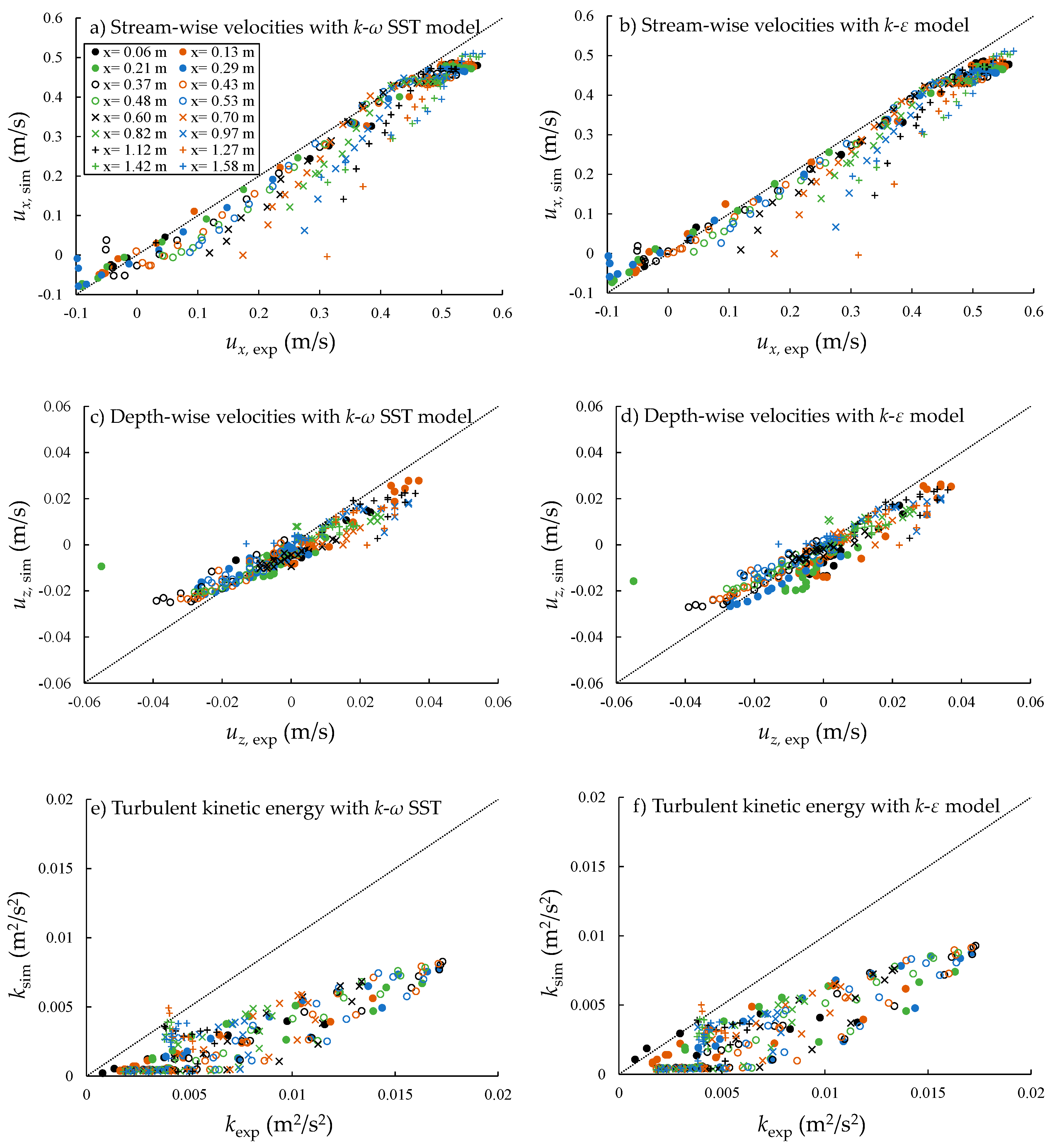
4.2. Comparison with Experiments
5. Summary and Conclusions
Author Contributions
Funding
Acknowledgments
Conflicts of Interest
Notations
| ,, | Model closure coefficients ( = 0.5532, = 0.4403, = 0.075, = 0.0828, = 0.8503, = 0.5, and = 0.8561) |
| Empirical constant (=0.09) | |
| , | Blending functions |
| Calibration coefficient (=0.31) | |
| Limited production function of the turbulent viscosity | |
| Diameter of particle intermediate axis for which n = 50%, 65%, 84%, and 90%, respectively, of the sample of bed material is finer | |
| Second blending function | |
| Dune height | |
| Inlet water depth | |
| Turbulent kinetic energy | |
| Roughness height | |
| Dune length | |
| Dune width | |
| Pressure | |
| Turbulent viscosity production | |
| Limited production term of the turbulent viscosity | |
| Absolute value of vorticity | |
| Flow velocities in stream-wise direction | |
| Flow velocities in water-depth direction | |
| Flow velocity at inlet | |
| Observed values (flow velocity and turbulent kinetic energy) from experiments in the previous research | |
| Calculated values (flow velocity and turbulent kinetic energy) from numerical modeling | |
| Velocity vector | |
| Stream-wise direction | |
| Depth-wise directional distance | |
| time | |
| Mesh size of first node from the wall | |
| Turbulent dissipation | |
| Kinematic viscosity coefficient | |
| Turbulent kinematic eddy viscosity coefficient | |
| Turbulent frequency (rate of dissipation of the eddies) | |
| Water temperature |
References
- Breusers, H.N.C. Time scale of two-dimensional local scour. In Proceedings of the 12th IAHR-Congress, Fort Collins, CO, USA, 11–14 September 1967; pp. 275–282. [Google Scholar]
- Hoffmans, G.J.C.M.; Booij, R. Two-dimensional modelling of local-scour holes. J. Hydraul. Res. 1993, 31, 615–634. [Google Scholar] [CrossRef]
- Park, S.W. Experimental Study of Local Scouring at the Downstream of River Bed Protection. Ph.D. Thesis, Seoul National University, Seoul, Korea, February 2016. [Google Scholar]
- Park, S.W.; Hwang, J.W.; Ahn, J. Physical modeling of spatial and temporal development of local scour at the downstream of bed protection for low Froude number. Water 2019, 11, 1041. [Google Scholar] [CrossRef]
- Ahn, J.; Yen, H. Semi-two dimensional numerical prediction of non-equilibrium sediment transport in reservoir using stream tubes and theory of minimum stream power. KSCE J. Civ. Eng. 2015, 19, 1922–1929. [Google Scholar] [CrossRef]
- van Mierlo, M.C.L.M.; de Ruiter, J.C.C. Turbulence Measurements above Artificial Dunes; Report No. Q789; Delft Hydraulic Laboratory: Delft, The Netherlands, 1988. [Google Scholar]
- Lyn, D.A. Turbulence measurements in open-channel flows over artificial bed forms. J. Hydraul. Eng. 1993, 119, 306–326. [Google Scholar] [CrossRef]
- Nelson, J.M.; Mclean, S.R.; Wolfe, S.R. Mean flow and turbulence fields over two-dimensional bed forms. Water Resour. Res. 1993, 29, 3935–3953. [Google Scholar] [CrossRef]
- Mclean, S.R.; Nelson, J.M.; Wolfe, S.R. Turbulence structure over two-dimensional bed forms: Implications for sediment transport. J. Geophys. Res. 1994, 99, 12729–12747. [Google Scholar] [CrossRef]
- Bennett, S.J.; Best, J.L. Mean flow and turbulence structure over fixed, two-dimensional dunes: Implications for sediment transport and bed form stability. Sedimentology 1995, 42, 491–513. [Google Scholar] [CrossRef]
- Coleman, S.E.; Melville, B.W. Initiation of bed forms on a flat sand bed. J. Hydraul. Eng. 1996, 122, 301–310. [Google Scholar] [CrossRef]
- Kadota, A.; Nezu, I. Three-dimensional structure of space-time correlation on coherent vortices generated behind dune crest. J. Hydraul. Res. 1999, 37, 59–80. [Google Scholar] [CrossRef]
- Maddux, T.B. Turbulent Open Channel Flow over Fixed Three-Dimensional Dune Shapes. Ph.D. Thesis, University of California, Santa Barbara, CA, USA, 2002. [Google Scholar]
- Kostaschuk, R.; Villard, P.; Best, J. Measuring velocity and shear stress over dunes with acoustic Doppler profiler. J. Hydraul. Eng. 2004, 130, 932–936. [Google Scholar] [CrossRef]
- Best, J. The fluid dynamics of river dunes: A review and some future research directions. J. Geophys. Res. 2005, 110, F04S02. [Google Scholar] [CrossRef]
- Best, J. Kinematics, topology and significance of dune-related macroturbulence: Some observations from the laboratory and field. Spec. Publs. Int. Ass. Sediment 2005, 35, 41–60. [Google Scholar] [CrossRef]
- Coleman, S.E.; Nikora, V.I. Fluvial dunes: Initiation, characterization, flow structure. Earth Surf. Process. Landf. 2011, 36, 39–57. [Google Scholar] [CrossRef]
- Lee, H.Y.; Hsieh, H.N. Numerical simulations of scour and deposition in a channel network. Int. J. Sediment Res. 2003, 18, 32–49. [Google Scholar]
- Nagata, N.; Hosoda, T.; Nakato, T.; Muramoto, Y. Three-dimensional numerical model for flow and bed deformation around river hydraulic structures. J. Hydraul. Eng. 2005, 131, 1074–1087. [Google Scholar] [CrossRef]
- Wu, C.L.; Chau, K.W. Mathematical model of water quality rehabilitation with rainwater utilization: A case study at Haigang. Int. J. Environ. Pollut. 2006, 28, 534–545. [Google Scholar] [CrossRef]
- Liu, X.; Garcia, M.H. Three-dimensional numerical model with free water surface and mesh deformation for local sediment scour. J. Waterw. Portcoastaland Ocean Eng. 2008, 134, 203–217. [Google Scholar] [CrossRef]
- Guven, A.; Gunal, M. Hybrid modelling for simulation of scour and flow patterns in laboratory flumes. Int. J. Numer. Methods Fluids 2010, 62, 291–312. [Google Scholar] [CrossRef]
- Nguyen, T.H.H.; Lee, J.; Park, S.W.; Ahn, J. Two-dimensional numerical analysis on the flow and turbulence structures in artificial dunes. KSCE J. Civ. Eng. 2018, 22, 4922–4929. [Google Scholar] [CrossRef]
- Kyrousi, F.; Leonardi, A.; Roman, F.; Armenio, V.; Zanello, F.; Zordan, J.; Juez, C.; Falcomer, L. Large eddy simulations of sediment entrainment induced by a lock-exchange gravity current. Adv. Water Resour. 2018, 114, 102–118. [Google Scholar] [CrossRef]
- Ouro, P.; Juez, C.; Franca, M. Drivers for mass and momentum exchange between the main channel and river bank lateral cavities. Adv. Water Resour. 2020, 137. [Google Scholar] [CrossRef]
- Pope, S.B. Turbulent Flows; Cambridge University Press: Cambridge, UK, 2000. [Google Scholar]
- Hirsch, C. Numerical Computation of Internal and External Flows: The Fundamentals of Computational Fluid Dynamics, 2nd ed.; Butterworth-Heinemann: Massachusetts, MA, USA, 2007. [Google Scholar]
- Bayon, A.; Valero, D.; García-Bartual, R.; Vallés-Morán, F.J.; López-Jiménez, P.A. Performance assessment of OpenFOAM and FLOW-3D in the numerical modeling of a low Reynolds number hydraulic jump. Environ. Model. Softw. 2016, 80, 322–335. [Google Scholar] [CrossRef]
- Spalart, P.R. Strategies for turbulence modelling and simulations. Int. J. Heat Fluid Flow 2000, 21, 252–263. [Google Scholar] [CrossRef]
- Mendoza, C.; Shen, H.W. Investigation of turbulent flow over dunes. J. Hydraul. Eng. 1990, 116, 459–477. [Google Scholar] [CrossRef]
- Johns, B.; Soulsby, R.L.; Xing, J. A comparison of numerical model experiments of free surface flow over topography with flume and field observations. J. Hydraul. Res. 1993, 31, 215–228. [Google Scholar] [CrossRef]
- Yoon, J.Y.; Patel, V.C. Numerical model of turbulent flow over sand dune. J. Hydraul. Eng. 1996, 122, 10–18. [Google Scholar] [CrossRef]
- Cheong, H.F.; Xue, H. Turbulence model for water flow over two-dimensional bedforms. J. Hydraul. Eng. 1997, 123, 402–409. [Google Scholar] [CrossRef]
- Tan, C.A.; Sinha, S.K.; Ettema, R. Ice-cover influence on near-field mixing in dune-bed channel: Numerical simulation. J. Cold Reg. Eng. 1999, 13, 1–20. [Google Scholar] [CrossRef]
- Dimas, A.A.; Fourniotis, N.T.; Vouros, A.P.; Demetracopoulos, A.C. Effect of bed dunes on spatial development of open channel flow. J. Hydraul. Res. 2008, 46, 802–813. [Google Scholar] [CrossRef]
- Fourniotis, N.T.; Toleris, N.E.; Dimas, A.A.; Demetracopoulos, A.C. Numerical computation of turbulence development in flow over sand dunes. In Advances in Water Resources and Hydraulic Engineering; Springer: Berlin/Heidelberg, Germany, 2009. [Google Scholar]
- Hoffmans, G.J.C.M.; Verheij, H.J. Scour Manual, 1st ed.; CRC Press/A.A Balkema: Rotterdam, The Nethelands, 1997. [Google Scholar] [CrossRef]
- Amoudry, L.O.; Liu, P.L.F. Two-dimensional, two phase granular sediment transport model with applications to scouring downstream of an apron. Coast. Eng. 2009, 56, 693–702. [Google Scholar] [CrossRef]
- Termini, D. Bed scouring downstream of hydraulic structures under steady flow conditions: Experimental analysis of space and time scales and implications for mathematical modeling. Catena 2011, 84, 125–135. [Google Scholar] [CrossRef]
- Nguyen, T.H.H.; Ahn, J.; Park, S.W. Numerical and physical investigation of the performance of turbulence modeling schemes around a scour hole downstream of a fixed bed protection. Water 2018, 10, 103. [Google Scholar] [CrossRef]
- Spalart, P.R.; Allmaras, S.R. A one-equation turbulence model for aerodynamic flows. In Proceedings of the 30th Aerospace Sciences Meeting and Exhibit (AIAA, 92–0439), Reno, NV, USA, 6 January 1992; p. 439. [Google Scholar] [CrossRef]
- Colebrook, C.F.; White, C.M. Experiments with fluid friction in roughened pipes. Proc. R. Soc. A Math. Phys. Eng. Sci. 1937, 161, 367–381. [Google Scholar] [CrossRef]
- Nelson, J.M.; Smith, J.D. Mechanics of flow over ripples and dunes. J. Geophys. Res. 1989, 94, 8146–8162. [Google Scholar] [CrossRef]
- Jellesma, M. Form Drag of Subaqueous Dune Configurations. Master’s Thesis, University of Twente, Enschede, The Netherlands, November 2013. [Google Scholar]
- van Rijn, L.C. Principles of Sediment Transport in Rivers, Estuaries, and Coastal Seas; Aqua Publications: Blokzijl, The Netherlands, 1993. [Google Scholar]
- McLean, S.R.; Wolfe, S.R.; Nelson, J.M. Spatially averaged flow over a wavy boundary revisited. J. Geophys. Res. 1999, 104, 15743–15753. [Google Scholar] [CrossRef]
- Nelson, J.M.; Burman, A.R.; Shimizu, Y.; McLean, S.R.; Shreve, R.L.; Schmeeckle, M. Computing flow and sediment transport over bedforms. Rivercoastal Estuar. Morphodynamics 2005, 2, 861–872. [Google Scholar] [CrossRef]
- Zhou, T.; Endreny, T.A. Reshaping of the hyporheic zone beneath river restoration structures: Flume and hydrodynamic experiments. Water Resour. Res. 2013, 49, 5009–5020. [Google Scholar] [CrossRef]
- Launder, B.E.; Spalding, D.B. The numerical computation of turbulent flows. Comput. Methods Appl. Mech. Eng. 1974, 3, 269–289. [Google Scholar] [CrossRef]
- Menter, F.R. Two-equation eddy-viscosity turbulence models for engineering applications. AIAA J. 1994, 32, 1598–1605. [Google Scholar] [CrossRef]
- Wilcox, D.C. Re-assessment of the scale-determining equation for advanced turbulence models. AIAA J. 1988, 26, 1299–1310. [Google Scholar] [CrossRef]
- Menter, F.R.; Kuntz, M.; Langtry, R. Ten years of industrial experience with the SST turbulence model. In Proceedings of the 4th International Symposium On Turbulence, Heat And Mass Transfer, Antalya, Turkey, 12–17 October 2003; Volume 4, pp. 625–632. [Google Scholar]
- Robertson, E.; Choudhury, V.; Bhushan, S.; Walters, D.K. Validation of OpenFOAM numerical methods and turbulence models for incompressible bluff body flows. Comput. Fluids 2015, 123, 122–145. [Google Scholar] [CrossRef]
- Balachandar, R.; Patel, V.C. Flow over a fixed dune. Can. J. Civ. Eng. 2008, 35, 511–520. [Google Scholar] [CrossRef]
- Balachandar, R.; Reddy, H.P. Bed Forms and Flow Mechanisms Associated with Dunes, Sediment Transport-Flow and Morphological Processes; InTech: London, UK, 2011. [Google Scholar]
- van Rijn, L.C. Sediment transport, Part III: Bed forms and alluvial roughness. J. Hydraul. Eng. 1984, 110, 1733–1754. [Google Scholar] [CrossRef]


| (m) | (m) | (m) | (°C) | |
|---|---|---|---|---|
| 1.6 | 0.08 | 1.5 | 1.6 | 18 |
| (10−4 m2 s−2) | (10−4 m2 s−3) | (s−1) | |||
|---|---|---|---|---|---|
| 0.213 | 0.466 | 8.14 | 2.56 | 3.49 | 0.15 |
| Case No. | Case 1 | Case 2 | Case 3 | Case 4 | Case 5 | Case 6 | Case 7 |
|---|---|---|---|---|---|---|---|
| Formula | |||||||
| (mm) | 1.6 | 2.5 | 5.55 | 6.3 | 8.84 | 9.18 | 10.88 |
© 2020 by the authors. Licensee MDPI, Basel, Switzerland. This article is an open access article distributed under the terms and conditions of the Creative Commons Attribution (CC BY) license (http://creativecommons.org/licenses/by/4.0/).
Share and Cite
Ahn, J.; Lee, J.; Park, S.W. Optimal Strategy to Tackle a 2D Numerical Analysis of Non-Uniform Flow over Artificial Dune Regions: A Comparison with Bibliography Experimental Results. Water 2020, 12, 2331. https://doi.org/10.3390/w12092331
Ahn J, Lee J, Park SW. Optimal Strategy to Tackle a 2D Numerical Analysis of Non-Uniform Flow over Artificial Dune Regions: A Comparison with Bibliography Experimental Results. Water. 2020; 12(9):2331. https://doi.org/10.3390/w12092331
Chicago/Turabian StyleAhn, Jungkyu, Jaelyong Lee, and Sung Won Park. 2020. "Optimal Strategy to Tackle a 2D Numerical Analysis of Non-Uniform Flow over Artificial Dune Regions: A Comparison with Bibliography Experimental Results" Water 12, no. 9: 2331. https://doi.org/10.3390/w12092331
APA StyleAhn, J., Lee, J., & Park, S. W. (2020). Optimal Strategy to Tackle a 2D Numerical Analysis of Non-Uniform Flow over Artificial Dune Regions: A Comparison with Bibliography Experimental Results. Water, 12(9), 2331. https://doi.org/10.3390/w12092331