Article

MIDAS: A New Integrated Flood Early Warning System for the Miño River

by
Diego Fernández-Nóvoa
1,
Orlando García-Feal
1,*,
José González-Cao
1,
Carlos de Gonzalo
2,
José Antonio Rodríguez-Suárez
2,
Carlos Ruiz del Portal
3 and
Moncho Gómez-Gesteira
1
1
Environmental Physics Laboratory (EPhysLab), CIM-UVIGO, Universidade de Vigo, Campus As Lagoas s/n, 32004 Ourense, Spain
2
Tragsatec, SAIH Miño-Sil, 32003 Ourense, Spain
3
Confederación Hidrográfica Miño-Sil, 32003 Ourense, Spain
*
Author to whom correspondence should be addressed.
Water 2020, 12(9), 2319; https://doi.org/10.3390/w12092319
Submission received: 30 June 2020 / Revised: 14 August 2020 / Accepted: 15 August 2020 / Published: 19 August 2020
(This article belongs to the Special Issue Hydrological Modeling in Water Cycle Processes)

Abstract

:
Early warning systems have become an essential tool to mitigate the impact of river floods, whose frequency and magnitude have increased during the last few decades as a consequence of climate change. In this context, the Miño River Flood Alert System (MIDAS) early warning system has been developed for the Miño River (Galicia, NW Spain), whose flood events have historically caused severe damage in urban areas and are expected to increase in intensity in the next decades. MIDAS is integrated by a hydrologic (HEC-HMS) and a hydraulic (Iber+) model using precipitation forecast as input data. The system runs automatically and is governed by a set of Python scripts. When any hazard is detected, an alert is issued by the system, including detailed hazards maps, to help decision makers to take precise and effective mitigation measures. Statistical analysis supports the accuracy of hydrologic and hydraulic modules implemented to forecast river flow and flooded critical areas during the analyzed period of time, including some of the most extreme events registered in the Miño River. In fact, MIDAS has proven to be capable of predicting most of the alert situations occurred during the study period, showing its capability to anticipate risk situations.

1. Introduction

Flood events have increased both their frequency and intensity during the last few decades [1,2]. This has occurred for multiple reasons, but two are especially remarkable. On the one hand, changes in land uses, including the increase in urbanization, cause an increase in the run-off volume that can reach river flow systems [3,4]. On the other hand, changes in precipitation patterns have been induced by the impact of climate change [5,6]. In fact, one of the most dangerous consequences associated with climate change is the intensification of extreme rainfall events, increasing the hazard of the associated flood episodes [7,8,9,10,11].
Flood events have been estimated as one of the most important natural hazards in recent decades. These disasters have affected millions of people and caused billions of dollars in losses due to the damage caused [12,13]. Consequently, the development of early warning systems (EWSs) designed to forecast flood events has increased during the last few decades [14,15]. Several examples can be found in the literature. The Hydrometeorological Data Resources and Technology for Effective Flash Flood Forecasting (HYDRATE) project aims to develop a methodology for flash flood forecasting in Europe [16], the European Flood Awareness System (EFAS) provides streamflow forecasting with a time horizon of 10 days for the European river network [17,18,19,20], and the Global Flood Awareness System (GloFAS) offers a global hydrological forecast [21]. Alfieri et al. [7] also describe several EWS developed at more local scale in Europe. The reader can find a detailed comparison between two EWSs applied to a regional scale in Corral et al. [22]. One of them is based on precipitation forecast, while the other one is based in rainfall-runoff models. Other EWS developed to a regional scale is EHIMI [22], applied by the Water Agency of Catalonia (ACA) in Spain. Liu et al. [6] shows the rapid advances in the flood early warning systems development in China, and Hirpa et al. [23] present a flood forecasting system for the major rivers in South Asia based on satellite data. Other examples can be found in Cloke and Pappenberger [24] and De Luca et al. [25]. Cloke and Pappenberger [24] show a review of different approaches of flood forecasting systems based on ensembles of weather prediction, and De Luca et al. [25] present several mathematical models operating into EWS functioning. The flood EWS focused on predicting the evolution of river floods, are essential because they allow to take measures to prevent and mitigate the dramatic consequences that arise in flood scenarios [15]. Therefore, EWSs suppose a useful tool with the potential to save lives, diminish the damage of fundamental infrastructures and enhance the resilience of the society [12,15,26]. An example of an EWS focused on the hazard and the personal and economic losses is shown in Ritter et al. [27]. Within this context, the base of a flood EWS is the hydrological model component, which transforms rainfall in runoff, which determines the extent of the flood in rain-dominated systems [28,29]. The hydrological component can be focused on continuous modelling or on single event applications. In the first case, the continuous schemes are able to reproduce correctly the rainfall-runoff processes along large time periods, however they depend on multiple variables that should be measured or/and calibrated [8,30]. This can be an important constraint, especially in poorly gauged basins, because the accurate development of the approach requires a complex data set [30]. The single event approach usually has a lower number of variables involved and it is only focused on individual and concrete events [29,31]. Although single-event approaches also need to be calibrated, the need for a lower number of parameters allows the approach to be applied in a greater number of situations. Taking also into account that EWSs are especially focused on extreme riverine floods, event-based models have been widely used for runoff calculation in several engineering applications worldwide, especially the soil conservation service curve number (SCS-CN) approach [32]. The main advantage of the SCS-CN model lies in its simplicity, which makes it applicable in a great number of basins, even when data availability is limited.
Most EWSs report flood hazard based only on the discharge provided by the hydrological model. However, some EWSs implement a step forward including a hydraulic module [8]. In this case, the river flow forecasted by the hydrological model is used to feed the hydraulic model. With this, it is possible to forecast the water depth and velocity throughout the area under interest. Thus, the alert reports are based on the hazard maps provided by the hydraulic model, which allows a detailed view of the impact of flood events [8,33]. However, hydraulic models usually require large computational times, which significantly limits their application in real-time flood forecasting. For this reason, the use of hydraulic models as part of an EWS is limited [8,33,34].
The aim of this study is to design an EWS that efficiently combines hydrological and hydraulic components. In this sense, a novel hydrological methodology was developed. This new technique allows us to use the SCS-CN method for continuous modelling, bringing together the main advantages of both approaches (continuous and single event). In addition, the new implementation of the 2D hydraulic model Iber+ [35] was integrated as part of the EWS. Iber+ is a GPU-parallelized version of the Iber model [36], which improves the efficiency of the former model in about two orders of magnitude. This implementation overcomes the limitations of hydraulic models to be used in EWSs and allows the user to simulate areas under flood risks at a reasonable time [33]. This is especially suitable for applications where a fast response is crucial.
The proposed methodology is applied and evaluated in the Miño River (Galicia, northwest Spain) whose flood events can cause damage in important urban areas [33]. This approach is particularly helpful for Galicia, where the intensity of extreme rain events is expected to increase in the next decades due to climate change, leading to hazardous flood episodes [37]. This makes the development of systems able to accurately predict in advance the flood events occurring in the area under scope even more necessary.
The method offers numerous advantages, including ease of application in other areas, especially in poorly sampled river basins. In turn, the real-time information provided by the hydraulic model allows us to obtain a better representation and an in-depth knowledge of the impact of river floods. This information can help decision makers to take suitable measures to mitigate the damage.
This work is organized as follows: Section 2 presents a brief description of the area under study and describes in detail the hydrologic and hydraulic models applied in this work. The general architecture of the EWS and the statistic parameters used to define the accuracy of the EWS are also presented in this section. The results obtained with both hydrologic and hydraulic models are validated and analyzed in Section 3. Finally, Section 4 shows the conclusions of this work.

2. Study Area and Methodology
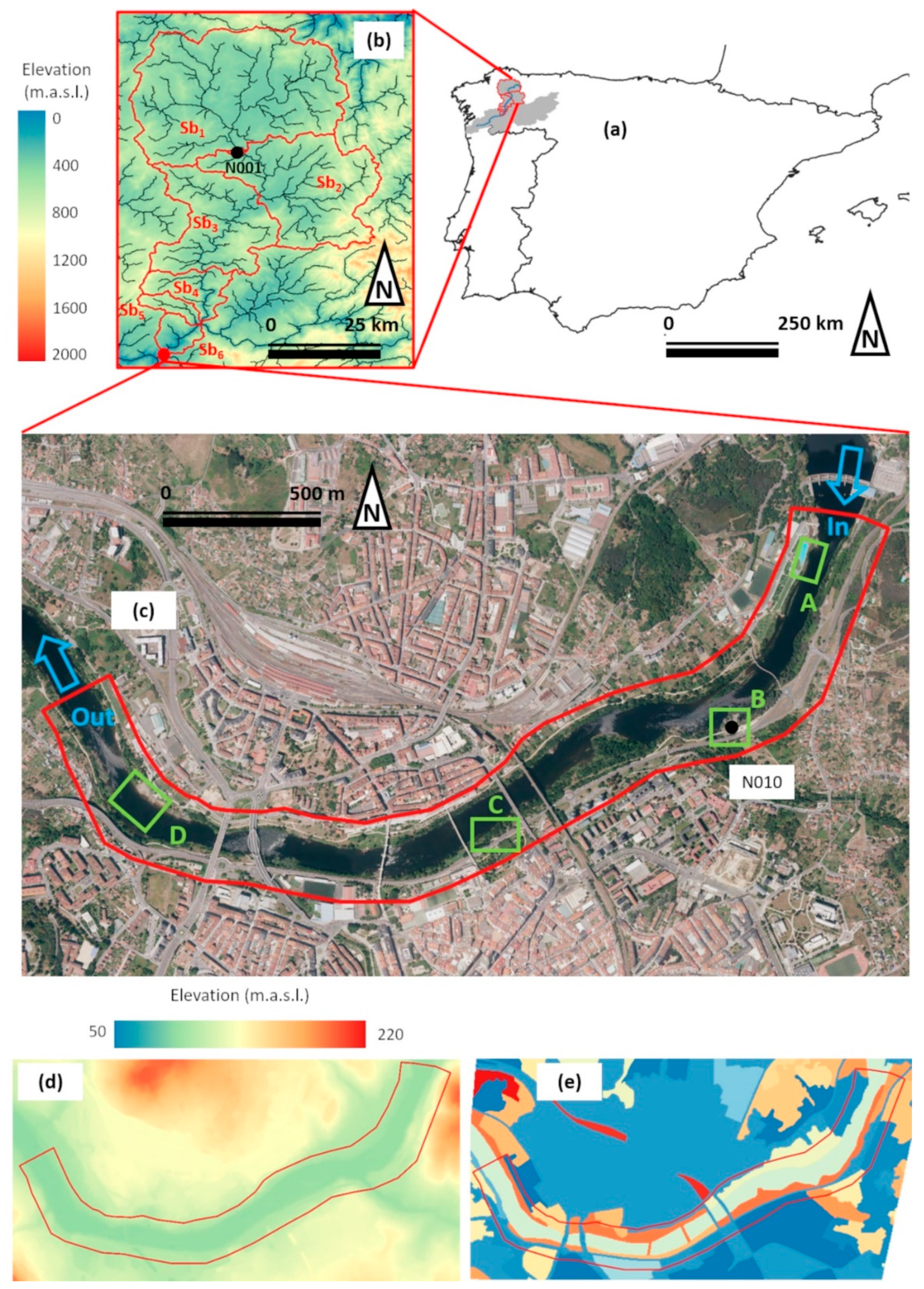
2.1. Study Area

Figure 1 shows the study area analyzed in this work. This area is located in the NW Iberian Peninsula occupying a total extent of around 5000 km2, with an elevation ranging from 90 m.a.s.l. to 1200 m.a.s.l. (Figure 1a,b). It corresponds to the upper reach of the shared Portuguese–Spanish Miño River catchment. The Miño River presents a pluvial regime, with maximum river flows during the winter months and minimum flows during the summer [38]. This flow pattern is regulated by the precipitation characteristics of the area under scope, characterized by a seasonal evolution of Azores high and Iceland low, which provokes the occurrence of most of rainy events during the winter months [39]. Attending to its topographic features, the area under consideration was divided in six sub-basins for the hydrological procedure (Figure 1b). The outlet of the catchment is located at Ourense City (Figure 1c–e), which suppose a critical area affected by recurrent floods under extreme conditions. Attending to these reasons, Ourense is considered to be the test area to analyze the accuracy of the hydraulic model to reproduce flood events. The area delimited by the red line in Figure 1c corresponds to the domain of the hydraulic model. The input and output of the domain are also shown in Figure 1c. The section of the river is 3 km long and the total area is about 1 km2. More than 50 land uses were defined attending to the characteristics of the terrain (Figure 1e).

2.2. Description of the Early Warning System

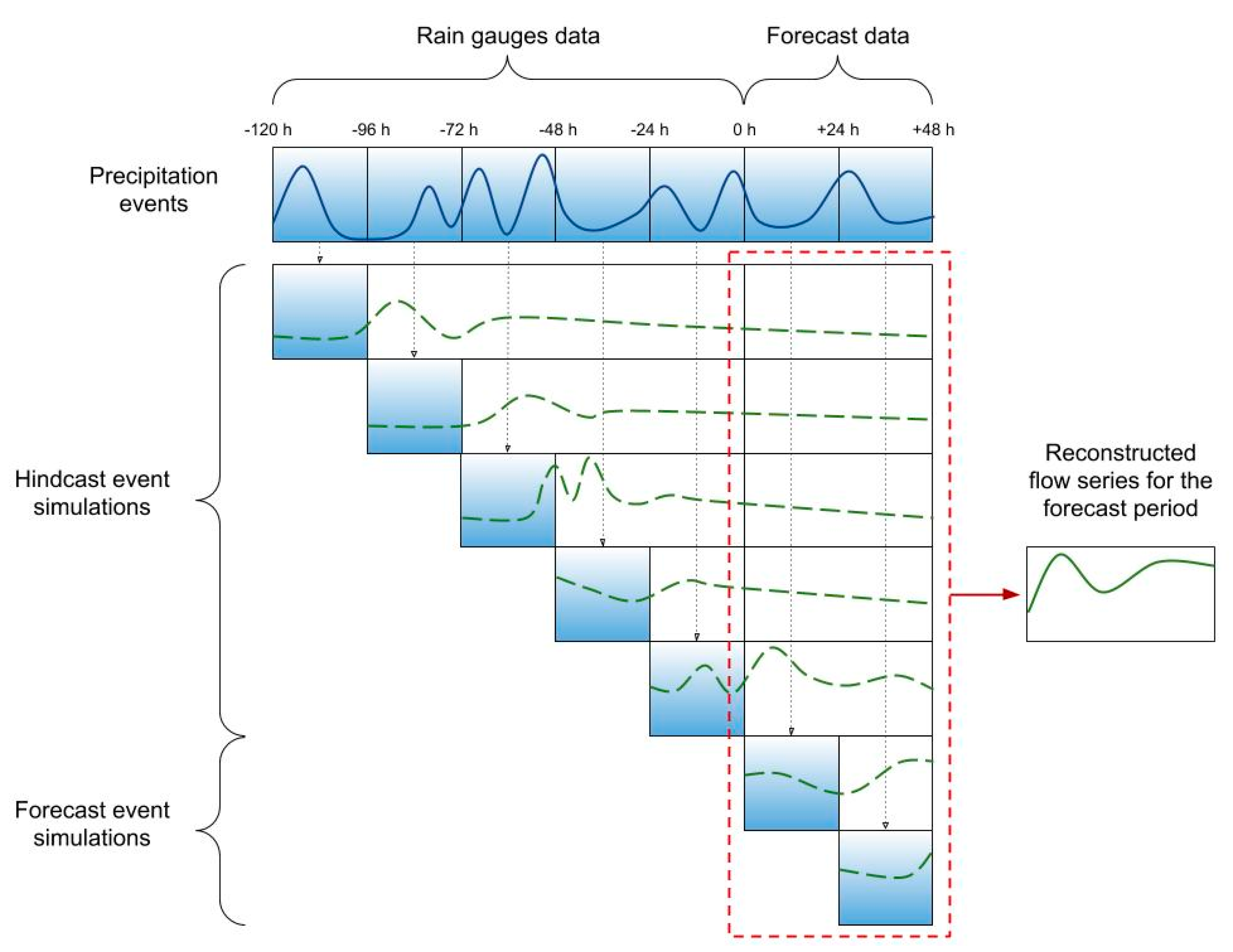
2.2.1. Hydrological Model: HEC-HMS

The semi-distributed model HEC-HMS [40,41] was used to process the main hydrological features of the area under scope. This modelling system, which is one of the most used for hydrological procedures, offers accurate results in locations close to the area under scope [8,31,33]. The designed methodology only requires the input of a few variables to resolve the hydrologic processes—curve number (CN), lag time (Tl), baseflow linear reservoir (BLR), and the routing coefficients along the river channel, as described below.
Rainfall infiltration is determined using the SCS-CN [42,43]. This procedure only requires the knowledge of the CN parameter. The standard CN (intermediate or average conditions) for each sub-basin under scope was firstly calculated following [44,45]:
CN = 25 , 400 S + 254
where S is the potential maximum watershed site storage after runoff begins that is computed using:
S = 5 ( P + 2 Q 4 Q 2 + 5 P Q )
where Q is the runoff depth and P is the rainfall depth, both obtained from SIMPA (stands for integrated precipitation-contribution modelling system) model [46]. Equation (2) is also dependent of initial abstraction, which was simplified as 0.2 · S following Stewart et al. [45], resulting in the equation presented above.
The theoretical CN value obtained at Lugo was calibrated using river flow data provided by the Confederacion Hidrografica del Miño-Sil (CHMS, https://www.chminosil.es). The Lugo location was selected for calibration purposes because the Miño River exists there under natural condition and is not affected by river structures like dams. This procedure was carried out in order to completely adjust the CNs characterizing the area under study. The Nelder–Mead algorithm [47] was used to obtain the optimum value with the Nash–Sutcliffe efficiency index (NSE) as an objective function, which has reported accurate results in surrounding areas [8]. The results obtained show a close relation between the theoretical CN value obtained from Equation (1) and the calibrated value (81 and 84, respectively), which suppose differences of less than 5%. The correction in CN value detected in calibration process was extrapolated to the rest of the sub-basins. First, theoretical values were calculated by means of Equation (1), and then, the correction (in percentage) was applied. In all cases, obtained CNs were rounded to the upper value (Table 1). CN values are similar to the ones obtained in other studies developed in close areas [31].
In addition, it is a well-known fact that this standard CN should be modified attending to the different moisture content of the soil [31,48,49]. This means that the antecedent moisture content (AMC) plays a key role in the rain-runoff processes. The criterion to determine the different conditions is based on [50], which defines three possible CN classes (dry, average, and moist), whose inter-connections are specified in the equations defined in [50].
CN dry = 4.2 × CN average 10 0.058 × CN average
CN moist = 23 × CN average 10 + 0.13 × CN average
The thresholds delimiting the corresponding CN class are also based on the SCS criterion [50], establishing two different annual seasons (non-humid and humid) and a dependence of the cumulative rainfall occurred in the antecedent days. The SCS approach only takes into account the antecedent five days for AMC calculations, however, some studies reveal that the rainfall of a larger number of antecedent days has also an important impact [51,52]. This was also tested in locations close to the area under scope, where [31] detected the important role of the previous 30 days in the moisture content. Slightly better results were obtained in the study area when the AMC of the previous 30 days was considered during the non-humid season and the AMC of the previous 5 days during the humid season (Table 2). In the present work, the non-humid season was calculated to last from April to November and the humid season from December to March. However, some false peaks of river discharge can be obtained in December under the first intense precipitations. To correct this issue, the transition from the non-humid to the humid season starts only when the 30-day AMC surpasses 216 mm (that corresponds with the dry conditions threshold for the non-humid season). Taking into account the considerations commented above, it can be concluded that the conditions that better represent the AMC of the area under scope are those described in Table 2. The obtained thresholds are in accordance with Cea and Fraga [31].
The SCS unit hydrograph was selected to model the transformation of rainfall excess into surface runoff [43,50]. This approach only requires the input of the Lag Time and has shown accurate results for nearby areas [8,33]. First, time of concentration was calculated following the equation proposed by spanish development ministry [53], which provides a good approximation for Spanish basins,
T c = 0.3 × L c 0.76 × J c 0.19
where Tc is the time of concentration in hours, Lc is the length of the longest flow path in kilometers, and Jc is the slope of the longest flow path in m/m.
Then, Lag Time was estimated by means of the approximation proposed by the SCS,
T l = 0.6 × T c
Tl was calibrated at Lugo station following the procedure explained above, obtaining larger values than the theoretical ones for our case of study. After the calibration process, the Tl equation which best represent the area under scope was
T l = 0.37 × L c 0.76 × J c 0.19
This equation was used for all the sub-basins of the study. Lag time values were rounded at hourly scale according to the available time data resolution (Table 1).
Baseflow dynamics was also calibrated at the Lugo station. For that, periods of diminishing flow after precipitation events were evaluated in order to know the constants associated to baseflow routing. These periods were selected several days after the precipitation to ensure that most of the river flow is due to baseflow dynamics. According to previous studies analyzing nearby areas [8], the scheme, which better represents the baseflow dynamics of the area under study, was a linear reservoir with two layers, one of them with a faster response (180 h) than the other (600 h). The results obtained were used for the rest of the sub-basins. Also, it was observed that the baseflow response during the non-humid season was significantly attenuated compared with the humid season. This fact caused false peak values associated to precipitation events during dry season. To overcome this issue, a number between one and three sequential reservoirs was used depending on the average river flow in the previous 30 days. This approach achieves an attenuation in the baseflow response in concordance with the observed river flow.
Regarding the channel routing, the Muskingum–Cunge method [54] was selected, which has provided accurate results in previous studies in close areas [33]. The variables required (river length, slope, width, etc.) were determined according to data obtained from digital terrain models.
Finally, it is important to take into account that the most important tributary of Miño River, the Sil River, is not simulated. This simulation of Sil River flow is not straightforward since the river is highly regulated by a network of connections among dams. However, the Sil River debouches into the Miño River upstream from the city of Ourense, which makes it mandatory to forecast its contribution at that location. To overcome this limitation, the river flow predicted by the hydrological system in Ourense is reconstructed. For that, the system analyzes the relation between simulated river flow (which considers only Miño catchment) and the real flow observed at that location (which also includes the contributions of Sil River) during the period preceding the day under study (24 h and 5 h for the non-humid and humid seasons, respectively). A scale factor between the observed and forecasted flow at Ourense is obtained for the previous day. Then, this factor is applied to the hydrological forecast for the day of interest to take into account the influence of Sil river at this location.

2.2.2. Hydraulic Model: Iber+

Iber [36] is a numerical tool that solves the 2D depth-averaged shallow water equations using the finite volume method. Iber+ [35] is a new implementation of the model in C++ and CUDA [55] to improve the efficiency of the simulations. The new code is able to achieve a two-order of magnitude speed-up while attaining the same precision by using graphical processing unit (GPU) computing high performance computing (HPC) techniques. These optimizations bring the possibility to employ the model in applications with large spatio-temporal domains [56] or time constrained applications [8,33]. The software package is freely available and can be downloaded from its official website (https://iberaula.es). It also includes a graphical user interface (GUI) with preprocessing and post-processing tools.
In the present study, Iber+ was applied to analyze flood events in the test area of the city of Ourense. Figure 1c shows the numerical domain at Ourense, where more than 50 land uses were defined to model the characteristics of the terrain (Figure 1e). Manning’s coefficients were computed accordingly to Gonzalez-Cao et al. [57]. The inlet condition was defined by means of the input hydrograph (critical–subcritical), and the outlet condition was defined using a supercritical–critical outflow. Turbulence was not taken into account as suggested by [58] and in accordance with similar works [59,60,61]. The digital elevation model (DEM) that describes the topography of the area of study has a resolution of 5 m. The DEM data files were obtained from the Instituto Geográfico Nacional website (https://www.ign.es/web/ign/portal). The computational domain was discretized using a mesh with 91,216 unstructured triangular elements, with an average area of 5 m2.

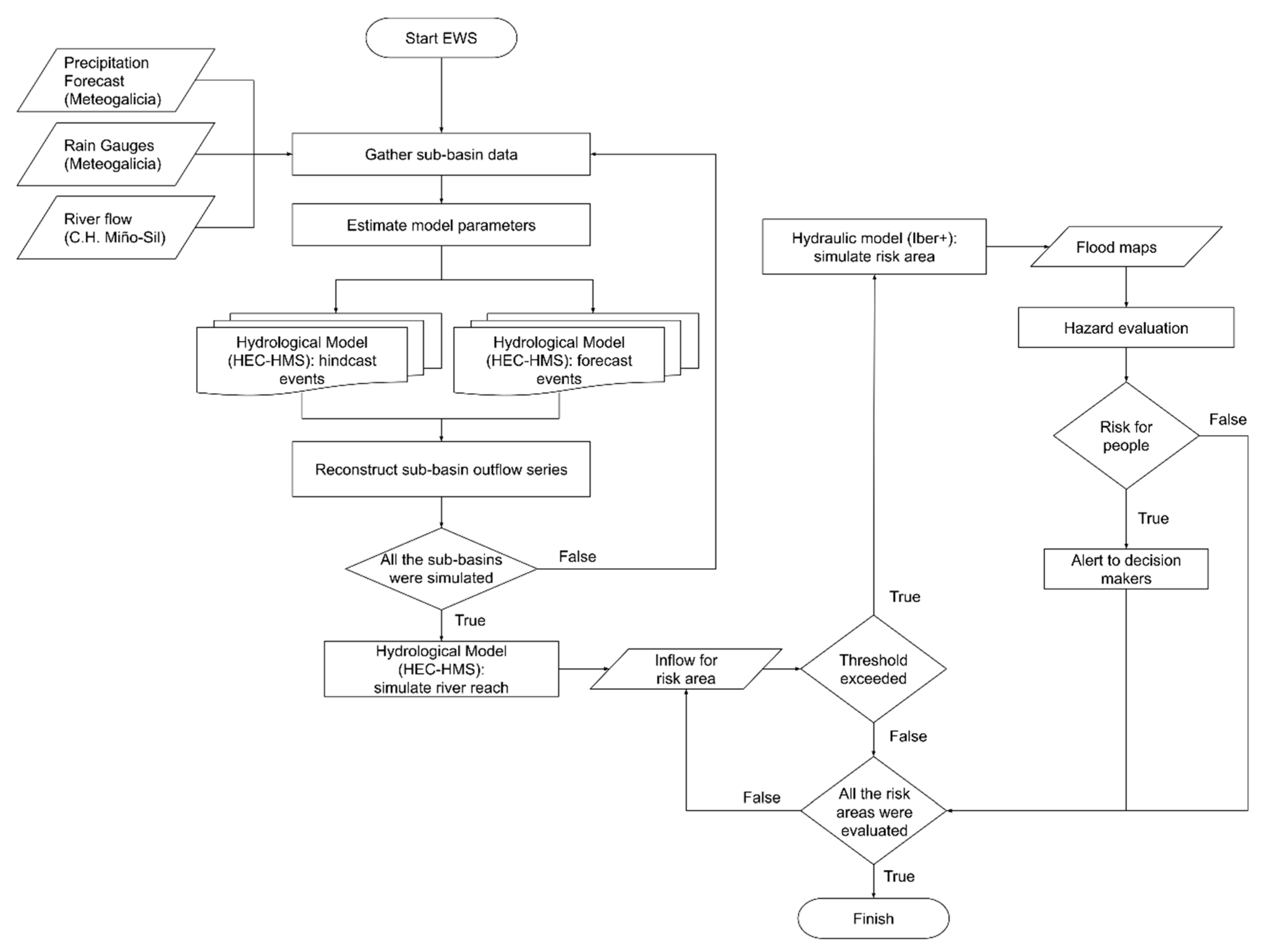
2.2.3. Automatic Early Warning System

The early warning system is governed by a set of Python scripts. Basically, the system is triggered automatically once the precipitation forecasts are published by the local meteorological agency MeteoGalicia (https://www.meteogalicia.gal). MeteoGalicia provides precipitation information with a 72 h forecast window under a temporal and spatial resolution of 1 h and 4 km, respectively, providing an adequately representation of rainy situations for the area under scope [33]. Then, the hydrological simulation is run with the HEC-HMS model, followed by the hydraulic simulations of Iber+ for each area of interest. The computational step and the results of HEC-HMS are on an hourly scale according to the precipitation data. The Iber+ model results are also on hourly scale, while the computational step is adaptive, using a Courant–Friedrichs–Lewy condition [62] value of 0.45. A 24-h forecast horizon is considered. If any hazard is detected, an alert is issued to the corresponding decision makers. The general architecture of the system is shown in Figure 2.
The data necessary to perform the simulations is automatically retrieved by the system. This is the precipitation forecast and rain gauge data for the basins analyzed (from MeteoGalicia) and the current river flow (from CHMS) to determine the initial baseflow of the reach. The separation of the baseflow from the total flow is performed with the Eckhardt method [63], which is applied recursively from an instant where all the flow could be considered as baseflow. It is also important to note that the existing dams were not considered in the present work. However, this is a reasonable approach since, under extreme events, dams have low potential of regulation.
The hydrological simulations are performed with HEC-HMS using an SCS-CN runoff model. Although it was meant for single event simulations, the proposed method was designed to overcome its limitations. For this, the simulation of each sub-basin is separated from the simulation of the river reach. Each sub-basin is simulated for several fixed precipitation events of 24 h (See Figure 3). Each simulated event will have an independent curve number based on the precedent conditions as described above. Additionally, if the simulated event is under the CNmoist class, precipitation of the previous 6 h before the event is also analyzed, and if precipitation exceeds a threshold (8 mm), the CN will be increased to 97 in order to not interrupt the rain-runoff process. The number of forecasted events depends on the period that will be predicted and will take data from the precipitation forecast. The number of hindcast events depend on the characteristics of the basin, for the case of study we found that events prior to five days before the forecast do not have a significant influence on the flow. In the present analysis, the precipitation corresponding to the previous days was estimated from rain gauges, although the system can also run with forecasted precipitation. The second approach is especially useful for poorly sampled areas or in case of malfunction in the rain gauges. The simulations run with precipitation data of a single event (24 h), but the simulation period finishes at the end of the prediction period. Then, the outflow series of the sub-basin is reconstructed with data from each simulation. Starting from the flow series of the forecast simulations, we sum the run-off coming from the previous events and the increments in the baseflow. The resulting flow series represent the flow caused by the forecast events and also the previous ones. The outflow of each sub-basin is then used as input data for the simulation of the river reach. Although this method makes the simulation process more complex, the number of parameters needed is the same as for the regular SCS-CN method, making it especially suitable for those cases were the data needed to parametrize other methods is not available. The proposed method can be applied to simulate longer periods of time than SCS-CN without losing infiltration capacity and adjusting the best CN for each event of that period.
After the hydrological simulation, the hydraulic simulations with Iber+ are triggered for each zone of interest. Simulations can be launched on every EWS execution or only when a certain safety threshold is exceeded in the input flow. This second approach can be especially suitable when the computation resources are limited. Each of the simulations performed with Iber+ are executed in a GPU Nvidia RTX 2080ti and require a computational time in the order of 3–5 min for each 24 h of simulated time for meshes of the order of 70–200 k elements. If the modelled reach contains a high number of zones that require hydraulic simulations, these could be launched in parallel in different GPUs to maintain execution times in reasonable values. These simulations produce water depth and hazard maps for maximum values and hourly values. When some hazard is detected in the hydraulic simulations, an alert is issued to the corresponding decision makers.

2.3. Statistical Parameters to Analyze the Performance of the EWS

Some of the most used statistical parameters to evaluate the performance of this type of procedure were considered to analyze the accuracy of the EWS. In this sense, Spearman coefficient of correlation (r), the ratio of the root mean square error to the standard deviation of the observed data (RSR), Nash–Sutcliffe efficiency coefficient (NSE), percent bias (PBIAS), and Taylor diagrams (in terms of the normalized standard deviation (σn), normalized centered root-mean-square difference (En) and correlation (R)) [64], were evaluated following the equations presented below.
RSR = i = 1 N ( Q i o b s Q i f o r ) 2 i = 1 N ( Q i o b s Q o b s ¯ ) 2
NSE = 1 i = 1 N ( Q i o b s Q i f o r ) 2 i = 1 N ( Q i o b s Q o b s ¯ ) 2
PBIAS = i = 1 N ( Q i o b s Q i f o r ) i = 1 N ( Q i o b s ) × 100
σ n = i = 1 N ( Q i f o r Q f o r ¯ ) 2 N σ o b s
E n = i = 1 N [ ( Q i f o r Q o b s ¯ ) ( Q i o b s Q o b s ¯ ) ] 2 N σ o b s
R = i = 1 N [ ( Q i f o r Q f o r ¯ ) ( Q i o b s Q o b s ¯ ) ] N   σ f o r   σ o b s
where Qobs is the observed value, Qfor is the forecasted value, N is the total number of observed values, barred variables refer to mean values, the subscript n refers to the normalized parameter, subscript i refers to the different samples, and σ is the standard deviation.

3. Results and Discussion

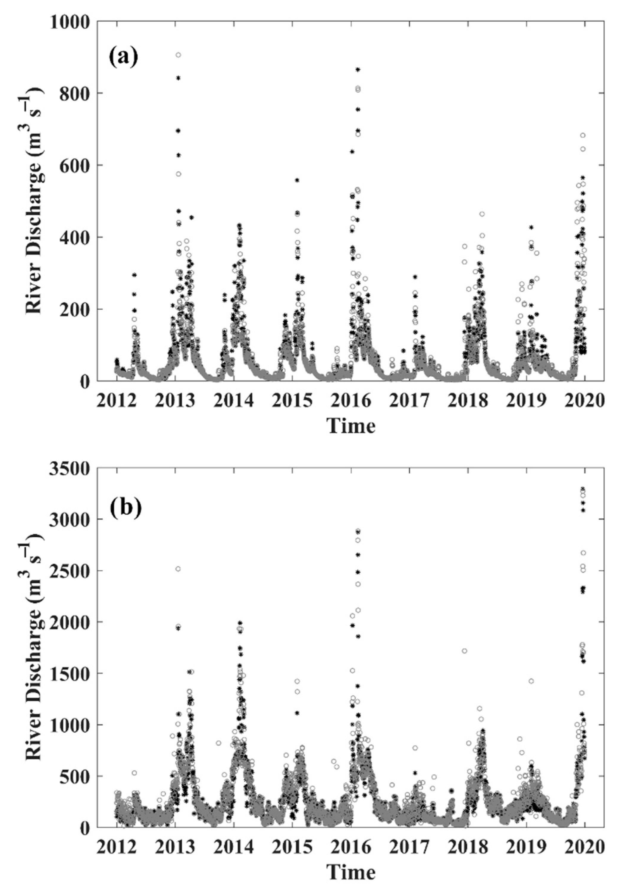
3.1. Hydrologic Module Validation

The accuracy of the hydrological module of the proposed EWS was evaluated by means of statistical analysis respect to measured river discharge data at Lugo and Ourense stations.
When considering the flow data for the studied period in a daily scale, the results show that the model is able to predict with a good degree of accuracy the annual cycle of river flow. The model also shows a clear contrast between dry and humid seasons and is able to reflect the high flow conditions (Figure 4). This is corroborated when the statistical parameters are analyzed (Table 3). It is considered a “very good” performance of a hydrological model when the NSE value surpasses 0.7 and the absolute value of PBIAS is lower than 25% [65,66,67], these parameters are widely fulfilled in the present case (NSE > 0.85 and |PBIAS| < 10%) (Table 3). Moreover, the high correlation detected (r > 0.90) along with the low RSR values obtained (RSR < 0.40) also indicate a good performance according to Moriasi et al. [65], showing the robustness of the methodology developed.
In addition, the most important flood events, whose prediction supposes the critical and main objective from the point of view of EWS, were also evaluated at hourly scale. In particular, those events where river flow surpassed the 99th percentile for the period under study, were taken into account. Analyzing the statistical parameters, model results show an accurate prediction of the real river flow under extreme conditions (Table 4). NSE (>0.7) and |PBIAS| (<7%) values indicate “very good” accuracy of the model developed, which is corroborated by the high correlation values (r > 0.85) along with the low RSR values obtained (<0.55) (Table 4). The statistical analysis shows the high accuracy of the proposed EWS to detect and predict the most important flood events. This is also corroborated in Figure 5, which shows the comparison between the model forecast and the measured river flow under the most dangerous events occurring during the study period at Lugo and Ourense stations. Despite small deviations in the shape of the series, both events were well predicted both in terms of time and magnitude.
It is important to remark that PBIAS values obtained in Table 3 and Table 4 indicate a slight overestimation of predicted river flows. However, this type of systems should be conservative, because the consequences of under-estimate flood events may cause severe damage [8]. In addition, statistical values show a better performance at the Lugo than at the Ourense location, both in the total series length and in the particular case of the extreme events. This is partly due to the fact that the Miño River at Lugo is under natural flow conditions, whereas several dams control the flow at Ourense, along with the fact that the Sil Tiver influence at Ourense is not directly simulated but extrapolated from Miño data as described above.
When the obtained results are compared with other systems developed in nearby areas, the hydrological module shows its potential as river flow predictor. Fraga et al. [8] also use the HEC-HMS hydrological model, but under a continuous simulation mode in nearby areas. This model is divided into the following two stages: hindcast and forecast. During the first stage (hindcast), the hydrological model assimilates several measured data of 30 previous days in order to reproduce the initial soil moisture content at the beginning of the second stage (forecast) by tuning the parameters associated to the infiltration of the terrain. In the forecast stage the river hydrograph is computed. Although it is important to note Fraga et al. [8] focused on small Galician catchments, where hydrological forecast is more sensitive to precipitation distribution, improved values of r and PBIAS are obtained in the present work, which reinforces the robustness of the methodology proposed. Vieira et al. [68] presented a flood forecast system developed for two sub-basins of Ave River catchment (northern Portugal) based on the Delft FEWS platform. In this case the meteorological data are obtained from an ensemble of precipitation predictions. The implementation of the hydrologic and hydraulic models was carried out using SOBEK software. The calibration of the model parameters was developed starting from values obtained in the literature and soil characteristics and using the RRL toolkit. Statistical values are only shown for historical validation period and daily time scale. The EWS developed in the present work achieves statistical values remarking a higher accuracy even considering forecast simulations. A grid-based distributed rainfall-runoff model (GFWS) was implemented in the Guadalhorce basin (southern Spain) [69], which is a poorly gauged basin, in contrast to the basin analyzed in our work. The parameters of the model obtained for a small area of the catchment are transferred to the entire catchment of the Guadalhorce River. In this work, flood warnings obtained with the GFWS model were compared with those obtained with the low resolution EFAS model. Higher values of Nash efficiency for forecasted flood events were also obtained in the present work, showing the good performance of MIDAS.
Therefore, it can be concluded that the hydrological module of the system presented in this work is able to forecast with high accuracy both the annual cycle (continuous) river flow and the extreme flood events. The little discrepancies observed between forecasted numerical and measured river flow can be due to the limitations of these systems—mainly, the simplification of the modelled system and the uncertainty of the forecast precipitation data. In this sense, the hydrological model supposes an approximate representation of the reality; therefore, some discrepancies will be expected. Moreover, although precipitation forecasts provided by MeteoGalicia predict rainy events accurately as shown in González-Cao et al. [33], the precipitation forecast is, by itself, a source of uncertainty, especially under situations of extreme rainfall events [33]. Additionally, rain representation provided by rain gauges can suppose another source of uncertainty. Rain gauges can provide a biased view of the area under scope since they do not cover the subareas of the basins uniformly. Even with these limitations, the system proposed provides a great accuracy to predict river flow, especially under extreme flood events, which impacts the performance MIDAS.

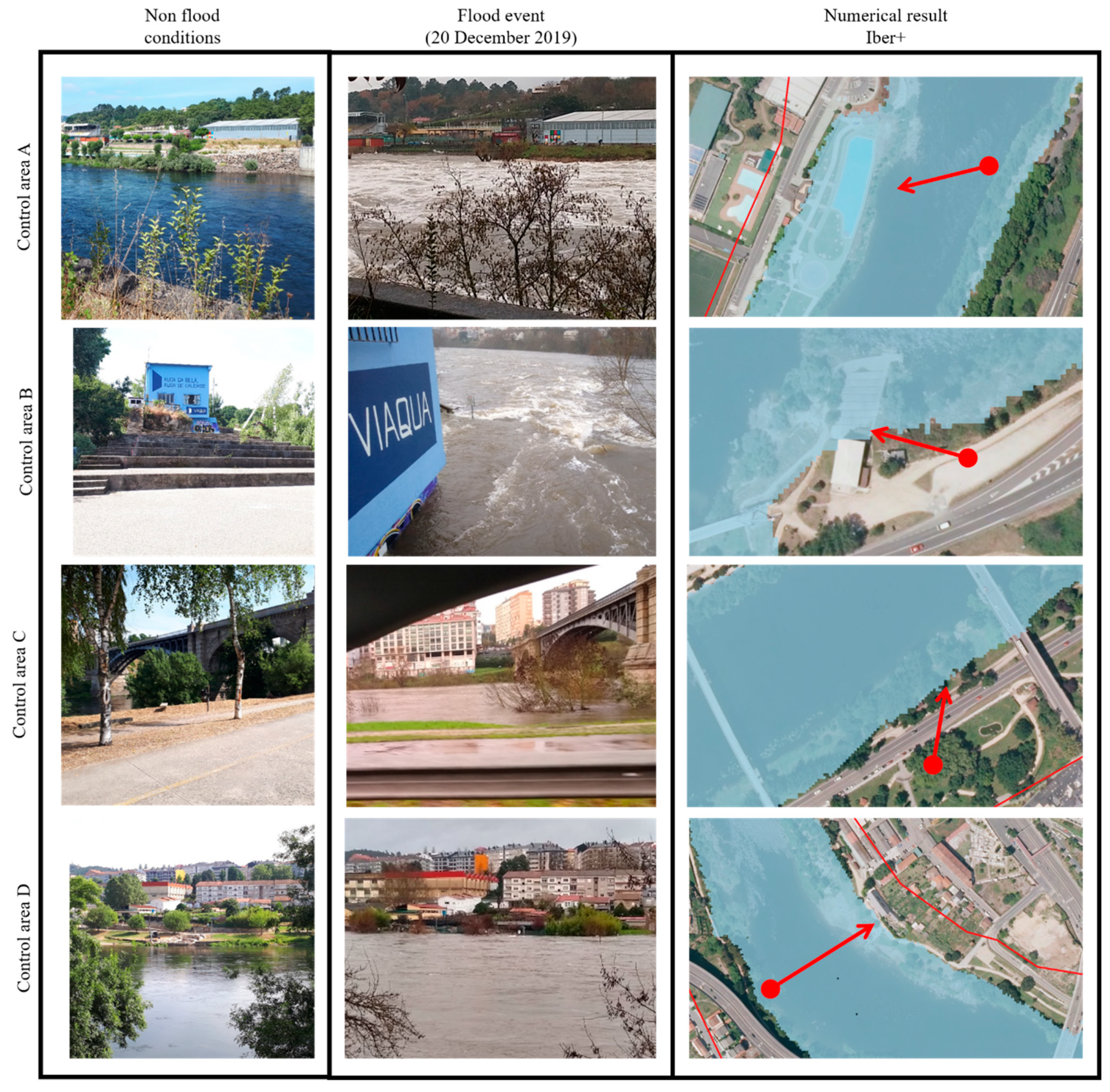
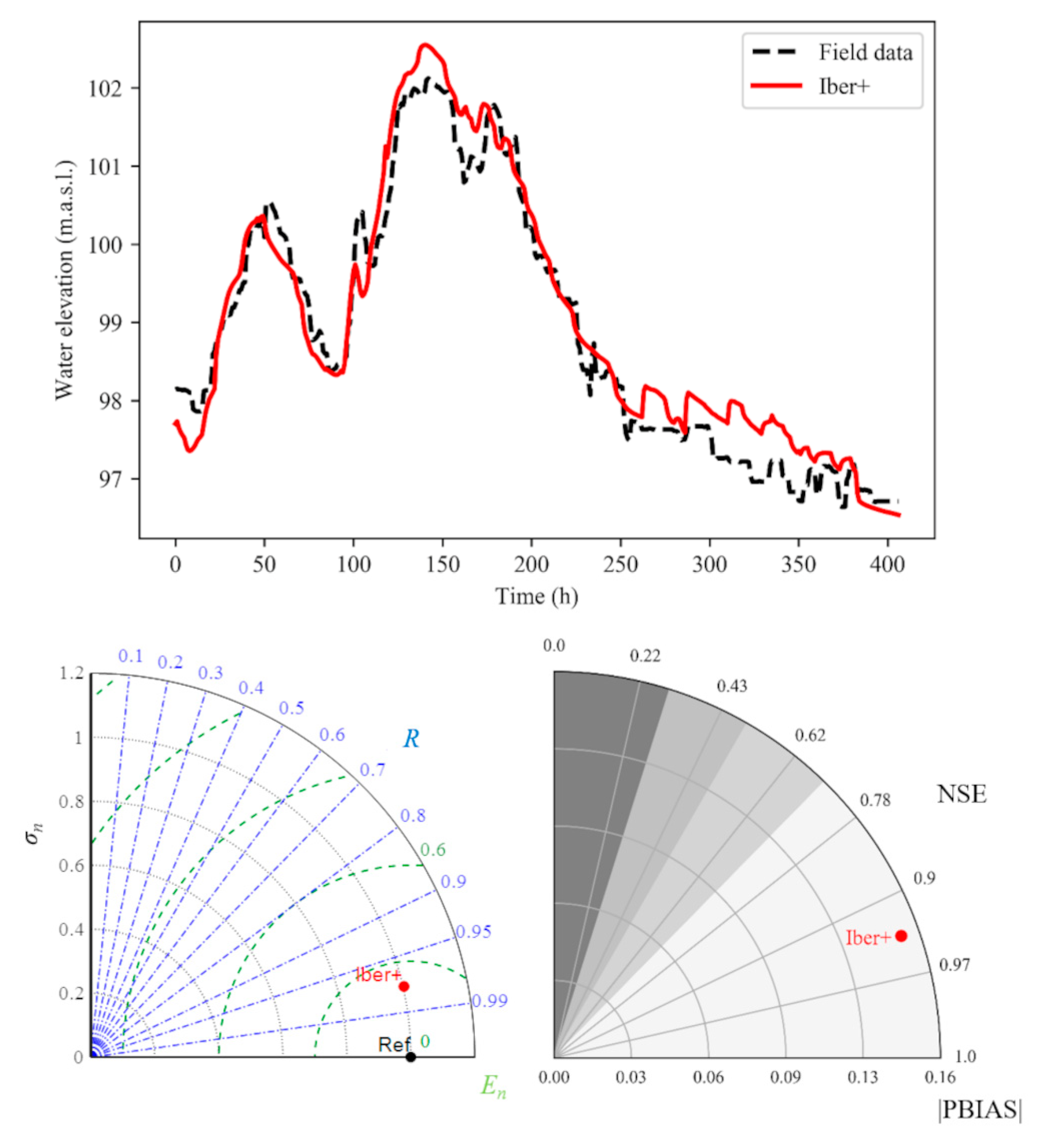
3.2. Hydraulic Module Validation

Once the predicted water flow was shown to reproduce the actual flows with a high accuracy, the performance of the hydraulic model was also analyzed. For that, the extent and the water elevation of the flood event registered on December 2019 (from 15 to 31) were computed using Iber+ [17]. On the one hand, four control areas were defined at study area (green rectangles A, B, C, and D in Figure 1c) to analyze the accuracy of the numerical results of the flood extension. The control area A corresponds with a public sport facility (swimming pool) and its recreational zone, the control area B is located near the gauge station N010 of the CHMS, control area C corresponds with a public path near a national road, and control area D corresponds to a public thermal baths area. All these control areas are located near the riverbank and are usually frequented by pedestrians, therefore being of special interest to issue an alert. On the other hand, the water elevation registered at the gauge station located in control area B was used to compute the accuracy of the numerical water elevation obtained with Iber+ by means of Taylor and NSE vs. |PBIAS| diagrams.
Figure 6 shows the extent of the flood obtained in the numerical simulations along with photographs taken at the control areas during the flood event within the interval 16:00–16:30 UTC (for all times throughout the paper) on 20 December 2019. Images corresponding to non-flood conditions are also depicted, corresponding to a flow within the interval 262–267 m3 s−1 (data obtained from CHMS). The comparison between photographs taken during the flood and non-flood conditions reveals the magnitude of the flood event. Visually, the numerical results are quite similar to the field data. The image of the flood event at the control area A shows that the swimming pool is fully covered by the flood. The numerical result shows the same situation: the water covers the facility and reaches the wall near the road. The image at the control area B shows that the flood reaches the building of the gauge station. The results obtained with Iber+ shows an equivalent situation. Also, the numerical results show that the flood almost reaches the road. The image corresponding to the control area C shows the same situation as the numerical results: the flood extension covers the public path and almost reaches the road. Finally, the thermal baths are fully covered by the flood, and the water almost reaches the path behind them, as can be observed in the photograph at the control area D. The numerical results are equivalent to the image of real event.
The results of the time series of water elevation registered from 15 December 2019 to 31 December 2019 at gauge station N010 are depicted in Figure 7. This figure shows the time series of the water elevation registered at the gauge station (control area B, Figure 1) and the numerical time series obtained with Iber+. Visually, numerical results are similar to field data, which shows the capability of the model to forecast water elevation accordingly with the river discharge forecast (Figure 5b). The Taylor and the NSE vs. |PBIAS| diagrams are also depicted. Taylor diagram shows that the values of σn, En, and R are 1.00, 0.22, and 0.97, respectively. The values of NSE and |PBIAS| depicted in the NSE vs. PBIAS diagram are 0.94 and 0.15%. The circle marker in this diagram denotes a negative value of PBIAS. Shaded areas of the diagram refer to the accuracy level of the results according to the criterion of Yilmaz and Onoz [67]. In this case, the results are in the range corresponding to “very good” improving to some extent the results obtained by Fraga et al. [8] in nearby small catchments. In summary, both diagrams show high agreement between numerical and registered values of water elevation. This indicates that the system can reproduce this kind of events with high accuracy and can be used to issue an alert.

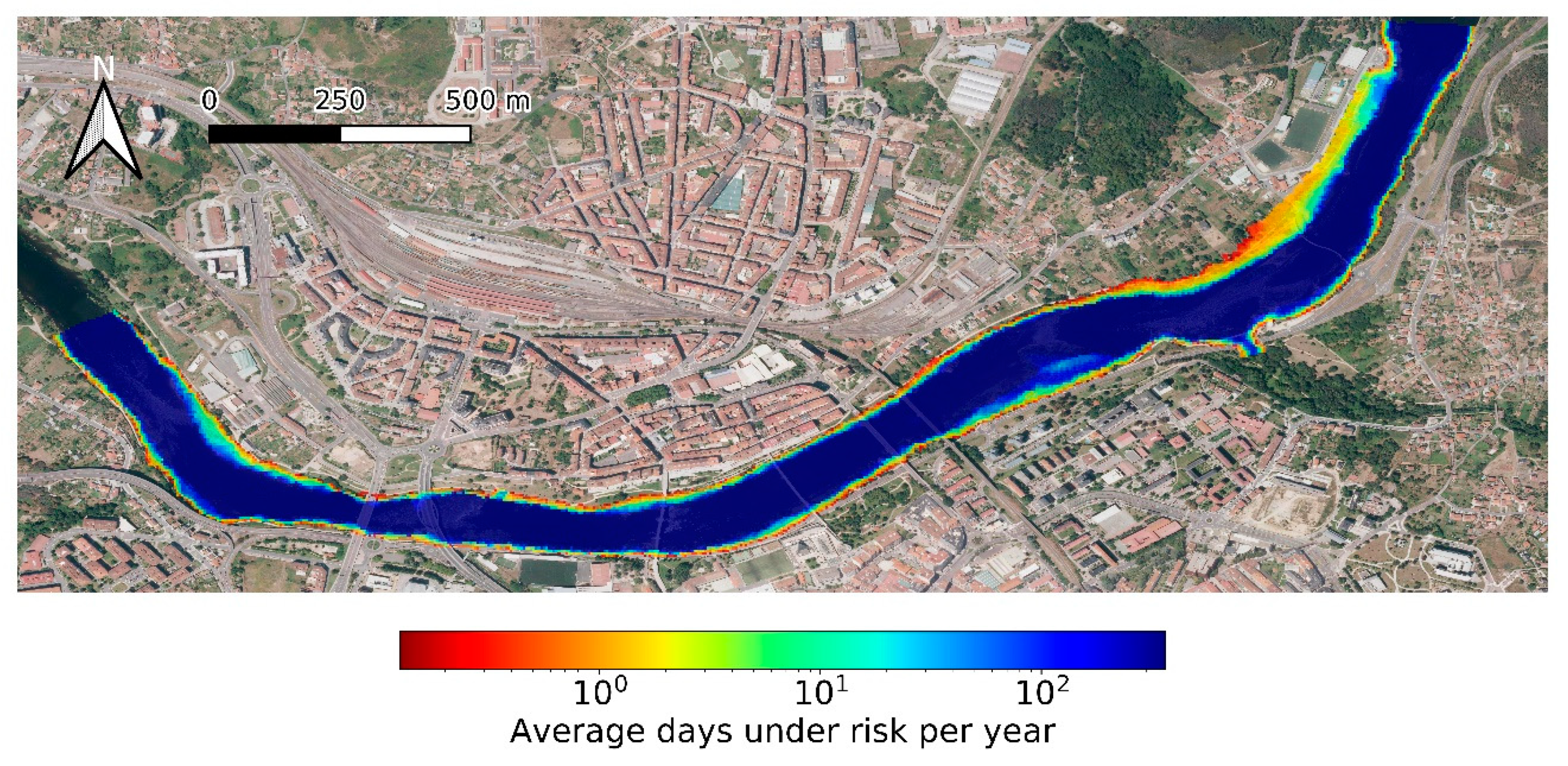
3.3. Analysis and Predictability of River Flood Risk Situations

The validation of the hydrologic and hydraulic modules has shown a good forecast of river flow under flood events as well as a good representation of the areas affected by these flood events. The final step is to focus the system on critical areas from the point of view of critical infrastructures damage. The ultimate goal is that the system can report dangerous situations well in advance so that decision makers can take appropriate mitigation measures. In this sense, the hazard in the city of Ourense is analyzed. The criterion employed to define a hazard area was the presented by Cox et al. [70]. First of all, after am in-depth study of the hazardous areas affected by different water flows, the alert status was divided in four levels (see Table 5 for specific thresholds). The first of them, pre-activation, defines the average conditions of the river reach. In the second level, activation, some risk can occur in areas accessible to but not frequented by pedestrians. The third state is pre-alert where hazard can occur in areas frequented by pedestrians. The last one is the alert state where the flood causes hazard in areas frequented by pedestrians and severe damage to infrastructures.
Once the thresholds that define the different risk situations were evaluated, an analysis of the observed and predicted flow was carried out in order to assess the EWS’s ability to accurately issue an alert. In this sense, 17 alerts should have been issued based on the flow observed during the eight years of the simulated period (Table 6). The EWS accurately predicted 13 of them, 4 were missed and 5 were false positives. This means that the proposed system is able to predict the 76% of the alerts and 28% of the alerts issued are false positives, which shows a good performance of the designed system in terms of predictability of risk situations.
The system is able to issue an alert based on the hydrological forecast and also to provide detailed water depth, water velocity, and hazard maps in terms of hydraulic model simulations. Both the maximum values and hourly evolution of these parameters are obtained for the forecasted period. Figure 8 shows the average number of days under hazard conditions per year. It can be observed that many zones frequented during outdoor activities can be affected by hazard conditions for more than 10 days per year on average, emphasizing the requirement of an accurate EWS. Figure 9 shows the maximum extension of the hazardous area for each of the warning levels defined in Table 5. This map shows that the differences between two warning levels are minimal in certain areas, illustrating the necessity of accompanying the alert reports with detailed flood maps. This information provides a detailed view of areas affected under the respective flood event. In this way, decision makers can have enough data to evaluate the situation correctly and take more precise and effective measures, diminishing the damage provoking by floods.

4. Conclusions

This paper presents MIDAS, a new flood early warning system based on integrated hydrologic and hydraulic models. The automatic operation of MIDAS is governed by a set of Python scripts. Starting from precipitation forecast, the rainfall-runoff process is simulated with the HEC-HMS model to obtain the predicted river flow, which is used to run Iber+ for each area of interest. An alert is issued when a hazardous situation is detected.
The results show the high capability of the system to accurately forecast river flows and are representative of the flooded areas under extreme events. In fact, MIDAS was able to predict 13 of the 17 alerts that took place over the study period, which is a good performance in terms of predictability of risk situations. This good performance of the system, together with the capability to provide detailed hazard maps, can provide information to decision makers to evaluate flood situations and to take precise and effective measures that mitigate the damage associated with these events.
Finally, it is important to remark that, despite MIDAS being applied to the Miño River, its implementation in other basins is straightforward. This approach is especially valuable for areas with low sampling resources, showing its potential in future applications.

Author Contributions

D.F.-N., O.G.-F., J.G.-C., and M.G.-G. conceived the study; D.F.-N., O.G.-F., and J.G.-C. conducted the research and developed the software; M.G.-G. supervised the research development; D.F.-N., O.G.-F., J.G.-C., C.d.G., J.A.R.-S., C.R.d.P., and M.G.-G. analyzed the results; D.F.-N., O.G.-F., J.G.-C., and M.G.-G. wrote the manuscript; C.d.G., J.A.R.-S., and C.R.d.P supervised the research, provided field data, and revised the manuscript. All authors have read and agreed to the published version of the manuscript.

Funding

This research was partially supported by INTERREG-POCTEP under project RISC_ML (Code: 0034_RISC_ML_6_E) co-funded by the European Regional Development Fund (ERDF) and by Xunta de Galicia under Project ED431C 2017/64-GRC “Programa de Consolidación e Estruturación de Unidades de Investigación Competitivas (Grupos de Referencia Competitiva).” O.G.F. is supported by Xunta de Galicia grant ED481A-2017/314.

Acknowledgments

The aerial pictures used in this work are courtesy of the Spanish Instituto Geográfico Nacional (IGN) and part of the Plan Nacional de Ortofotografía Aérea (PNOA) program.

Conflicts of Interest

The authors declare no conflict of interest. The funders had no role in the design of the study; in the collection, analyses, or interpretation of data; in the writing of the manuscript, or in the decision to publish the results.

References

  1. Berghuijs, W.R.; Aalbers, E.E.; Larsen, J.R.; Trancoso, R.; Woods, R.A. Recent changes in extreme floods across multiple continents. Environ. Res. Lett. 2017, 12, 114035. [Google Scholar] [CrossRef]
  2. Passerotti, G.; Massazza, G.; Pezzoli, A.; Bigi, V.; Zsótér, E.; Rosso, M. Hydrological Model Application in the Sirba River: Early Warning System and GloFAS Improvements. Water 2020, 12, 620. [Google Scholar] [CrossRef] [Green Version]
  3. Rosburg, T.T.; Nelson, P.A.; Bledsoe, B.P. Effects of Urbanization on Flow Duration and Stream Flashiness: A Case Study of Puget Sound Streams, Western Washington, USA. JAWRA J. Am. Water Resour. Assoc. 2017, 53, 493–507. [Google Scholar] [CrossRef]
  4. Booth, D.B.; Bledsoe, B.P. Streams and urbanization. In The Water Environment of Cities; Baker, L.A., Ed.; Springer: Boston, MA, USA, 2009; pp. 93–123. ISBN 978-0-387-84891-4. [Google Scholar]
  5. Arnell, N.W.; Gosling, S.N. The impacts of climate change on river flood risk at the global scale. Clim. Chang. 2016, 134, 387–401. [Google Scholar] [CrossRef] [Green Version]
  6. Liu, C.; Guo, L.; Ye, L.; Zhang, S.; Zhao, Y.; Song, T. A review of advances in China’s flash flood early-warning system. Nat. Hazards 2018, 92, 619–634. [Google Scholar] [CrossRef] [Green Version]
  7. Alfieri, L.; Salamon, P.; Pappenberger, F.; Wetterhall, F.; Thielen, J. Operational early warning systems for water-related hazards in Europe. Environ. Sci. Policy 2012, 21, 35–49. [Google Scholar] [CrossRef]
  8. Fraga, I.; Cea, L.; Puertas, J. MERLIN: A flood hazard forecasting system for coastal river reaches. Nat. Hazards 2020, 100, 1171–1193. [Google Scholar] [CrossRef]
  9. Groisman, P.Y.; Knight, R.W.; Easterling, D.R.; Karl, T.R.; Hegerl, G.C.; Razuvaev, V.N. Trends in Intense Precipitation in the Climate Record. J. Clim. 2005, 18, 1326–1350. [Google Scholar] [CrossRef]
  10. Beniston, M. Trends in joint quantiles of temperature and precipitation in Europe since 1901 and projected for 2100. Geophys. Res. Lett. 2009, 36. [Google Scholar] [CrossRef] [Green Version]
  11. Morss, R.E.; Wilhelmi, O.V.; Meehl, G.A.; Dilling, L. Improving Societal Outcomes of Extreme Weather in a Changing Climate: An Integrated Perspective. Annu. Rev. Environ. Resour. 2011, 36, 1–25. [Google Scholar] [CrossRef] [Green Version]
  12. Wallemacq, P.; House, R.; Below, R.; McLean, D. Economic Losses, Poverty & Disasters: 1998–2017; Centre for Research on the Epidemiology of Disasters (CRED); United Nations Office for Disaster Risk Reduction (UNISDR): Brussels, Belgium, 2018. [Google Scholar]
  13. Han, L.; Xu, Y.; Pan, G.; Deng, X.; Hu, C.; Xu, H.; Shi, H. Changing properties of precipitation extremes in the urban areas, Yangtze River Delta, China, during 1957–2013. Nat. Hazards 2015, 79, 437–454. [Google Scholar] [CrossRef]
  14. Hallegatte, S. A Cost Effective Solution to Reduce Disaster Losses in Developing Countries: Hydro-Meteorological Services, Early Warning, and Evacuation; The World Bank: Washington, DC, USA, 2012. [Google Scholar]
  15. Cools, J.; Innocenti, D.; O’Brien, S. Lessons from flood early warning systems. Environ. Sci. Policy 2016, 58, 117–122. [Google Scholar] [CrossRef]
  16. Borga, M.; Anagnostou, E.N.; Blöschl, G.; Creutin, J.-D. Flash flood forecasting, warning and risk management: The HYDRATE project. Environ. Sci. Policy 2011, 14, 834–844. [Google Scholar] [CrossRef]
  17. Thielen, J.; Bartholmes, J.; Ramos, M.-H.; de Roo, A. The European Flood Alert System—Part 1: Concept and development. Hydrol. Earth Syst. Sci. 2009, 13, 125–140. [Google Scholar] [CrossRef] [Green Version]
  18. Pappenberger, F.; Thielen, J.; Medico, M.D. The impact of weather forecast improvements on large scale hydrology: Analysing a decade of forecasts of the European Flood Alert System. Hydrol. Process. 2011, 25, 1091–1113. [Google Scholar] [CrossRef]
  19. Alfieri, L.; Pappenberger, F.; Wetterhall, F.; Haiden, T.; Richardson, D.; Salamon, P. Evaluation of ensemble streamflow predictions in Europe. J. Hydrol. 2014, 517, 913–922. [Google Scholar] [CrossRef] [Green Version]
  20. Bartholmes, J.C.; Thielen, J.; Ramos, M.H.; Gentilini, S. The european flood alert system EFAS—Part 2: Statistical skill assessment of probabilistic and deterministic operational forecasts. Hydrol. Earth Syst. Sci. 2009, 13, 141–153. [Google Scholar] [CrossRef] [Green Version]
  21. Alfieri, L.; Burek, P.; Dutra, E.; Krzeminski, B.; Muraro, D.; Thielen, J.; Pappenberger, F. GloFAS—global ensemble streamflow forecasting and flood early warning. Hydrol. Earth Syst. Sci. 2013, 17, 1161–1175. [Google Scholar] [CrossRef] [Green Version]
  22. Corral, C.; Berenguer, M.; Sempere-Torres, D.; Poletti, L.; Silvestro, F.; Rebora, N. Comparison of two early warning systems for regional flash flood hazard forecasting. J. Hydrol. 2019, 572, 603–619. [Google Scholar] [CrossRef] [Green Version]
  23. Hirpa, F.A.; Hopson, T.M.; De Groeve, T.; Brakenridge, G.R.; Gebremichael, M.; Restrepo, P.J. Upstream satellite remote sensing for river discharge forecasting: Application to major rivers in South Asia. Remote Sens. Environ. 2013, 131, 140–151. [Google Scholar] [CrossRef]
  24. Cloke, H.L.; Pappenberger, F. Ensemble flood forecasting: A review. J. Hydrol. 2009, 375, 613–626. [Google Scholar] [CrossRef]
  25. De Luca, D.L.; Biondi, D.; Capparelli, G.; Galasso, L.; Versace, P. Mathematical models for early warning systems. IAHS-AISH Publ. 2010, 340, 485–495. [Google Scholar]
  26. Baudoin, M.-A.; Henly-Shepard, S.; Fernando, N.; Sitati, A.; Zommers, Z. Early Warning Systems and Livelihood Resilience: Exploring Opportunities for Community Participation; UNU-EHS Working Paper Series; United Nations University: Tokyo, Japan, 2014. [Google Scholar]
  27. Ritter, J.; Berenguer, M.; Corral, C.; Park, S.; Sempere-Torres, D. ReAFFIRM: Real-time Assessment of Flash Flood Impacts–a Regional high-resolution Method. Environ. Int. 2020, 136, 105375. [Google Scholar] [CrossRef] [PubMed]
  28. Collier, C.G. Flash flood forecasting: What are the limits of predictability? Q. J. R. Meteorol. Soc. 2007, 133, 3–23. [Google Scholar] [CrossRef]
  29. de Gonzalo, C.; Robredo, J.C.; Mintegui, J.Á. Semidistributed hydrologic model for flood risk assessment in the Pejibaye River Basin, Costa Rica. J. Hydrol. Eng. 2012, 17, 1333–1344. [Google Scholar] [CrossRef]
  30. De Silva, M.; Weerakoon, S.B.; Herath, S. Modeling of event and continuous flow hydrographs with HEC–HMS: Case study in the Kelani River Basin, Sri Lanka. J. Hydrol. Eng. 2014, 19, 800–806. [Google Scholar] [CrossRef]
  31. Cea, L.; Fraga, I. Incorporating antecedent moisture conditions and intraevent variability of rainfall on flood frequency analysis in poorly gauged basins. Water Resour. Res. 2018, 54, 8774–8791. [Google Scholar] [CrossRef]
  32. Wang, D. A new probability density function for spatial distribution of soil water storage capacity leads to the SCS curve number method. Hydrol. Earth Syst. Sci. 2018, 22, 6567–6578. [Google Scholar] [CrossRef] [Green Version]
  33. González-Cao, J.; García-Feal, O.; Fernández-Nóvoa, D.; Domínguez-Alonso, J.M.; Gómez-Gesteira, M. Towards an automatic early warning system of flood hazards based on precipitation forecast: The case of the Miño River (NW Spain). Nat. Hazards Earth Syst. Sci. 2019, 19. [Google Scholar] [CrossRef] [Green Version]
  34. Nguyen, P.; Thorstensen, A.; Sorooshian, S.; Hsu, K.; AghaKouchak, A.; Sanders, B.; Koren, V.; Cui, Z.; Smith, M. A high resolution coupled hydrologic–hydraulic model (HiResFlood-UCI) for flash flood modeling. J. Hydrol. 2016, 541, 401–420. [Google Scholar] [CrossRef] [Green Version]
  35. García-Feal, O.; González-Cao, J.; Gómez-Gesteira, M.; Cea, L.; Domínguez, J.M.; Formella, A. An accelerated tool for flood modelling based on Iber. Water 2018, 10, 1459. [Google Scholar] [CrossRef] [Green Version]
  36. Bladé, E.; Cea, L.; Corestein, G.; Escolano, E.; Puertas, J.; Vázquez-Cendón, E.; Dolz, J.; Coll, A. Iber: Herramienta de simulación numérica del flujo en ríos. Revista Internacional de Métodos Numéricos para Cálculo y Diseño en Ingeniería 2014, 30, 1–10. [Google Scholar] [CrossRef] [Green Version]
  37. Lorenzo, M.N.; Alvarez, I. Climate change patterns in precipitation over Spain using CORDEX projections for 2021–2050. Sci. Total Environ. 2020, 138024. [Google Scholar] [CrossRef] [PubMed]
  38. Fernández-Nóvoa, D.; deCastro, M.; Des, M.; Costoya, X.; Mendes, R.; Gómez-Gesteira, M. Characterization of Iberian turbid plumes by means of synoptic patterns obtained through MODIS imagery. J. Sea Res. 2017, 126, 12–25. [Google Scholar] [CrossRef]
  39. deCastro, M.; Lorenzo, N.; Taboada, J.J.; Sarmiento, M.; Alvarez, I.; Gomez-Gesteira, M. Influence of teleconnection patterns on precipitation variability and on river flow regimes in the Miño River basin (NW Iberian Peninsula). Clim. Res. 2006, 32, 63–73. [Google Scholar] [CrossRef] [Green Version]
  40. Feldman, A.D. Hydrologic Modeling System HEC-HMS: Technical Reference Manual; USA Army Corps of Engineers: Washington, DC, USA; Hydrologic Engineering Center: Davis, CA, USA, 2000.
  41. Scharffenberg, B.; Bartles, M.; Brauer, T.; Fleming, M.; Karlovits, G. Hydrologic Modeling System (HEC-HMS). User’s Manual: Version 4.3; USA Army Corps of Engineers: Washington, DC, USA, 2018.
  42. USA Department of Agriculture. Soil Conservation Service (SCS) “Hydrology” National Engineering Handbook; Section 4; USA Department of Agriculture: Washington, DC, USA, 1985.
  43. USA Department of Agriculture. NRCS: Natural Resources Conservation Service National Engineering Handbook; Chapter 16 Hydrographs; USA Department of Agriculture: Washington, DC, USA, 2007.
  44. Soil Conservation Service (SCS). Technical Release 55: Urban Hydrology for Small Watersheds, 2nd ed.; USA Department of Agriculture: Washington, DC, USA, 1986.
  45. Stewart, D.; Canfield, E.; Hawkins, R. Curve number determination methods and uncertainty in hydrologic soil groups from semiarid watershed data. J. Hydrol. Eng. 2012, 17, 1180–1187. [Google Scholar] [CrossRef]
  46. Ministerio para la Transición Ecológica y el Reto Demográfico, Spain Government Modelo SIMPA 2019. Periodo de simulación: 1940/41 a 2017/18. Available online: https://www.miteco.gob.es/es/agua/temas/evaluacion-de-los-recursos-hidricos/evaluacion-recursos-hidricos-regimen-natural/ (accessed on 22 June 2020).
  47. Nelder, J.A.; Mead, R. A simplex method for function minimization. Comput. J. 1965, 7, 308–313. [Google Scholar] [CrossRef]
  48. Brocca, L.; Melone, F.; Moramarco, T. Distributed rainfall-runoff modelling for flood frequency estimation and flood forecasting. Hydrol. Process. 2011, 25, 2801–2813. [Google Scholar] [CrossRef]
  49. Massari, C.; Brocca, L.; Tarpanelli, A.; Moramarco, T. Data assimilation of satellite soil moisture into rainfall-runoff modelling: A complex recipe? Remote Sens. 2015, 7, 11403–11433. [Google Scholar] [CrossRef] [Green Version]
  50. USA Department of Agriculture. Soil Conservation Service (SCS) “Hydrology” National Engineering Handbook; Section 4; USA Department of Agriculture: Washington, DC, USA, 1972.
  51. Hope, A.S.; Schulze, R.E. Improved estimates of stormflow volume using the SCS curve number method. In Proceedings of the International Symposium on Rainfall-runoff Modeling, Mississippi State University, Starkville, MS, USA, 18–21 May 1982. [Google Scholar]
  52. Schulze, R.E. The Use of Soil Moisture Budgeting to Improve Stormflow Estimates by the SCS Curve Number Method; University of Natal, Department of Agricultural Engineering: Pietermaritzburg, South Africa, 1982; p. 63. [Google Scholar]
  53. Spain Government. Ministerio de Fomento: Norma 5.2-IC Drenaje Superficial de la Instrucción de Carreteras; Spain Government: Madrid, Spain, 2016.
  54. Cunge, J.A. On the subject of a flood propagation computation method (Musklngum method). J. Hydraul. Res. 1969, 7, 205–230. [Google Scholar] [CrossRef]
  55. NVIDIA Corporation CUDA C++ Programming Guide. Available online: https://docs.nvidia.com/cuda/pdf/CUDA_C_Programming_Guide.pdf (accessed on 22 June 2020).
  56. García-Feal, O.; Cea, L.; González-Cao, J.; Domínguez, J.M.; Gómez-Gesteira, M. IberWQ: A GPU Accelerated Tool for 2D Water Quality Modeling in Rivers and Estuaries. Water 2020, 12, 413. [Google Scholar] [CrossRef] [Green Version]
  57. Gonzalez-Cao, J.; García-Feal, O.; Cea, L.; Gómez-Gesteira, M. Preservation of the cultural heritage from floods using the numerical code Iber. In Proceedings of the First International Electronic Conference on the Hydrological Cycle, Ourense, Spain, 12–16 November 2017; MDPI: Basel, Switzerland, 2017; p. 4843. [Google Scholar]
  58. SNCZI. Guía Metodológica para el Desarrollo del Sistema Nacional de Cartografía de Zonas Inundables; Ministerio de Agricultura, Alimentación y Medio Ambiente, Centro de Publicaciones: Madrid, Spain, 2011; ISBN 978-84-491-1136-5. [Google Scholar]
  59. Erpicum, S.; Dewals, B.; Archambeau, P.; Detrembleur, S.; Pirotton, M. Detailed inundation modelling using high resolution DEMs. Eng. Appl. Comput. Fluid Mech. 2010, 4, 196–208. [Google Scholar] [CrossRef] [Green Version]
  60. Liu, Y.; Zhou, J.; Song, L.; Zou, Q.; Liao, L.; Wang, Y. Numerical modelling of free-surface shallow flows over irregular topography with complex geometry. Appl. Math. Model. 2013, 37, 9482–9498. [Google Scholar] [CrossRef]
  61. Segura-Beltrán, F.; Sanchis-Ibor, C.; Morales-Hernández, M.; González-Sanchis, M.; Bussi, G.; Ortiz, E. Using post-flood surveys and geomorphologic mapping to evaluate hydrological and hydraulic models: The flash flood of the Girona River (Spain) in 2007. J. Hydrol. 2016, 541, 310–329. [Google Scholar] [CrossRef] [Green Version]
  62. Courant, R.; Friedrichs, K.; Lewy, H. Über die partiellen Differenzengleichungen der mathematischen Physik. Math. Ann. 1928, 100, 32–74. [Google Scholar] [CrossRef]
  63. Eckhardt, K. How to construct recursive digital filters for baseflow separation. Hydrol. Process. 2005, 19, 507–515. [Google Scholar] [CrossRef]
  64. Taylor, K.E. Summarizing multiple aspects of model performance in a single diagram. J. Geophys. Res. Atmos. 2001, 106, 7183–7192. [Google Scholar] [CrossRef]
  65. Moriasi, D.; Arnold, J.G.; Liew, M.W.V.; Bingner, R.; Harmel, R.D.; Veith, T.L. Model Evaluation Guidelines for Systematic Quantification of Accuracy in Watershed Simulations. Trans. ASABE 2007, 50, 885–900. [Google Scholar] [CrossRef]
  66. Kalin, L.; Isik, S.; Schoonover, J.E.; Lockaby, B.G. Predicting Water Quality in Unmonitored Watersheds Using Artificial Neural Networks. J. Environ. Qual. 2010, 39, 1429–1440. [Google Scholar] [CrossRef]
  67. Yilmaz, M.U.; Onoz, B. A Comparative Study of Statistical Methods for Daily Streamflow Estimation at Ungauged Basins in Turkey. Water 2020, 12, 459. [Google Scholar] [CrossRef] [Green Version]
  68. Vieira, J.M.P.; Pinho, J.L.S.; Vieira, B.F.V.; Vieira, L.M.V. Flood forecast technological platforms: An adaptive response to extreme events. In Proceedings of the WEC2019: World Engineers Convention 2019, Melbourne, Australia, 18–22 November 2019; Engineers Australia: Melbourne, Australia, 2019; p. 1966. [Google Scholar]
  69. Versini, P.-A.; Berenguer, M.; Corral, C.; Sempere-Torres, D. An operational flood warning system for poorly gauged basins: Demonstration in the Guadalhorce basin (Spain). Nat. Hazards 2014, 71, 1355–1378. [Google Scholar] [CrossRef] [Green Version]
  70. Cox, R.J.; Shand, T.D.; Blacka, M.J. Australian Rainfall and Runoff Revision Project 10: Appropriate Safety Criteria for Peopl; Water Research Laboratory, The University of New South Wales: New South Wales, Australia, 2010; ISBN 978-0-85825-945-4. [Google Scholar]
Figure 1. Area of study. (a) location of the entire catchment of the shared Portuguese–Spanish Miño River (shaded area) in the Iberian Peninsula and the riverbed (blue line); (b) subbasins (Sb1, Sb2, …, Sb6) of the domain; (c) area of study in Ourense (PNOA courtesy of © Instituto Geográfico Nacional). Area enclosed by the red line defines the domain of the hydraulic model. The inlet and outlet boundaries of the domain and the gauge stations N001 (Lugo) and N010 (Ourense) are also shown. Green rectangles define the control areas. Control area A: public sport facility; control area B: gauge station N010; control area C: public path; control area D: public thermal baths. The inlet (in blue arrow) and outlet (out blue arrow) boundaries are also depicted. (d) Topographic features and (e) land uses of the area under study in Ourense.
Water 12 02319 g001
Figure 2. Flowchart of the Miño River Flood Alert System (MIDAS) early warning system.
Water 12 02319 g002
Figure 3. Procedure for the reconstruction of the sub-basin outflow series.
Water 12 02319 g003
Figure 4. Forecasted (grey circles) and measured (black asterisks) river flow at (a) Lugo and (b) Ourense locations for the whole period 2012–2019.
Water 12 02319 g004
Figure 5. Forecasted (grey line) and measured (dotted black line) river flow for the most dangerous events occurred at (a) Lugo (2016) and (b) Ourense (2019) locations.
Water 12 02319 g005
Figure 6. Results of flood extent for each control area. First column depicts non-flood conditions (Q = 265 m3 s−1 that corresponds to 66th percentile) at the control areas. The second column shows the images (photographs taken by one of the authors) of the flood event (20 December 2019, 16:00 to 16:30) and the third column shows the numerical results obtained with Iber+. Red arrows in the third column represent the direction of the photograph taken during the flood event.
Water 12 02319 g006
Figure 7. Upper panel: time series of water elevation obtained at gauge station (black dashed line) and using Iber+ (red line) at gauge station N010 (control area B). Lower left panel: Taylor diagram of the time series of water elevation obtained with Iber+ using the field data as reference. Lower right panel: NSE vs. |PBIAS| diagram of the numerical water elevation using the field data as reference. Marker denotes negatives values of PBIAS and shaded areas refer to the criterion of [44] to define the level of accuracy: very good, good, satisfactory, and unsatisfactory (from lighter to darker).
Water 12 02319 g007
Figure 8. Average days under risk per year.
Water 12 02319 g008
Figure 9. Maximum extents of the hazardous area under the different alert stages.
Water 12 02319 g009
Table 1. Main hydrological characteristics of the area under scope.
SubbasinArea (km2)CNdryCNaverageCNmoistLag Time (min)
Sb121726984931740
Sb212196984931500
Sb38977286941620
Sb4255758895840
Sb593728694540
Sb6130718593600
Table 2. Antecedent moisture content (AMC) conditions representative of the area under scope.
CN ClassesNon-Humid Season (April–November) (30-day Antecedent Rainfall) (mm)Humid Season (December–March) (5-day Antecedent Rainfall) (mm)
CNdry<216<13
CNaverage216–31813–28
CNmoist>318>28
Table 3. Statistical analysis of the performance of forecasted river flow respect to measured data during the period 2012–2019.
Statistical ParameterLugo StationOurense Station
r0.970.90
RSR0.300.37
NSE0.910.86
PBIAS−5.25−9.89
Table 4. Statistical analysis of the performance of forecasted river flow respect to measured data considering only extreme river flow events above the 99th percentile over the period 2012–2019.
Statistical ParameterLugo StationOurense Station
r0.890.85
RSR0.420.54
NSE0.820.71
PBIAS−4.08−6.70
Table 5. Hazard thresholds for the Minho River at Ourense City.
Alert StatusMin Flow (m3/s)Max Flow (m3/s)
Pre-activation0511
Activation5111253
Pre-alert12532000
Alert2000-
Table 6. Contingency table with the number of alert events observed and forecasted. From a total of 2922 events analyzed, 13 were correct positives, five false-positives, four missed alerts, and 2900 correct negatives.
ObservedTotal
AlertNon-Alert
ForecastedAlert13518
Non-Alert429002904
Total1729052922

