Dam Break Modeling in a Cascade of Small Earthen Dams: Case Study of the Čižina River in the Czech Republic

Abstract

Failures of small dams can pose a serious threat to people and property even if the size of the schemes is relatively low. In many cases, small dams are situated in a cascade along streams, meaning that the failure of the uppermost dam may cause the dams downstream to fail. In this paper, a cascade of three small reservoirs, Lichnov II (14.6 m high), Lichnov III (10 m high), and Pocheň (8.5 m high), is the subject of the dam break analyses carried out via various methods such as empirical formulae, analogy, and hydraulic modeling. The dam-break flood routing was simulated using a shallow water flow hydraulic model. The simulations confirm that the attenuation effect of the peak discharge is governed by the flood volume, slope, and morphology of the floodplain and increases with the distance from the breached dam following an approximately exponential trend. When estimating peak discharge, empirical formulae derived for a single dam break should be applied carefully as they may underestimate the peak outflow by up to 10% in the case of a dam cascade. The attenuation volume of small reservoirs is small when compared to the flood volume, meaning that the attenuation of the peak discharge usually varies between 5–10%.

1. Introduction

Every dam represents a certain threat due to the possibility of its failure, which may lead to a dam-break flood in the area downstream. Statistics show that the most frequent causes of earth-fill dam failures are overtopping and internal erosion [1,2,3]. The safety of small dams, ponds, and dry reservoirs is still topical. In the Czech Republic, there are about 20,000 small dams. 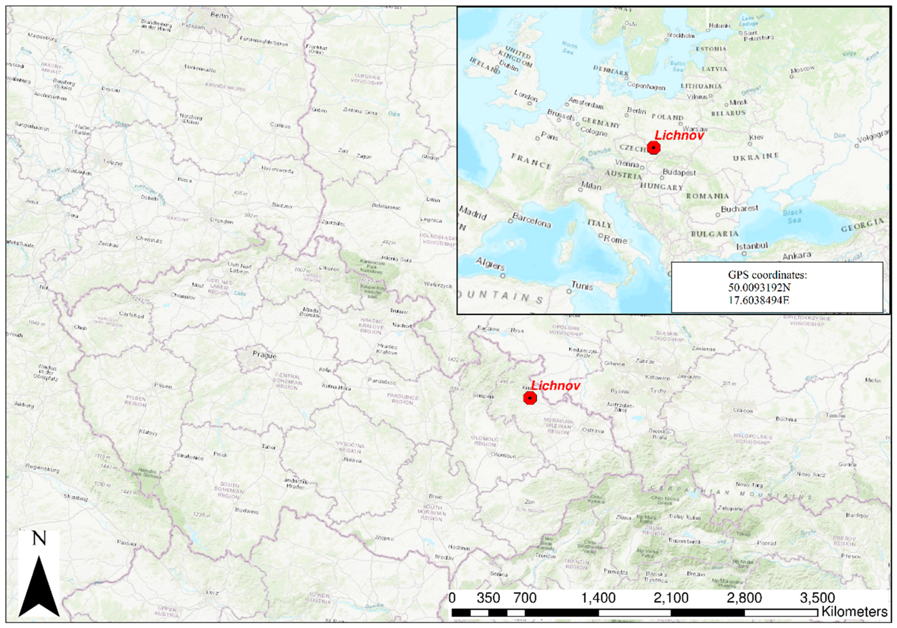During extreme floods in 1997, 2002, and 2010, dozens of collapsed small dams were reported [4]. Therefore, dam break studies, including dam-break flood propagation modeling are also carried out for systems of small dams. An example of the application of dam break modeling to a cascade of small earthen dams is presented in this case study of the Čižina River in the Czech Republic.

For Emergency Action Plans, it is necessary to specify the characteristics of the dam-break flood and the extent of the endangered area. The knowledge concerning such flood-prone areas aids in the development of warning systems and evacuation plans. Various hydraulic and sediment transport models can be used for this purpose [5,6,7,8].

Numerous authors have dealt with the issue of dam breach modeling. In the 1970s, Cristofano [1] collected data from historical failures of earth-fill dams occurring up to 1965, based on which he performed a simulation of the onset of erosion. In the early eighties, the BRDAM model [9] was used to simulate the erosion of an earth dam in the case of overtopping or internal erosion. Subsequent authors [10] improved the model by specifying the place of origin, simulating the erosion at the lowest point of the dam crest. The surface erosion proceeding on the downstream slope was modeled. The model used continuity equations, sediment transport equations, and equations for the formation of the dam breach opening via surface erosion. Nogueria [11] subsequently presented a 1D model using Saint–Venant’s equations to describe unsteady flow and Exner’s, Meyer–Peter, and Muller’s formula for sediment transport. Almost at the same time, Fread [12] published the numerical models BREACH and Dam Break Forecasting model (DAMBRK), which allowed the simulation of a dam breach via both overtopping and internal erosion, including the effect of lateral slope due to a landslide. That same year, Fread [13,14] introduced the National Weather Service dam-break flood forecasting model (NWS DAMBRK) numerical model. It was based on complex hydrodynamics and erosion processes, and marked the first inclusion of soil strength characteristics within such a model. An improved model, BEED [15], also simulated erosion processes during a dam break. The existing empirical and numerical procedures were summarized by Wahl [3], who proposed an inventory for the development and further improvement of numerical models. These works were followed by Říha and Daněček [16], Tingsanchali, and Chinnarasri [17], and others using different approaches to derive a breach outflow hydrograph using different erosion formulae. Later, a group of authors at HR Wallingford [18,19,20] developed the numerical model named HR BREACH now Embankment Breach (EMBREA), which allows the input of parameter intervals characterizing the material properties of soils, and then performs Monte–Carlo simulations to find the most unfavorable result of the simulation. In 2005, Hanson developed the Simplified Breach Analysis (SIMBA) now Windows Dam Analysis Modules (WINDAM) model for the Agricultural Research Service and Natural Resources Conservation Service in the US [21]. Currently, the newest version of the program (WINDAM C) is able to model the overtopping and internal erosion of embankment dams, as well as head-cut erosion and the failure of protective layers. In 2012, the AREBA software was developed by [22]. The software is capable of simulating a dam break via overtopping or internal erosion in homogeneous and composite embankments. The numerical module Breach_Macchione [23] was adopted to the code Basement in 2012 by Voltz et al. [24]. The model is based on the application of two-dimensional shallow-water equations to breaching processes occurring in non-cohesive embankments due to overtopping. Wu [25] developed A Simplified Physically-Based Dam/Levee Breach (DL Breach), which simulates dam and levee breaching via overtopping and internal erosion in homogeneous and composite materials. It can simulate the failure of cover surfaces and can perform Monte–Carlo simulations. Recently, researchers have incorporated simplified modules into River Analysis System (HEC-RAS), A modelling system for Rivers and Channels (MIKE11 DB), WOLF, Rubar 20TS, and other software for modeling water flow in inundation areas [5,26,27,28]. Recent work by King and Simonovic [29] presents a deterministic Monte–Carlo simulation concept used for the assessment of dam safety management control.

In the case of the breaching of dams in a cascade, the resulting dam-break flood depends on numerous factors like the rate of breaching of the upper dam, the ratio of the volumes of the reservoirs in the cascade, and the ability of the lower reservoirs to attenuate the flood wave. The distance between individual reservoirs and the characteristics of the floodplain are also important factors. Therefore, the dam-break flood routing along a cascade of reservoirs may vary according to the failure mode of the uppermost dam and to the current water level and free volume of the reservoirs in the cascade. Usually, the most unfavorable scenario is used for Emergency Action Plans. Only a few studies deal with dam breaks in a cascade of reservoirs [30,31,32,33]. Liu et al. [31] describe a procedure for the numerical simulation of a dam breach due to overtopping in a cascade together with risk analysis. This includes the 1D flow open channel modeling of flood propagation. Stoyanova and Coombs [32] use the methodology applied in the AREBA software. Both simple two-reservoir and more complex four-reservoir cascade scenarios are dealt with. Cai et al. [30] applied Bayesian networks for the quantification of the flood risk due to dam breaks in a cascade. Studies [30,31,32,33] focused on large dams with the possibility of outflow discharge regulation.

The lessons learned during past extreme floods [2,4,34] show that on average, about ten small dams fail in the Czech Republic during extreme flood events and that such dams are more vulnerable to breaching than large dams, which is primarily due to their insufficient spillway capacity. As a rule, such schemes have a flood attenuation volume, which is relatively small when compared to the volume of the arriving extreme flood. Their fixed spillways usually have a limited capacity due to the low importance of the dams.

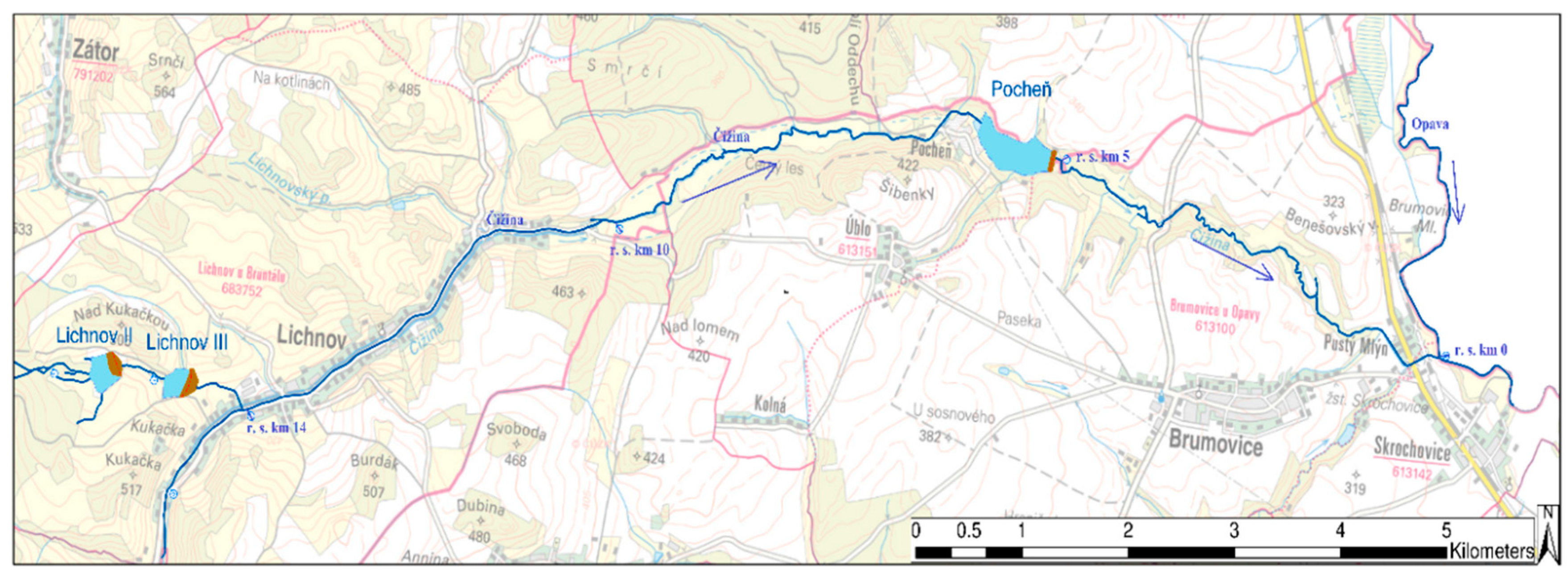
This study aims to fill a gap in the research concerning the breaching of small embankment dams in a cascade. It deals with a cascade of three relatively new small embankment dams in the Čižina River catchment in the Moravian–Silesian Region of the Czech Republic. One of the aims was to demonstrate the effect of the distance between dams on dam-break flood attenuation. In our case study, the two upper reservoirs are quite close to one another, while the lower one is located more remotely downstream along the Čižina River. A complete set of technical data about the dams was available. The lowest dam, Pocheň, has already experienced overtopping twice but it resisted in both cases and did not fail.

Based on the results of the analysis, typical dam-break flood routing characteristics are summarized for a cascade of small dams. The method proposed in the study may be used for the development of Emergency Action Plans containing dam break and flood routing analyses for the affected area below a dam. The results of such analyses contain flood arrival times and maps with flood zones where water velocities and depths are included.

2. Case Study

2.1. Study Area

The case study covers an area of the Čižina River catchment in the Moravian–Silesian Region of the Czech Republic (Figure 1) that extends for about 103 km².

In the catchment area, three small reservoirs named Lichnov II, Lichnov III, and Pocheň are arranged in a cascade (Figure 2). The cascade was selected because the distance between the dams differs significantly, allowing the demonstration of the impact of distance on dam-break flood attenuation. The two upper reservoirs are quite close to one another, while the lower one (Pocheň) is about 15 km downstream from the Lichnov III dam. A complete set of technical data about the dams was available. The lowest dam, Pocheň, has already experienced overtopping twice, but it resisted in both cases and did not fail.

2.2. Description of the Small Dams

The main characteristics of the studied dams are described in

Table 1. Description of the small dams.

Basic Characteristic of Dam	Lichnov II	Lichnov III	Pocheň	Units
Dam height	14.6	10	8.5	(m)
Crest width	5	4	4	(m)
Upstream slope	2	3	3	(1/X)
Downstream slope	2.8	2.6	2.3	(1/X)
Material classification	Gravel clay	Loam gravel	Gravel clay	(–)

.

The Lichnov II dam is located about 1 km above the village of Lichnov on Tetřeví Stream, which is a tributary of the Čižina River. The dam was built in 2015. The main purpose of the reservoir is to provide flood protection to the villages downstream. The dam is homogenous and is made of sandy to gravelly clay. The maximum height of the dam above the local terrain is 16 m, and the dam crest is 5 m wide. A longitudinal section along the dam crest is shown in Figure 3, while a typical cross-section is displayed in Figure 4. The dam crest elevation at the left abutment is 0.85 m lower than the dam crest due to the presence of an emergency spillway. This place where overtopping may start, and water flows rapidly along the downstream slope was considered to be the potential point of origin of a breach due to overtopping. At the toe of the right abutment, extensive leakage through disintegrated colluvial soil below the base of the dam was identified via technical surveillance during the first trial filling of the reservoir. It is considered that there is a threat of backward erosion piping and a possible breach at this location.

The length of Tetřeví Stream between the Lichnov II and Lichnov III reservoirs is relatively small, about 500 m. The valley is relatively steep and narrow and is covered by forest and meadows.

The small detention dam Lichnov III is located approximately 400 m upstream of the village of Lichnov. It was built in 2018. Its purpose is to protect the village and to transform incoming flood waves from the Lichnov II dam and from the area adjacent to the reservoir. The dam body is homogeneous. It is made of sandy to gravelly clay and is very similar to that of Lichnov II. The dam height is about 12 m; see Table 1 for its main characteristics and parameters. As a dam-break flood arriving from the Lichnov II dam would be sudden, it is not probable that a gradually evolving piping process would develop, and so only overtopping was considered as a potential failure mode. The place of overtopping was similar to that of Lichnov II, i.e., at the auxiliary crest spillway at the left abutment (Figure 5).

About 600 m downstream of the Lichnov III dam, Tetřeví Stream flows into the Čižina River, which passes through the village of Lichnov. Numerous civil structures such as bridges and culverts are located there, and the area along the 3.5 km long river reach is urbanized with numerous buildings. Further, on the downstream of the village, the Čižina River continues into a region of fields and meadows covered with trees. This section of the Čižina River stretches for about 6 km, after which the river enters the Pocheň reservoir.

The small dam named Pocheň is located on the Čižina River about 5 km upstream of its junction with the larger Opava River. The Pocheň dam was built between 1973 and 1975 as a source of water for agricultural activities in nearby areas. During the extreme flood event in the year 1996, the dam was seriously damaged by overtopping but not breached. Due to this damage, reconstruction of the dam body took place, and the spillway capacity was improved over the following years. The dam height is about 9.5 m, and the dam is constructed from local gravelly clay. The geodetic survey indicated the lowest crest elevation is approximately in the middle of the crest length (see Figure 6). Due to the short duration of the extreme load, a progressive piping failure would not develop, and so only the overtopping failure mode was taken into account.

Downstream of the Pocheň reservoir, the Čižina River passes through an area of forest, flows below several road and railway bridges, and then enters the Opava River close to the village of Skrochovice.

3. Methods

Both empirical formulae and comparison with real incidents were applied for the first preliminary estimates of the dam break peak discharges. The obtained values provide an idea about the range of the peak outflows and provide a general framework for numerical modeling. Due to the lack of relevant incidents and reliable data from real breached dams, these equations suffer from a great deal of inaccuracy and are mainly useful for the preliminary estimation of parameters, which can then be determined more precisely by numerical models.

The dam break simulation was carried out using the numerical model of breaching due to overtopping and internal erosion (the latter phenomenon at the uppermost dam only), which is normally applied to individual dams. The peak discharges were compared with the results of empirical formulae and with real cases involving the failure of small dams.

Two-dimensional shallow-water flow hydraulic models were applied for the simulation of the dam-break flood propagation into the areas between the dams. The flow and erosion parameters were searched via Monte–Carlo random sampling to achieve the highest peak outflow discharge below the dam.

3.1. Empirical Formulae

In order to obtain an initial idea about the peak discharges, published empirical formulae were applied. This approach is the simplest but least accurate way of predicting dam breach parameters. In dam-break simulations, direct calibration of models is usually impossible. One of the methods of verifying numerical models is to compare the modeling results with the outputs of retrospective studies of real incidents and failures. Unlike, e.g., hydrological floods, there is a lack of dam-break calibration data worldwide due to a lack of relevant incidents and reliable data from real breached dams. The empirical formulae discussed in this study (

Table 2. Summary of formulae used for estimating the peak breach outflow Q_b.

Author, Reference	Formulae for Qb *) (m3/s)
Holomek, Říha (2000) [35]	$Q_b=m\sqrt{2g}\left[b{H}_k{}^{1.5}+0.4\frac{B-b}{h_d}{H}_k^{1.5}\right]$
The following breach dimensions can be used:
USACE (1980) [36]	$b=3h_d\hspace{1em}\&\hspace{1em}B=5h_d$
ICOLD (1974) [37]	$b=1.6h_d\hspace{1em}\&\hspace{1em}B=3.6h_d$
Šimek (1988) [38]	$b=1.2h_d\hspace{1em}\&\hspace{1em}B=3.2h_d$
Froehlich (1995a, 1995b) [39,40]	$Q_b=0.607V_w{}^{0.295}{h}_w{}^{1.24}$
Webby (1996) [41]	$Q_b=0.0443\cdot g^{0.5}{V}_A^{0.367}{h}_w^{1.40}$
Bulletin 111 (1998) [42]	$Q_b=0.07{\left(g{h}_d\right)}^{0.5}{h}_d^2{\left(\frac{V_b}{h_d^3}\right)}^{0,5}$
Vischer, Hager (1998) [43]	$Q_b=1.25·{10}^{-2}\frac{H_a}{h_d}\sqrt{g{B}_a^2{h}_d{}^3}$

*) An explanation of the variables can be seen in the section “List of symbols”.

) are based on such real cases. It is true that statistical analysis is difficult due to the heterogeneity, inaccuracy, and scatter of the dam break data when subjected to regression analysis. However, the published empirical formulae and the analogy method are frequently used in dam break analysis for the comparison of real incidents with the results of numerical analysis.

One of the aims of this study was to demonstrate the difference between a single dam break and a cascade when applying empirical formulae.

3.2. The Analogy Method

A more reliable peak breach outflow may be derived via the comparison of data from real incidents at dams with similar characteristics (dam type, height, reservoir volume) to the studied dam. The data may be obtained from publications and extensive dam failure databases (both national and international) [2,3,34,42,44,45]. In

Table 3. Summary of the characteristics of the real breached dams and the studied dams.

Cases	Dam Name	Dam Height (m)	Reservoir Volume (ths. m3)	Crest Width (m)	Breach Width (m)	Peak Outflow (m3/s)
Real cases	Metly	8.50	1930	4.0–6.9	35.0 + 15.0 *)	550
	Velký Bělčický	6.70	1063	7.4	42.0	600
	Buffalo Creek	14.00	483.5	107.0	148.0	1416
	Kelly Barnes	11.50	505	6.1	6.7	680
Studied dams	Lichnov II	14.60	400.6	5.0	-	-
	Lichnov III	10.00	117.9	4.0	-	-
	Pocheň **)	8.50	780	4.5	-	163

*) Two breach openings. **) The dam was not completely breached.

, dams similar to those studied are mentioned together with basic relevant characteristics (see also Chapter 2).

3.3. Embankment Dam Breach Modeling

A simple parametric model based on hydraulic and transport modules was used for the simulation. The tailor-made code was developed in MATLAB software to allow the dam breaching process to be modified easily according to local conditions and the failure mode.

The main output of the dam break analysis is the outflow hydrograph Q(t), which results from the failure. The following steps were performed before the modeling took place.

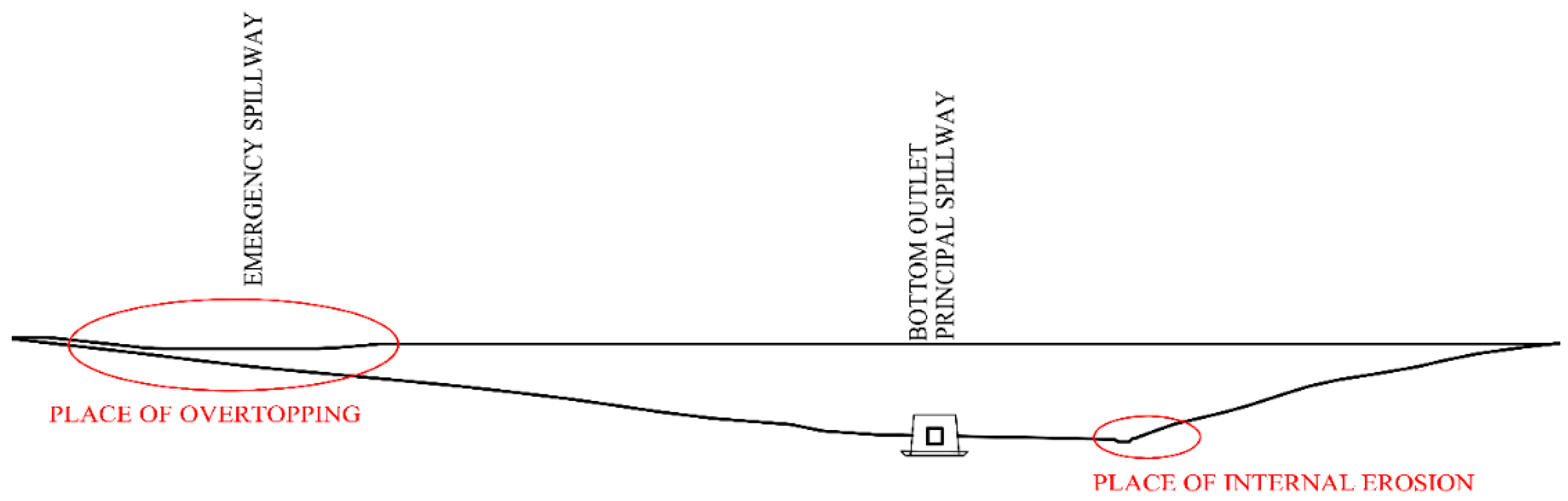
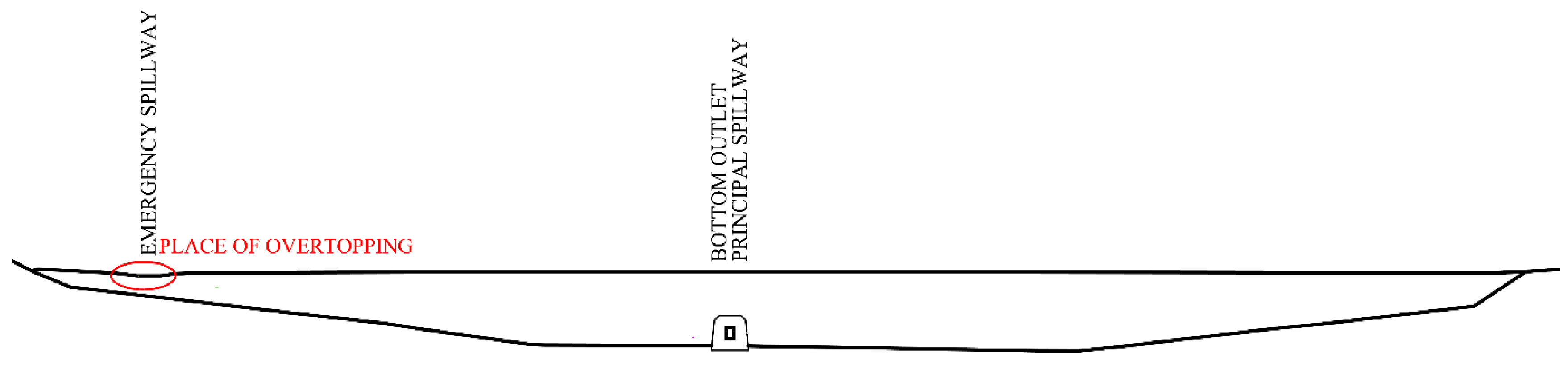
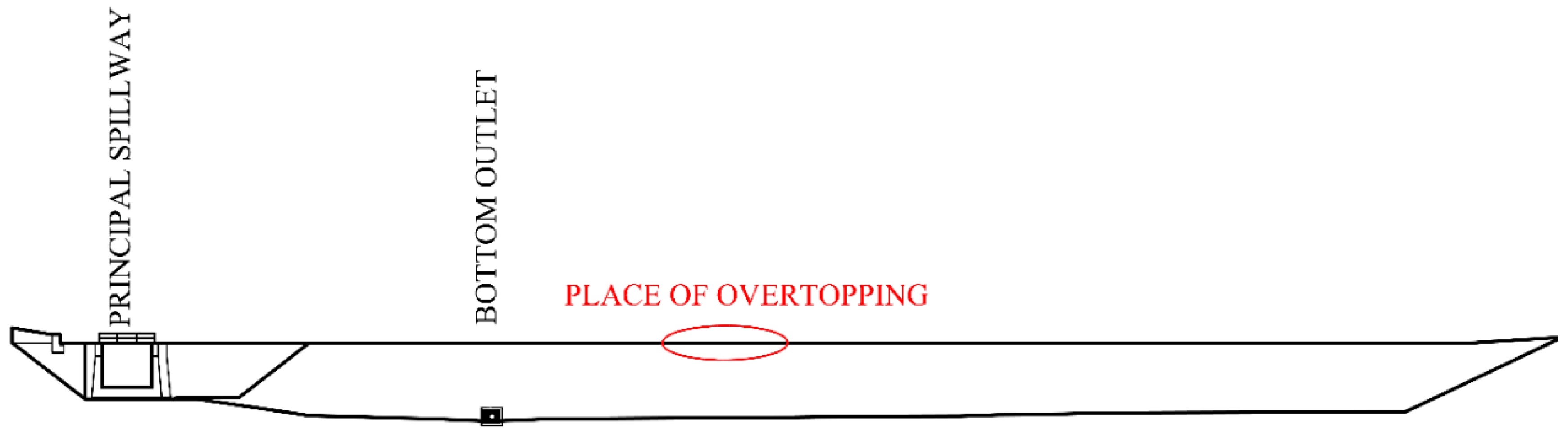
A careful investigation was performed with regard to the dam type and structure (material, emergency spillway position, dam surface, type of pavement on the dam crest, etc.), as well as the local geological conditions (subbase material, material discontinuities).

The probable place of failure initiation was located; for an overtopping failure, the place with the minimum dam crest or auxiliary spillway height was chosen. For a piping failure, the location with the weakest subbase providing the highest seepage was chosen.

• The shape of the dam break opening was rectangular for overtopping and circular for piping.
• The flood hydrograph Q_in (t) entering the reservoir was provided by Czech Hydrometeorological Institute.
• The bathymetry of the reservoirs was taken from a geodetic survey of the reservoir area.
• The initial reservoir water level H₀(t) was taken from the dam operation manual. It corresponds to the live storage water level.

The following relation between the reservoir inflow, outflow, and a change in water level holds:

$$\frac{\mathrm{d}V}{\mathrm{d}t}=Q_{in}\left(t\right)-Q_b\left(H\right)-Q_f\left(H\right)$$

(1)

where V is the reservoir water volume (m³), t is time (s), Q_in is the reservoir inflow (m³/s), Q_b is the breach outflow (m³/s) (in the following text, Q_bo denotes overtopping discharge and Q_bp piping discharge), Q_f is the outflow through appurtenant works (outlets, spillways, etc.) in (m³/s), and H is the elevation of the water level (m a. s. l.).

The outflow through the appurtenant works governed by the reservoir water level was calculated using equations taken from standard dam hydraulics [46]. The equations used and related coefficients were determined according to the arrangement of the hydraulic structures.

3.3.1. Overtopping

In the case of dam overtopping, the breach was approximated using a 1D model. The breach started at the lowest point of the dam crest, where the first overtopping occurred. The overtopping width along the dam crest was suggested as an initial breach width, b₀. The shape of the breach opening was approximated by a rectangle, and the erosion progress was applied in both the downward and the lateral direction. The water moving along the downstream slope was assumed to exhibit quasi-steady uniform flow [3,13,45] with no submergence from the downstream side. The resistance of the dam body against the surface erosion was evaluated with respect to the water flow velocity at the downstream slope, with non-scouring velocity being used for the evaluation. Parallel uniform gradual backward erosion of the downstream slope was assumed [13]. The angle of the downstream slope and the width of the dam crest were set as input parameters, along with hydraulic parameters such as the discharge coefficient m, Manning roughness n, and the non-scouring velocity v_ns and erosion parameters of the soil α₁ and α₂, together with initial conditions (see below).

The breach outflow during overtopping Q_bO was calculated using an overflow formula for a rectangular broad crested weir [47]:

$$Q_{bO}=mb\sqrt{2g}{\left(H-Z\right)}^{1.5}$$

(2)

where m is the weir coefficient, b is the width of the breach opening (m), g is the acceleration due to gravity (m/s²), and Z is the breach bottom elevation (m a. s. l.).

Using the overtopping discharge obtained from Equation (2), the water depth h_f and velocity v_f along the slope was derived from the Chezy equation [47]:

$$h_f={\left(\frac{Q_{b0}n}{b\sqrt{sin\beta }}\right)}^{0.6}$$

(3)

$$v_f=\frac{\sqrt{sin\beta }}{n}{h}_f^{0.67}$$

(4)

where n is the roughness of the downstream slope, and β is the downstream slope angle.

At the moment, when the flow velocity along the slope exceeds the non-scouring velocity v_ns (the value is an input parameter), erosion occurs and the breach starts to increase in width and depth [34]:

$$\frac{\mathrm{d}Z}{\mathrm{d}t}=-{\alpha }_1{v}_f,\mathrm{for}{v}_f>v_{ns}$$

(5)

$$\frac{\mathrm{d}b}{\mathrm{d}t}={\alpha }_2{v}_f,\mathrm{for}{v}_f>v_{ns}$$

(6)

where α₁ and α₂ are erosion parameters.

Initial conditions specify the reservoir water level H₀, the lowest dam crest elevation Z₀, and initial overtopping width b₀ at the beginning of the solution (t = t₀). The set of Equations (1) to (6) was solved numerically using the Newton method with a small-time step Δt = 1 s.

3.3.2. Piping

For the piping model, a circular opening with a constant leakage pipe diameter and constant shear stress and hydraulic gradient along the pipe were assumed [19,20,21,22,28,48]. The input parameters were the length of the pipe L, the initial reservoir water level H₀, the elevation of the pipe outflow H_outflow, the critical shear stress along the walls of the pipe τ_c, the soil erodibility C_e, the initial pipe diameter D₀, and absolute roughness Δ.

The outflow through the pipe Q_bP and average water velocity v_pip in the pipe were determined using pipe hydraulics [47]:

$$Q_{bP}=\frac{1}{\sqrt{\alpha +\lambda \frac{L}{D}}}S\sqrt{2g\left(H-H_{outflow}\right)}$$

(7)

$$v_{pip}=\frac{Q_{bP}}{S}$$

(8)

where α is the kinetic energy (Coriolis) coefficient, L is the length of the pipe (m), D is the pipe diameter (m), λ is the friction loss coefficient, S is the pipe cross-sectional area (m²), and H_outflow is the pipe outflow elevation (m a. s. l.).

Using the water velocity in the pipe, the average hydraulic gradient along the pipe I_E and shear stress τ acting on the pipe walls were obtained:

$$I_E=\lambda \frac{1}{D}\frac{v_{pip}^2}{2g}$$

(9)

$$\tau =\rho g\frac{D}{4}{I}_E$$

(10)

where ρ is the water density. When the critical shear stress τ_c on the pipe wall was exceeded, erosion and an increase in the pipe diameter initiated. The rate of erosion $\dot{\epsilon }$ and the change in pipe radius dr were determined according to equations suggested by Wan and Fell [48]:

$$\dot{\epsilon }=C_e\left(\tau -{\tau }_c\right)$$

(11)

$$\mathrm{d}r=\frac{\dot{\epsilon }}{{\rho }_b}\mathrm{d}t$$

(12)

where $\dot{\epsilon }$ is the rate of erosion (kg/s/m²), C_e is the coefficient of soil erosion (s/m), ρ_b is the bulk density of the eroded soil (kg/m³), and r = D/2 is the pipe radius.

The initial reservoir water level H₀ and initial pipe diameter D₀ are the initial conditions. As in the case of overtopping, the solution of Equations (1) and (7) to (12) was carried out using the Newton method with a very small-time step of Δt = 1 s.

During the solution, the relation between the pipe diameter and the thickness of the roof of the conduit (overburden) was checked. After the pipe diameter exceeded the overburden thickness, it was assumed that the soil layer above the opening collapsed and the process continued similarly as in the case of overtopping. The width of the breach opening corresponded to the pipe diameter at the instant of the overburden collapse, while the breach bottom was assumed to be at the top of the seepage pipe at the instant of the collapse.

3.3.3. Optimization Procedure

Most of the input parameters in both scenarios are rather uncertain, and realistic intervals of their values were estimated from literature sources and real cases [3,41]. The combination of parameter values from their intervals may result in significant differences in outflow hydrographs and peak outflow discharge. In order to obtain the least favorable result with the highest peak outflow, the “optimization” of the parameters mentioned in

Table 4. Intervals of parameters for the Monte–Carlo sampling procedure.

Overtopping.			Piping
Parameter (units)	Minimum	Maximum	Parameter (units)	Minimum	Maximum
n (s/m1/3)	0.025	0.035	d0 (mm)	5	100
α1 (-)	0.0002	0.0030	Δ (m)	4.56 × 10−4	9.58 × 10−4
α2 (-)	0.0002	0.0015	τc (Pa)	1.3	64
vns (m/s)	1.8	3.0	Ce (s/m)	1.38 × 10−3	4.24 × 10−3

was performed via the Monte–Carlo sampling procedure [49].

The most influential parameters for the optimization were determined based on the equations governing the breach outflow discharge. The shape of the dam break hydrograph and namely the peak outflow discharge is generally governed dominantly by the size of the breach opening and the water level in the reservoir (Equations (2) and (7)). Crucial variables influencing the shape and size of the breach opening are the erodibility parameters (Equations (4)–(6) for overtopping and Equations (8) and (12) for piping). The reservoir water level is determined via level pool routing through the reservoir, Equation (1), and depends on the reservoir bathymetry V(H), the inflow flood hydrograph Q_in, the capacity of the appurtenant works Q_f, and the breach outflow Q_b. The importance of the mentioned variables was proved by sensitivity and statistical analyses carried out in a previous study [50]. In this study, the members in Equation (1) were not subject to optimization as they were “prescribed” by the Czech Hydrometeorological Institute (inflow hydrograph), by the reservoir bathymetry, and by the capacity of the spillway.

For each dam, about 10 thousand simulations were carried out using parameter values obtained from random sampling. A uniform probability distribution was used for each parameter. As a result, a “sub-optimal” scenario was found after a reasonable amount of computational time with sufficient accuracy when compared to other simplifications adopted (the mathematical model, for example). The scenario with the highest peak outflow was used for further processing.

3.4. Dam-Break Flood Routing

The dam-break flood routing between reservoirs was simulated using a two-dimensional (2D) model based on shallow-water flow equations [8]. The solution was performed using the commercial code HEC-RAS v. 5.0.7 [5]. As the model used is standard and the procedures are routine, the model is not described here in detail, and the authors refer those interested to the available literature [5,46]).

The inputs for the calculation were the topology and geometry of the area between the dams taken from a digital model of the terrain (DTM). Civil structures were assumed to be fixed, with no damage suffered due to the flow of water.

The upstream boundary condition was represented by the dam breach flood hydrograph and hydrological flood hydrographs at contributing local streams. The initial condition was set as a stream discharge and water level corresponding to a 20-year return period, which corresponds approximately to the bank-full capacity of the streams.

4. Simulations and Results

First, the peak outflow from the dams was estimated using empirical formulae (Table 2) based on the dam and reservoir characteristics (Table 3). A comparison with real dam failures was also performed.

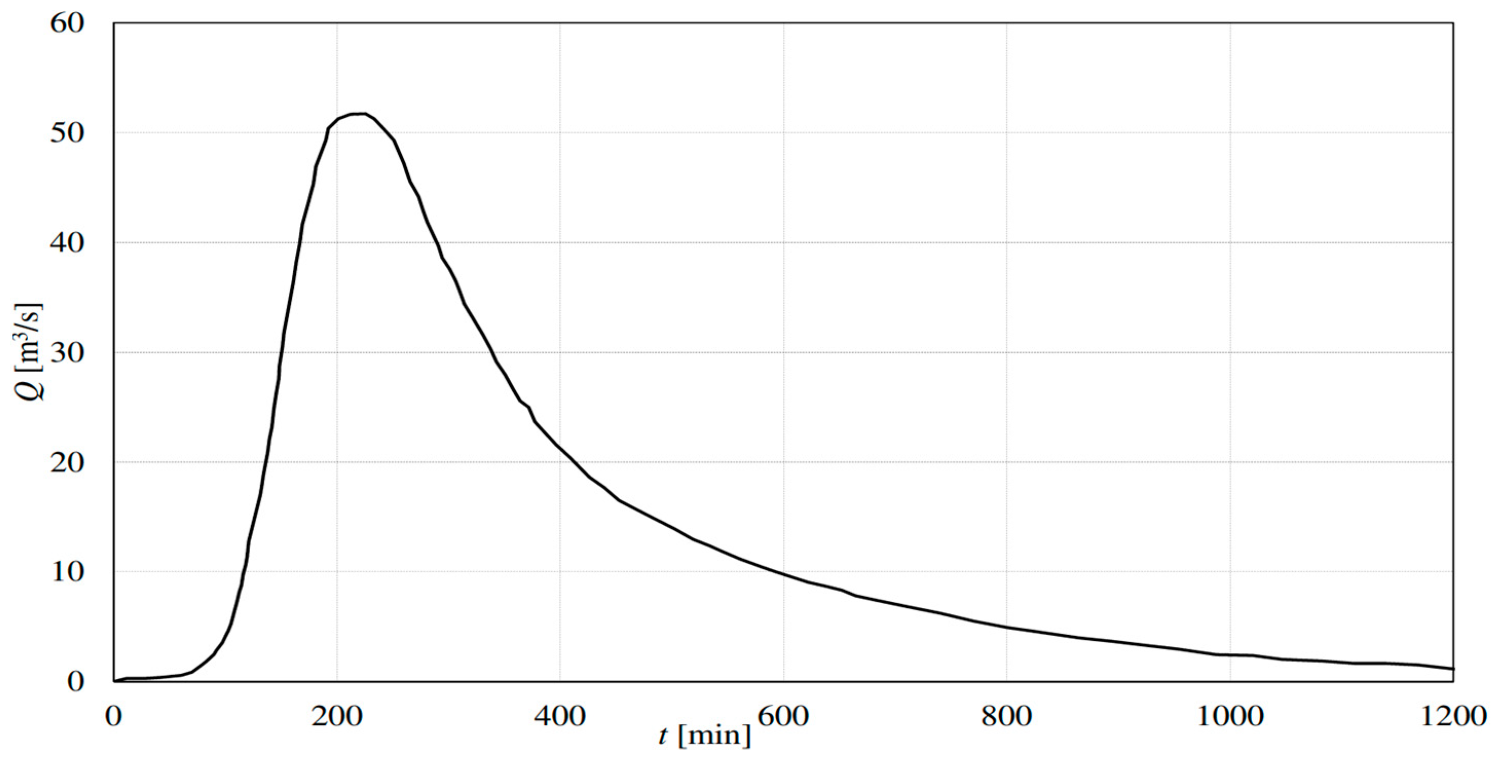
The numerical simulation started from the uppermost dam, Lichnov II. From an analysis of hydrological and empirical data, a check flood inflow hydrograph from the area upstream of Lichnov II was derived by the Czech Hydrometeorological Institute (Figure 7), providing a peak discharge of 50 m³/s. This approximately corresponds to the outflow of the largest experienced rainfalls at small river basins in the Czech Republic (more than 200 mm/day) during the floods in the years 1996, 1997, and 2010 at relatively small catchments with areas of 5 to 10 km².

The runoff from the larger catchment area between the reservoirs at the time of the dam break events corresponds to a flood with a 20-year return period. This assumption is also based on past experience from real floods at catchments with areas of 50 to 60 km². This also corresponds to the capacity of related streams in smaller urban areas.

The dam break study proceeded from the upstream reservoir in the downstream direction in five steps containing level pool routing:

-

through the Lichnov II reservoir (simulation of the dam breaching due to both overtopping and piping),

-

between Lichnov II and Lichnov III,

-

through the Lichnov III reservoir (simulation of the dam breaching due to overtopping),

-

between Lichnov III and Pocheň,

-

through the Pocheň reservoir (simulation of the dam breaching due to overtopping).

In order to achieve the worst-case scenario of dam breaching, in which the maximum peak outflow occurs from the collapsed dams, parameter optimization was carried out. The optimization was conducted using the parameters shown in Table 4, with their realistic intervals adopted from the available literature [2,3,37,40,45,50].

A summary of the final input values, including the final parameters obtained from the optimization procedure, is listed in

Table 5. Summary of inputs for the numerical model.

Inputs for the Numerical Model (units)	Notation	Input Overtopping and Piping Values
		Lichnov II	Lichnov III	Pocheň
Initial water level in the reservoir (m a. s. l.)	H0	444.30	424.00	315.90
Dam crest elevation (m a. s. l.)	CL	453.50	425.30	317.50
Dam bottom elevation (m a. s. l.)	BL	442.00	414.50	308.00
Bottom outlet axis elevation (m a. s. l.)	HSV	440.00	414.24	-
Auxiliary spillway crest elevation (m a. s. l.)	Haux	452.80	424.80	-
Initial elevation of the lowest point on the dam crest (m a. s. l.)	Z0	-	-	317.40
Discharge coefficient (-)	m	0.33	0.33	0.33
Initial overflow width at the auxiliary spillway/lowest point on the dam crest (m)	bspill	25	12	15
Non-scouring velocity (m/s)	vns	2.2	2	3.1 **)
Manning roughness coefficient of the downstream slope (s/m1/3)	n	0.031	0.032	0.030
Erosion parameter of the breach bottom (-)	α1	0.0007	0.0008	0.0002
Erosion parameter of the breach banks (-)	α2	0.0004 *)	0.0003 *)	0.00021
Initial pipe diameter (mm)	D0	5	-	-
Critical shear stress (Pa)	τc	1.3	-	-
Soil erodibility (s/m)	Ce	1.3 × 10−3	-	-
Elevation of the erosion pipe axis (m a. s. l.)	Houtflow	438.00	-	-
Length of the pipe (m)	L	74.5	-	-
Absolute roughness (m)	Δ	9.32 × 10−4	-	-

*) Lateral erosion in one direction. **) Determined from real incidents.

. The input values mentioned in Table 5 result in the maximum outflow discharge from the reservoirs during the breach event.

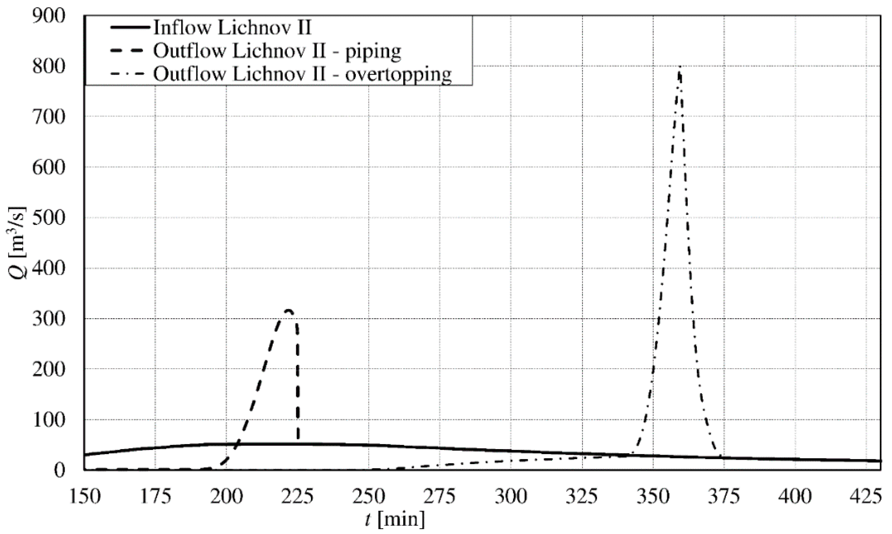
At the Lichnov II dam, both overtopping and piping failure were modeled. Figure 8 shows that the piping initiated approximately at the time of the peak inflow while overtopping occurred about 25 min after the inflow peak. The initialization phase at overtopping was followed by the gradual enlargement of the breach opening up to a final width of 68 m, which was reached about 125 min after the first overtopping as a result of intensive erosion only at the left side towards the central axis of the dam. A comparison of the modeled breach outflow hydrographs (Figure 8) shows that the peak discharge caused by the overtopping failure (802 m³/s) was more than 2.5 times higher than that caused by piping (316 m³/s). Therefore, the hydrograph from the overtopping failure was adopted for further analysis (Figure 8) of the cascade. This hydrograph provides a quite realistic duration for the breach event (approimately 30 min), which corresponded to that experienced during the breaching of small dams in the Czech Republic [34].

Most of the studied real dam failures exhibited peak discharges of 550 to 680 m³/s, except for in the case of the Buffalo Creek dam, which had 1416 m³/s (

Table 6. Summary results—peak breach outflows from Lichnov II, Lichnov III, and Pocheň.

Method of Determination		Maximum Breach Outflow Qbmax (m3/s)
		Lichnov II	Lichnov III	Pocheň
Comparison with real incidents at dams	Metly	550	550	550
	Velký Bělčický	600	600	600
	Buffalo Creek	1416	-	-
	Kelly Barnes	680	-	680
Empirical formulae	U.S. Army Corps of Engineers (1980) [36]	1763	1225	975
	ICOLD (1974) [37]	1078	754	595
	Šimek (1988) [38]	980	686	541
	Froehlich (1995a, 1995b) [39,40]	565	307	506
	Webby (1996) [41]	485	231	438
	Bulletin 111 (1998) [42]	578	224	628
	Vischer and Hager (1998) [43]	795	637	259
	Overtopping	802	841	557
	Piping	316	-	-

). Empirical formulae provide values, which are closer to the higher modeled discharge (485 to 1763 m³/s).

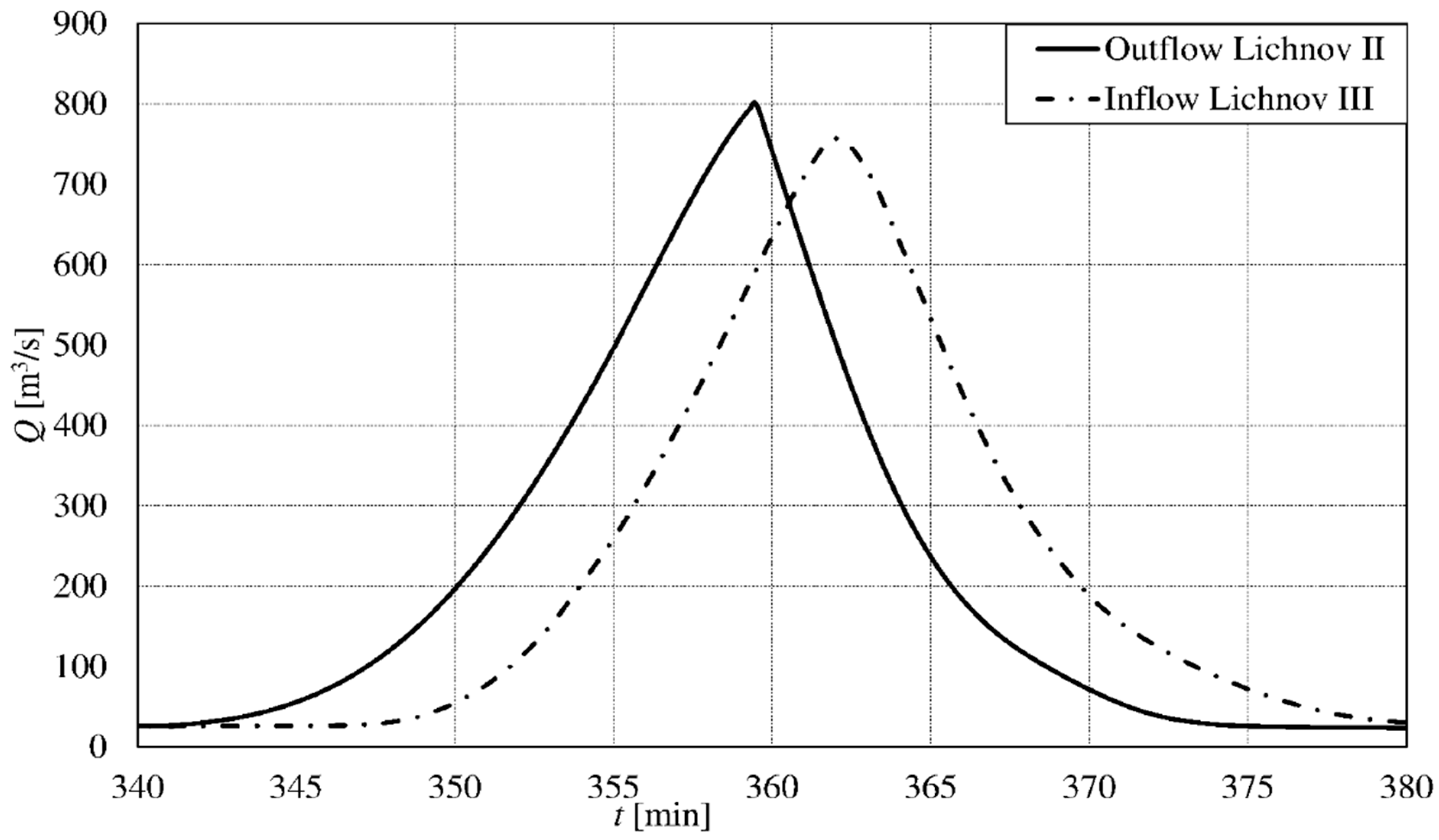
The flood routing between the Lichnov II and Lichnov III reservoirs along the 500 m long valley reach provided relatively small attenuation of the peak discharge from 802 m³/s to approximately 756 m³/s with a shift in the peak of about 3 min (Figure 9).

As mentioned above, the Lichnov III dam would be breached primarily by overtopping. The flood arrival was quite rapid (10 min), so the breaching started shortly after the rise in the reservoir water level. About 1 h was needed for the initiation of piping (Figure 8), and, therefore, the failure mode was primarily overtopping.

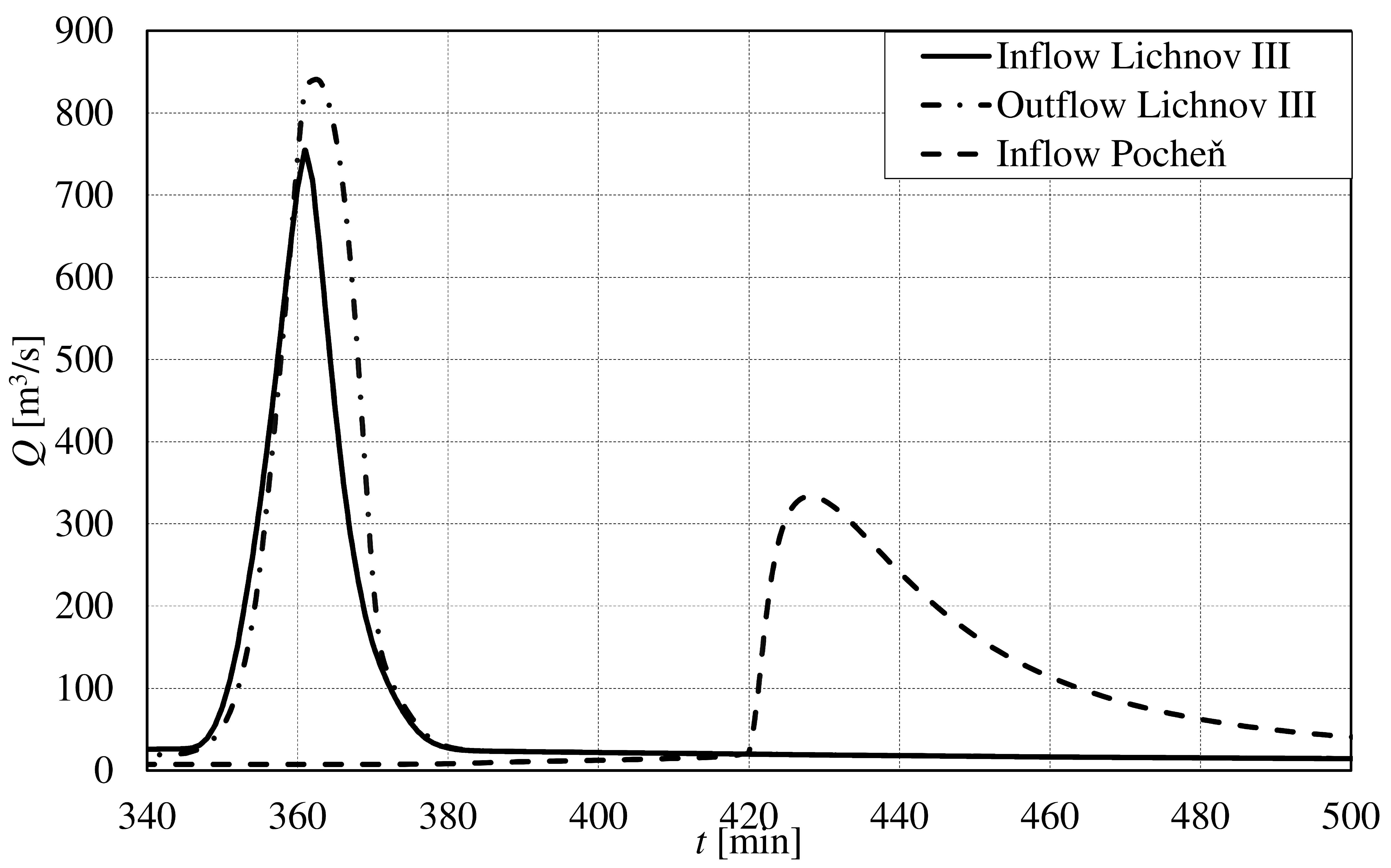
The modeled peak outflow of 841 m³/s from the dam occurred a few minutes after the arrival of the flood from the upper Lichnov II reservoir. The duration of the breach event was about 25 min, and the time at which peak outflow occurred is slightly after the time that peak inflow to the reservoir took place (Figure 10). The maximum breach width was 25 m. From Table 6 it can be seen that the range of values for the peak outflow derived from individual formulae varies from 231 to 1225 m³/s; the modeled peak outflow exceeds practically all calculated values (except for those obtained from USACE methodology). This could be attributed to the domino cascade effect that occurs when two dams are in very close proximity. Comparisons with empirical relationships and real dam failures may not be entirely relevant, as the difference between single and cascade dam breach peak discharge is about 50–55%. It should be noted that empirical equations correspond to single dam failure and do not take into account the domino effect.

If the Lichnov III dam were breached, the dam-break flood would arrive at the village of Lichnov fast, flooding most of the built-up area within 100 to 150 m of both banks of the Čižina River. Attenuation would be more significant below the village, where the floodplain of the Čižina River would be inundated over a 300 to 500 m wide area.

Flood routing along the remaining reach of Tetřeví Stream, and further on along the Čižina River resulted in a transformed hydrograph entering the Pocheň reservoir. From Figure 10, it could be seen that the peak discharge dropped from 841 m³/s to about 330 m³/s at the entrance to the Pocheň reservoir due to the attenuation along the 10 km long river valley between the Lichnov III and Pocheň dams (Figure 2). The time shift in the flood arrival time between both reservoirs is about 1 h.

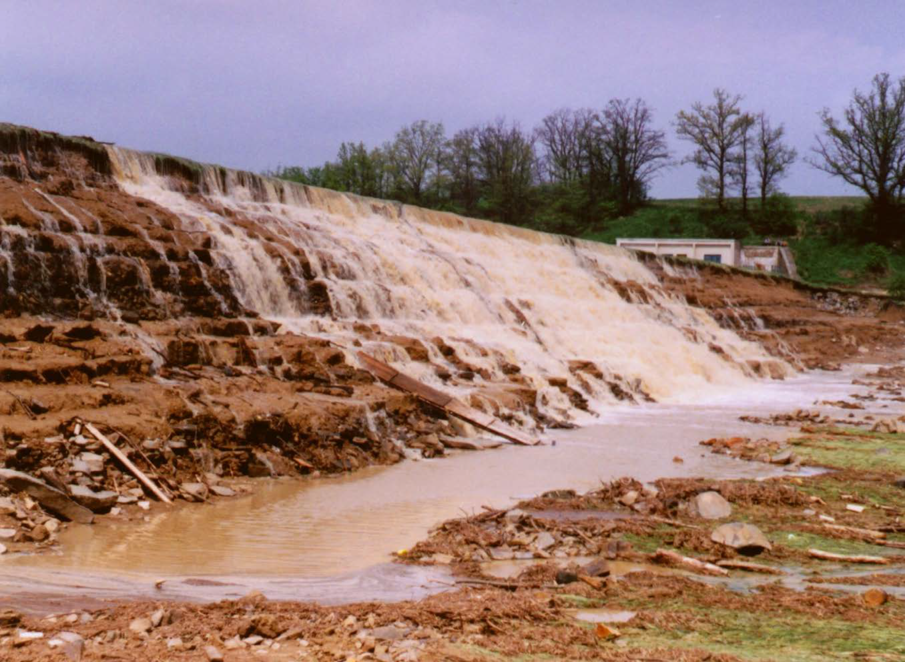
The input values of the erosion resistance characteristics for the simulation of the Pocheň dam breaching were verified using data from real overtopping events that took place during floods in 1977 and 1996 (Figure 11). They correspond to a non-scouring velocity of v_n ≈ 3.1 m/s, which was set in the calculation (it was not subject to optimization).

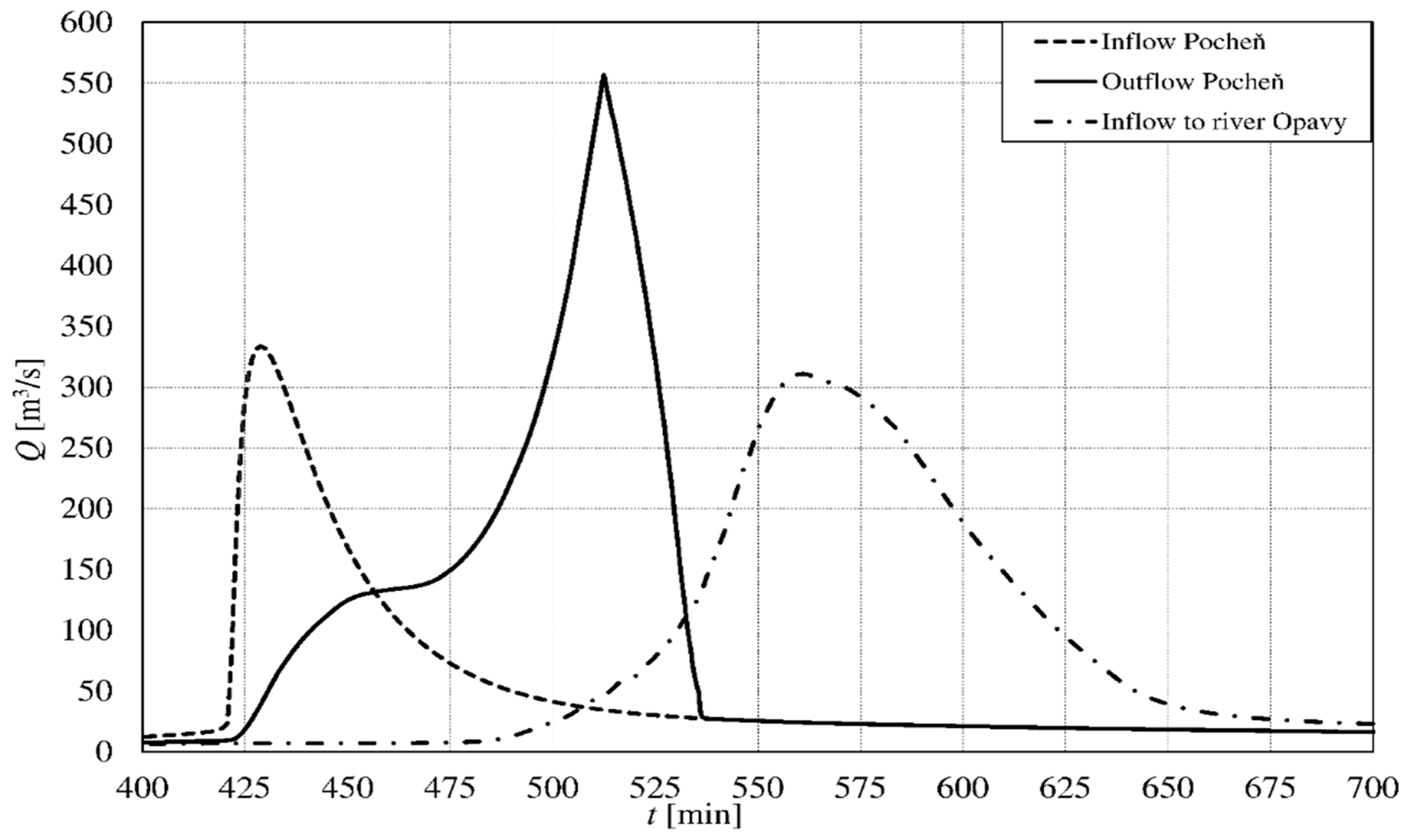
The resulting reservoir inflow and outflow hydrographs obtained by the simulation are shown in Figure 12. It can be seen that the peak outflow was delayed for approximately 1 h and 20 min after the culmination at the inflow. This time corresponds to the gradual filling of the flood attenuation reservoir storage, the overtopping of the relatively horizontal crest of the dam, and the slow development of the breach opening in the relatively resistant dam material. It can be seen that the peak inflow of 330 m³/s into the reservoir was increased by the breaching to a peak outflow of 557 m³/s, which is slightly higher than the average peak discharge obtained via comparative analysis and empirical formulae (Table 6). The minor difference between the simulated and empirical values was due to the characteristics of the cascade and other influences, including significant flood attenuation between the dams, the improved spillway capacity, and the rather higher dam body resistance against erosion.

The flood routing simulation continued down to the Opava River, which is located in a wide floodplain with road and railway embankments that create large “reservoirs” when flooded by the dam-break flood. This resulted in a relatively significant reduction of the 557 m³/s peak outflow from the Pocheň dam to approximately 310 m³/s at the junction with the Opava River (Figure 12). This peak discharge is lower than the 100-year return period discharge Q₁₀₀ = 352 m³/s of the hydrological flood in the Opava River downstream of the junction with the Čižina. As recommended in Guideline 14 [51], the dam-break flood simulation was terminated at the profile where the peak discharge induced by the dam break dropped below the 100-year hydrological flood discharge.

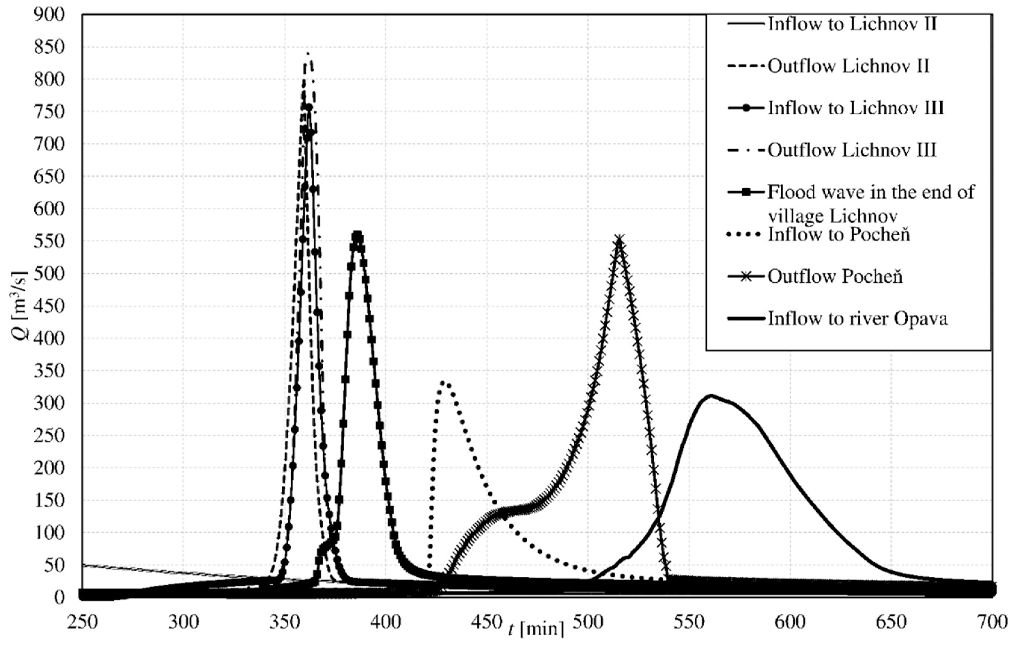
A summary of the simulations is shown in Figure 13, where the flood hydrographs are plotted starting with the initial hydrological flood that entered the Lichnov II reservoir (on the left) and induced the dam-break flood progression through the system of three reservoirs along the Tetřeví Stream and the Čižina River. In Table 6, the dam breach peak discharges obtained from simulations are compared with the results of the comparisons with real incidents and with data from empirical equations. The comparison indicates that the use of comparisons and empirical equations for a dam break in a cascade may be confusing, especially if the breached dams are very close to one another. These methods may be used for the comparison of the breach peak discharge failures at single dams, but with some caution due to the significant uncertainty involved.

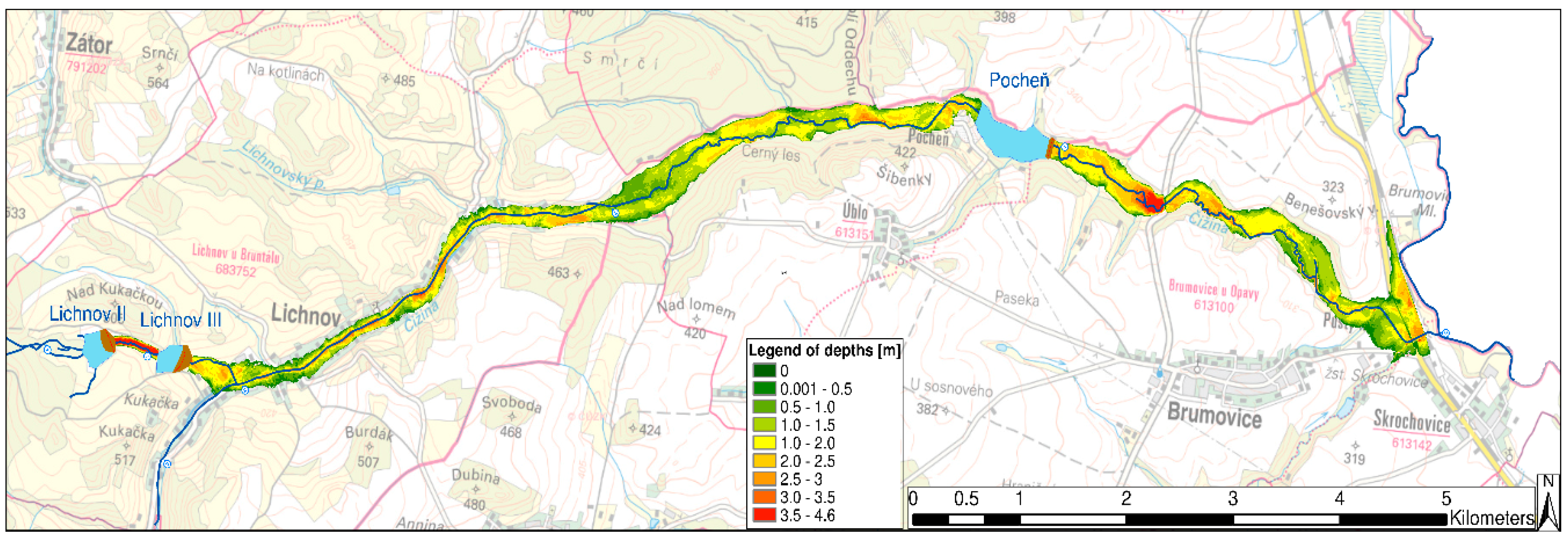
Figure 14 shows a map depicting the zone inundated by a dam-break flood corresponding to the worst-case scenario identified by Monte–Carlo optimization. The map displays the maximum water depth reached during the event.

5. Discussion

The simulation of a dam break in a cascade consists of two basic procedures, namely single dam-break analysis (Section 3.1, Section 3.2 and Section 3.3), and the analysis of the dam-break-induced flood between the dams (Section 3.4).

Basically, two failure modes—overtopping and piping—should be simulated at the uppermost dam. These modes are completely independent; they occur for different reasons at different places in the dam body, and at different times (Figure 3 and Figure 8). The initiation of piping is governed by the threshold hydraulic gradient when critical shear stress is exceeded. Therefore, piping usually starts at the rising limb of the flood hydrograph and progresses during the arrival of the flood peak at the maximum water level in the reservoir. This may happen before dam crest overtopping occurs. At the moment when the “roof” of the pipe becomes thin (here this is assumed to be when it is equal to the “pipe’s” diameter), the overburden collapses, and the simulation switches to the overtopping mode at the location of the original piping. This may result in a temporary drop in outflow during piping. The duration of the piping failure until the maximum breach opening developed was more than 1 h (Figure 8). The worst-case scenario of an overtopping failure occurred at the receding limb of the inflow hydrograph, at the moment when the reservoir was completely full, and critical velocity along the downstream slope was reached.

The optimization procedure showed that the outflow from a reservoir is predominantly governed by the size of the breach opening, and the reservoir water level in relation to the base of the breach opening. Thus, the peak outflow is limited by the location of the first overtopping, the morphology of the dam profile, and the erodibility of the dam material.

With large dams, the impact of the breaching of an upper dam on the failure risk of a downstream one is usually governed by the ratio between the released volume from the upper reservoir and the flood attenuation volume of the lower one. In the case of small dams, the flood attenuation volume is relatively small when compared to the volume of the arriving extreme flood, with the ratio varying between 1:10 and 1:25. The attenuation of peak discharge usually varies between 5–10%. Therefore, the attenuation effect of small reservoirs is not so important for dam break analysis in the case of a cascade of small dams. The capacity of the bottom outlets at small dams usually has a negligible effect on the flood passing through the reservoir and may be neglected.

At lower-lying small dams in a cascade where the reservoir only provides a limited attenuation effect, the rising limb is steep (Figure 9), and the increase in the reservoir water level is quite rapid (5–10 min). In the case of the scheme investigated here, the overtopping and breaching started shortly after the rapid increase in the reservoir water level. About 1 h was needed for the initiation of the piping, and, therefore, the expected failure mode was primarily overtopping. Therefore, the piping failure mode was not taken into account for the downstream dams.

The results of the presented study prove that flood attenuation between reservoirs located in close proximity to one another is practically negligible and that simplifications can be applied (Figure 9) [52]. Flood attenuation increases with the distance from the breached dam and follows an approximately exponential trend. Our results (Figure 13) correspond well with the results of parametric simulations published in [53], where the longitudinal slope, the dam-break flood volume, the width, and the “roughness” of the channel between the reservoirs are taken into account.

The empirical formulae tested in this study were derived using real collapses of single dams. When used for peak discharge estimation, empirical formulae derived for a single dam break should be applied carefully, as they may underestimate the peak outflow by up to 10% in the case of a dam cascade.

6. Conclusions

The paper describes the analysis of a dam break process in a cascade of small dams, including the simulation of flood routing along the adjacent streams. The aim is to fill a gap in the existing research concerning the breaching of small embankment dams in a cascade. This is a specific type of event which may differ from a dam break in a cascade of large dams, where the reservoir attenuation volume may play a significant role. The case study concerns an area along Tetřeví Stream and the Čižina River in the Moravian-Silesian Region of the Czech Republic. The area contains three small dams: Lichnov II, Lichnov III, and Pocheň. A simplified parametric model for piping and overtopping erosion with parameter optimization was used for the dam break simulations, while a standard 2D unsteady shallow-water flow model was applied for the flood in the areas downstream of each reservoir. As no calibration data were available, the comparison of the simulation results was carried out with the use of empirical formulae and by means of comparison with real small dam failures.

It is recommended that the solution for a dam cascade be divided into separate sequences corresponding to the dam breaching process and flood routing along the streams downstream of the dams. The location of the first overtopping and piping event should be identified based on the dam geometry, the arrangement of appurtenant works (namely the auxiliary spillway), observed leaks, etc. It is desirable to carry out at least a simplified optimization procedure, which guarantees that a combination of parameters providing the worst possible realistic scenario for the simulated event is obtained. When applying empirical formulae or comparison with real dam failures to a dam cascade, one should be aware that these methods may underestimate the peak discharge by up to 10%.

All flood hydrographs (Figure 13) showing arrival times and flood zones with water depth (Figure 14) provide important information for warning and emergency plans, and for evacuation procedures.

Further research should focus on the comprehensive probabilistic analysis of dam failures and flood routing between reservoirs in order to create a basis for the development of risk maps for endangered areas.