Article

Analyses of Runoff and Sediment Transport and their Drivers in a Rare Earth Mine Drainage Basin of the Yangtze River, China

1
School of Resources and Environmental Engineering, Jiangxi University of Science and Technology, No. 86, Hongqi Avenue, Ganzhou 341000, China
2
School of Architectural and Surveying & Mapping Engineering, Jiangxi University of Science and Technology, Ganzhou 341000, China
3
Energy and Environment Directorate, Pacific Northwest National Laboratory, 902 Battelle Boulevard, Richland, WA 99352, USA
4
Géosciences Environnement Toulouse (GET), Université de Toulouse (CNRS, IRD, OMP), 14 Avenue Edouard Belin, 31400 Toulouse, France
5
Geological Survey of Japan, AIST, Higashi 1-1-1, Tsukuba, Ibaraki 305-8567, Japan
6
School of Information Engineering, Jiangxi University of Science and Technology, Ganzhou 341000, China
7
School of Natural Resources and Environment, South China Agricultural University, Guangzhou 510642, China
*
Authors to whom correspondence should be addressed.
Water 2020, 12(8), 2283; https://doi.org/10.3390/w12082283
Submission received: 5 June 2020 / Revised: 10 August 2020 / Accepted: 10 August 2020 / Published: 13 August 2020
(This article belongs to the Section Water Resources Management, Policy and Governance)

Abstract

:
A comprehensive analysis of the effects of major climate conditions such as El Nino Southern Oscillation (ENSO) and precipitation on changes in runoff and sediment transport in a basin may provide a scientific basis and technical support for regional water resource management and protection of the aquatic ecology. Taking the Taojiang River as an example, a large set of hydrogeographic data on runoff and sediment transport measured on a monthly basis from 1957 to 2015 was analyzed to study the impacts of various correlation factors on runoff and sediment transport in the river, which is located in the middle and lower reaches of the Yangtze River. Besides the conventional Mann–Kendall (M-K) method, cross-wavelet and wavelet coherence analysis methods were also applied in the data analysis. The results showed that: (1) From the M-K mutation tests conducted for the runoff volume and the sediment transport rate from 1957 to 2015, there were no significant changes in runoff. However, a mutation occurred in the sediment transport rate in 2005 and the average annual decrease reached 88.2237 million tons. (2) Precipitation was a dominant factor that controlled the changes in runoff volume and sediment transport rate. It directly influenced the changes in runoff volume, which subsequently caused the changes in sediment transport rate in the study area. Since the year 2005, sediment transport rates have been heavily influenced by the construction of large-scale hydro-power stations (Julongtan), causing a significant rate decline. A comparison between the sediment transport volume during 2005 to 2015 and that during 1980 to 2004 revealed that the annual sediment transport decrease reached 84.4079 million tons, accounting for 95.7% of the total decrease in sediment transport volume. (3) The significant resonance cycle between the sea surface temperature (SST) and the precipitation, runoff volume and sediment transport mainly occurred with a cyclic period between 1.33 and 5.33 years. During an ENSO event, the precipitation, runoff, and sediment transport rates all decreased at the beginning, then increased and reached their maximums, followed by a decline at the end.

1. Introduction

Soil erosion has been a research topic that has attracted the attention of scholars for many decades. More recently, it has become a relatively severe worldwide environmental problem [1,2,3]. Soil erosion caused by mining is an important part of the total soil erosion in the leading mining countries [4,5,6]. As the largest rare earth (RE) resource mining and exporting country, China cannot ignore the impacts of soil erosion caused by extensive mining activities in the RE mine sites and the surrounding ecological environments [7,8,9]. It is evident that soil erosion caused by the mining approaches applied to ion-type RE has recently become much more serious [10]. The Ganjiang River is an important tributary of the Yangtze River, with most of the ion-type RE mine lots in China being scattered in its upstream region. Due to the characteristics of ion-type RE, its mining technology has evolved through three generations: pond leaching, heap leaching, and in situ leaching. By 2007, the pond leaching and heap leaching methods were completely prohibited [11,12]. The severe vegetation deterioration in the tailings zone caused by the earlier-stage pond leaching and heap leaching (also called “mine removal”) has extensively exposed the surface soil [13,14]. Although the in situ leaching technology has largely relieved the vegetation deterioration during the mining process, the exploited mine sites are prone to landslides [15]. In recent years, as a result of global climate change, abnormal and extreme weather events have occurred frequently, and the uneven temporal and spatial distribution of rainfalls has been intensified [16,17]. This abnormal climate change has aggravated the soil erosion in the ion-type RE tailings zone located in the upstream area of the Ganjiang River in China. Meanwhile, landslides are frequent in various mines undergoing in situ leaching. Consequently, the soil erosion has been aggravated throughout the region.
To comprehensively analyze the correlations between major climate conditions, such as precipitation and the El Niño Southern Oscillation (ENSO), with runoff and sediment transport in a river, we use different kinds of data analysis approaches, which include the conventional Mann–Kendall (M-K) trend test method [18,19,20,21], as well as cross-wavelet and wavelet coherence analysis methods [22]. The Taojiang River drainage basin located in Ganzhou City, southern Jiangxi Province, was chosen as an example study area where various ion-type RE mine lots are located. Daily precipitation, runoff volume, sediment transport, and the ENSO climate data recorded over the past 59 years were collected and analyzed. The time sequence variation characteristics of the runoff and sediment process in the study area were analyzed and the mechanisms associated with the respond to climatic changes were discussed for the purpose of providing a scientific basis for the soil erosion control, land utilization, and function adjustment within Taojiang River drainage basin.

2. Overview of Study Area

The Taojiang River drainage basin (Figure 1), covering an area of 8440.0 km2, is located in the upper reaches of the Ganjiang River Basin in the middle and lower reaches of the Yangtze River (geographical location: 24°28′–25°53′ N; 114°11′–115°19′ E) [23]. It mainly consists of low and medium mountains and hills, with the altitude gradually lowering from south to north. The mountains are located in the upstream area of the river and the east side of the basin, with the tallest peak reaching 1199 m. The terrain in the middle and lower reaches fluctuates mildly, with an average elevation of around 300 m. The watershed is mainly covered by red, yellow-red, and paddy soils, which account for more than 95.0% of the total soil area. The vegetations in the watershed are rich and diverse, but dominated by evergreen broad-leaved forests, evolving to deciduous broad-leaved mixed forests with the increase in altitude. The major land use type is forest (77.0%), followed by cultivated land (17.5%). Navel orange, citrus, and chestnut are featured crops. Located in the subtropical humid monsoon climate zone, the regional weather is warm and humid, with abundant sunshine and rich precipitation [24]. The annual average precipitation in this area is 1580.6 mm, which is unevenly distributed throughout the year. The precipitation from March to August (the flood season) accounts for 74.0% of the total annual precipitation. The inter-annual precipitation difference is relatively large. The precipitation in a flood year can be 2 times as much as that in a dry year. By the year 2005, nine water conservancy projects were completed on Taojiang River, including 3 hydro-power stations (Julongtan, Longtoutan, and Taojiang power stations) and 6 reservoirs (Longjing, Shangjing, Bailan, Wudugang, Zoumalong, and Zhongcun reservoirs).

3. Data and Main Methodology

3.1. Data

The applied hydrologic data are the daily runoff and sediment transport volumes recorded at the Julongtan Hydrologic Station 59a in Taojiang River, as well as the daily precipitation data collected at 27 rainfall stations (Table 1). The observations were performed in accordance with related national standards, such as the code for liquid flow measurement in open channels and the specification for precipitation observations. The data used in this study were provided by the Hydrology Bureau of Jiangxi Province, China, and the Meteorological Administration of Jiangxi Province, China. Using the Thiessen Polygon interpolation method, precipitation values across the whole basin were extrapolated using the precipitation values measured at various stations, and eventually the daily precipitation within the Taojiang River Basin from 1957 to 2015 was figured out. To facilitate comparisons with analytical results, these data are provided in the results section. In terms of the ENSO characterization data, the sea surface temperature (SST, http://iridl.Ldeo.columbia.edu/SOURCES/.Indices/.nino/) of Nino3 zone (5° N–5° S, 160° W–90° W) from 1957 to 2015 was selected according to the longitude and latitude of the study area [25,26].

3.2. Analytical Methods

Different analytical methods including the M-K trend test, cross-wavelet transform, and wavelet transform coherence methods were applied in this study. The M-K trend test has been used to analyze the data collected over a time period for consistently increasing or decreasing trends. It is a traditional method and an introduction to it is omitted here. Hereafter, we briefly introduce the latter two methods.

3.2.1. Cross-Wavelet Transform

Both cross-wavelet transform (XWT) and Wavelet Coherence (WTC) belong to cross-spectrum analysis [27,28]. The cross-spectrum can be presented in polar coordinates.
f x y u = P x y u i Q x y u = A x y u e x p i θ x y u  
In Formula (1), P x y u and Q x y u represent the co-spectrum and quadrature spectrums, respectively; A x y u and θ x y u are the amplitude and phase spectrums, respectively. The phase spectrum can be presented as:
θ x y u = a r c t a n Q x y u / P x y u
The phase spectrum represents the average of the corresponding frequency component phase variations in two sequences and reflects the phase difference of various frequency components between sequences (namely the lead–lag relationship). Generally, they are limited in the interval range (−π, π). If Q x y u > 0 , it means that the phase θ y u of y k at the frequency u shall exceed the phase θ x u of x k . Therefore, the fluctuation of x k lags behind y k θ x y u phases and vice versa. Based on the relation between the vibration period T and the frequency u ( Τ = 2 π / μ ), the retardation time between x k and y k can, thus, be calculated based on θ y u .
L T = θ x y μ T 2 π
If L T > 0 , this means that x k lags behind y k when the frequency achieves u; if L T < 0 , it indicates x k leads y k .
The time difference relationship based on the phase spectrum is subject to the overall fluctuation process between two indicators rather than certain points for comparing and determining the lead–lag relationship. Compared with other time-domain methods, the phase spectrum can be applied to better grasp the time difference relationship of the fluctuation time of each cycle as a whole. For less regular fluctuations, this method is particularly suitable [29].

3.2.2. Wavelet Transform Coherence (WTC)

WTC is a method used to analyze the coherence and phase lag between two time series as a function of both time and frequency [22]. The coherence spectrum of the WTC can be applied to represent the correlation of periodic components with the same frequency u of two sequences and can be indicated as:
R x y 2 u = f x y u 2 f x u f y u
In Formula (4), f x u and f y u are the power spectral densities of x k and y k , respectively. Therefore, the power spectrum is a real function. Then, because:
  f x y u 2 = P x y 2 μ + Q x y 2 μ
the equivalent coherence spectrum formula can be rewritten as follows:
R x y 2 u = P x y 2 u + Q x y 2 u f x u f y u
Obviously, when R x y 2 u approaches to 1, the coherence between x k and y k becomes higher when the frequency is u.

4. Results and Discussion

4.1. Runoff and Sediment Transport

Figure 2 shows the average runoff volume (from 1957 to 2015, Figure 2a) and sediment transport rate (from 1980 to 2015, Figure 2b) on inter-annual scales, as well as the same categories on annual scales (Figure 2c,d, respectively), together with the M-K analyses (Figure 2e,f) and WTC analyses results (Figure 2g,h) at Julongtan station.

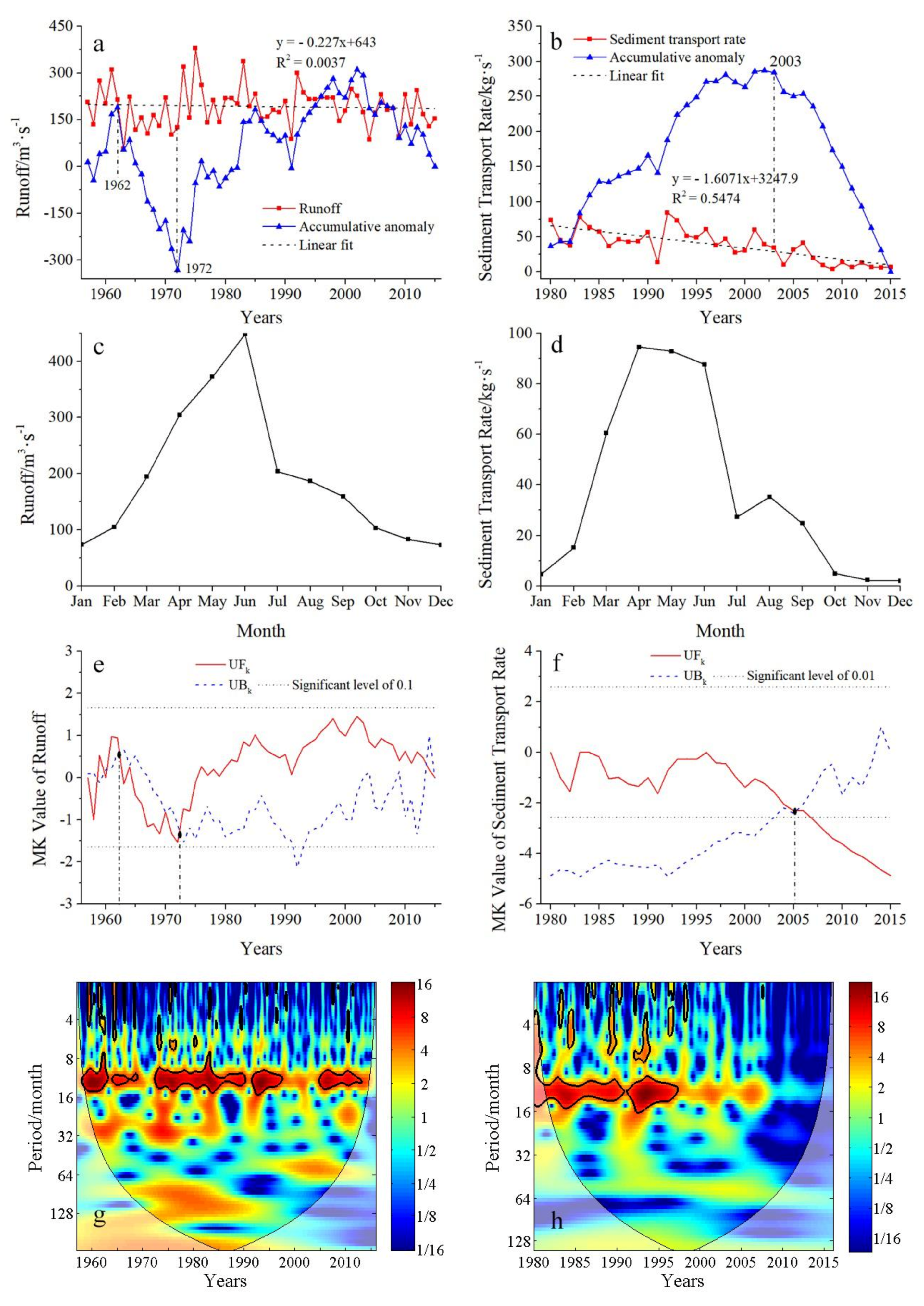
4.1.1. Inter-Annual Variation

The annual average runoff volume (Figure 2a) and the sediment transport rate (Figure 2b) showed overall declining trends, with the decreasing trend for the runoff volume being less obvious. The accumulative anomaly curve for the runoff (Figure 2a) changed in 1962 and 1972. In 1962, it changed from an increasing trend to decreasing, then returned to increasing in 1972. The declining trend for sediment transport was more obvious and occurred to a larger extent. The accumulative anomaly curve for the sediment transport rate (Figure 2b) changed from an increase to a decrease in 2003. The sediment transport rate reached its minimum values in 1991 and 2004, and the runoff volume during the same periods also reached its minimum values. This means that the runoff showed influences on sediment transport. From 2006 to 2015, the sediment transport volume (Figure 2b) decreased significantly, while such a decrease did not occur in the contemporaneous runoff volume (Figure 2a). The M-K trend analyses for the runoff and sediment transport showed that the annual average sediment transport rate passed the 0.01 significant level of the declining trend test, indicating that the decrease in the annual average sediment transport was significant. The annual average runoff, however, did not pass the significant change trend test, indicating that its changes were not significant within the time period.

4.1.2. Annual Variation

In the first half of a year, the runoff volume kept increasing and reached its maximum in June, then it kept decreasing in the second half of a year (Figure 2c). Generally, the runoff volume was relatively higher from March to June (the flood season). Compared with the annual runoff change, the sediment transport rate annual change had a similar pattern but with a shifted peaking time (Figure 2c,d). The sediment transport rate from March to June was much higher than that in other months (Figure 2d). It reached its peak value of 94.50 kg/s in April and decreased progressively in May and June, at 92.83 kg/s and 87.58 kg/s, respectively.

4.1.3. Mutation Analysis

The runoff volume UFk curve intersects the UBk curve in the years 1962 and 1972 (Figure 2e,f), which was consistent with the years showing accumulative anomaly variations. However, the UFk statistics did not exceed the critical value of the significance level of α = 0.1. Therefore, the changes of the runoff volume between 1957 and 2015 were insignificant.
The annual sediment transport rate mutation test showed that the UFk statistical value was positive only in the year 1996, but showed negative values in other years (Figure 2f), indicating that the descending trend for the sediment transport rate was dominant for the entire time sequence. In 2007, the statistical value for the sediment transport rate UFk exceeded the critical value of the significance level of α = 0.1, and a higher decreasing rate was observed. The forward and reverse M-K statistical values UFk and UBk intersect between 2005 and 2006. However, this intersection point is within the critical value of the significance level; thus, it could be concluded that the year 2005 was the mutation year of the sediment transport rate. In addition, the accumulative anomaly of the sediment transport volume began to decline in year 2003 and turned to a linear decreasing trend after 2005, which was consistent with the fact that the year 2005 was the starting time for the mutation. In fact, nine water conservancy projects were completed on the Taojiang River by the year 2005, and construction of the dams induced the decrease in sediment transport.

4.1.4. Periodic Variation

The fine lines in Figure 2g,h respectively represent the cone of influence (COI) and the energy spectrum beyond the curves, which shall be ignored due to the impact exerted by the boundary effects. The thick lines in the figures represent the critical value passing the 95% confidence level significance test [30]. The monthly runoff volume and sediment transport volume from 1957 to 2015 had different scales in the time-frequency domain and passed the 0.05 confidence level test. From 1958 to 1963, 1973 to 1990, 1991 to 1997, and 2004 to 2013, the runoff volume cycles in the low-energy region of the time-frequency domain lasted for 10 to 15 months (Figure 2g). For 1981–1990 and 1991–1997, the sediment transport volume cycles lasted for 10–16 months (Figure 2h).

4.2. Driving Factors of Runoff and Sediment Transport

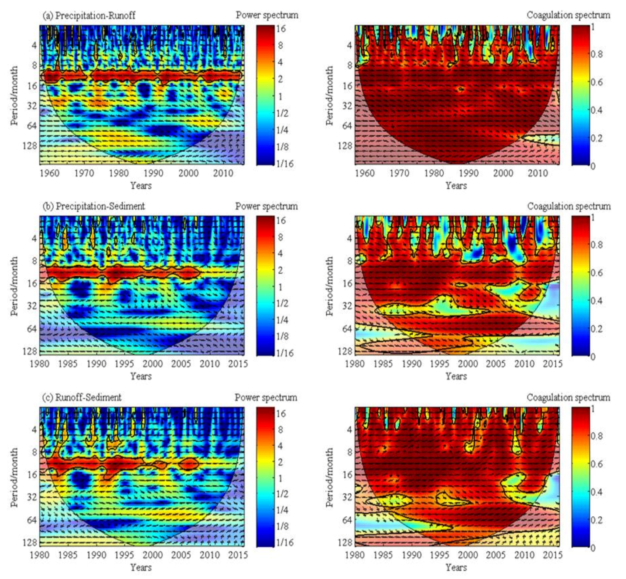
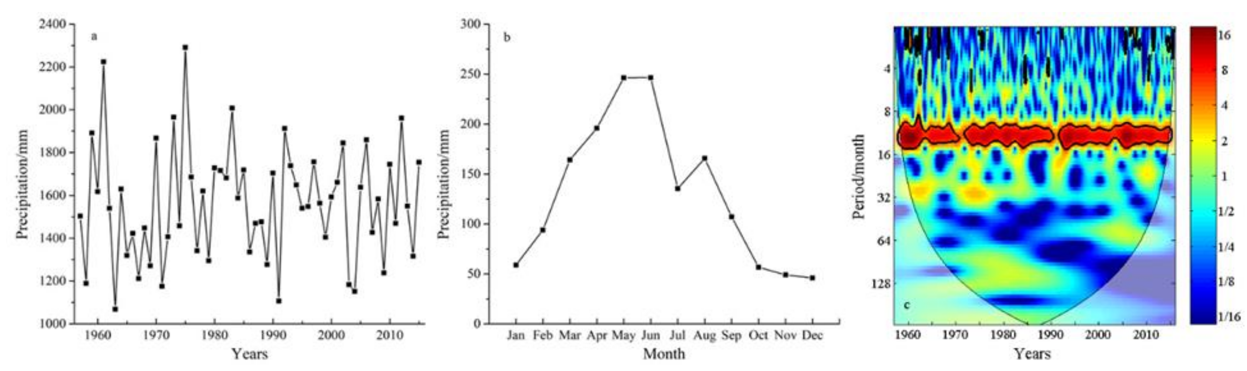
4.2.1. Precipitation

The annual precipitation from 1957 to 2015 is shown in Figure 3. The precipitation values were 2223.8 mm and 2291.4 mm in 1961 and 1975, respectively (Figure 3a) Despite the fluctuations from 1957 to 2015, there were no remarkable increase or decrease trends. Linear fitting was applied to the trend of annual average precipitation change, but it did not pass the significant correlation test.
From the annual precipitation distribution, it can be seen that the wet season was from March to August; the dry season was from October to the next January; and the normal season was in February and September (Figure 3b). The precipitation values in the wet, dry, and normal seasons accounted for 73.7%, 12.8%, and 13.5% of the total annual precipitation, respectively.
The continuous wavelet transform analysis of monthly precipitation from 1957 to 2015 (Figure 3c) showed that a significant cycle existed in the time-frequency domain, which passed the 0.05 confidence level test. The corresponding change cycle was about 1a, with interruptions occurring in 1971 and 1991.

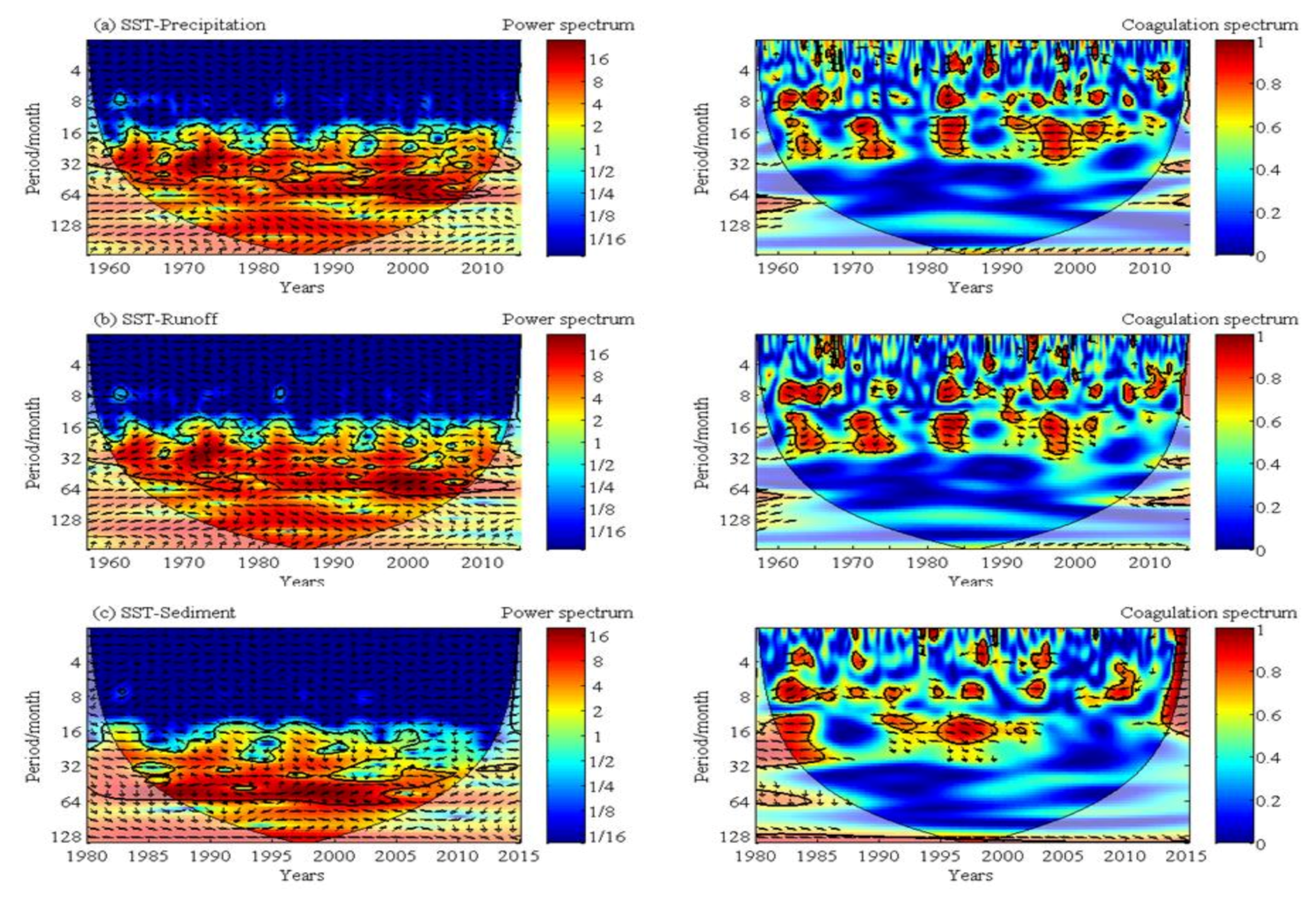
Cross-Wavelet Analysis of Precipitation, Runoff, and Sediment Transport

Figure 4a shows the results of cross-wavelet analyses applied to the monthly precipitation, runoff, and sediment transport volumes. In the cross-wavelet energy spectrum and coagulation spectrum of the precipitation and runoff volume, a significant resonance cycle with a magnitude of about 1 year was observed in the high-energy area, with one interruption occurring in 1971. During this period, the precipitation was positively correlated with the runoff volume and the correlation coefficient exceeded 0.9, proving that the precipitation was a dominant factor controlling the runoff volume. In the low-energy area, the significant resonance cycle area covered more than 90% of the entire wavelet coherence COI, which was consistent with previous studies [31,32,33].
Figure 4b shows the energy spectrum and coagulation spectrum related to the cross-wavelet analyses of precipitation and sediment transport volume. The variation cycle in the high-energy area was around 1a from 1980 to 2007, while the variation tendency within the cycle was similar to that in the precipitation–runoff cross-wavelet energy spectrum. From 2008 to 2015, there was no significant variation cycle between the precipitation and the sediment transport volume. After 2005, the significant resonance cycle in the low-energy area decreased remarkably.
Figure 4c shows the energy spectrum and coagulation spectrum related to the cross-wavelet analyses of runoff and sediment transport volume. The variation cycle of the high-energy area was around 1a from 1980 to 2001 and from 2005 to 2007, while the cycle variation tendency was similar to that of the precipitation–runoff and precipitation–sediment transport cross-wavelet energy spectra. From 2008 to 2015, no significant variation cycle was observed between the runoff and the sediment transport volume. Since 2006, the significant resonance cycle in the low-energy area has had a larger reduction than precipitation–sediment transport.
Figure 4 reveals that the differences in the phases among precipitation–runoff, precipitation–sediment, and runoff–sediment were identical in various time-frequency domains. However, the correlation between the runoff–sediment time-frequency domain changed and the precipitation–runoff time-frequency domains declined, while the precipitation–sediment time-frequency domain continued falling based on the runoff–sediment time-frequency domain, indicating that the runoff was the mediator between the precipitation and the sediment. Namely, the precipitation directly influenced the runoff and indirectly influenced the sediment transport by means of the runoff. Around 2005, a significant decline was observed from the significant resonance cycle area of the precipitation–sediment and runoff–sediment in the low-energy area occupied in the entire wavelet coherence COI, corresponding to the construction and operation time of a large-scale hydro-power station (Julongtan hydro-power station). Therefore, the hydro-power station played a significant role in reducing sediment transport induced by runoff.

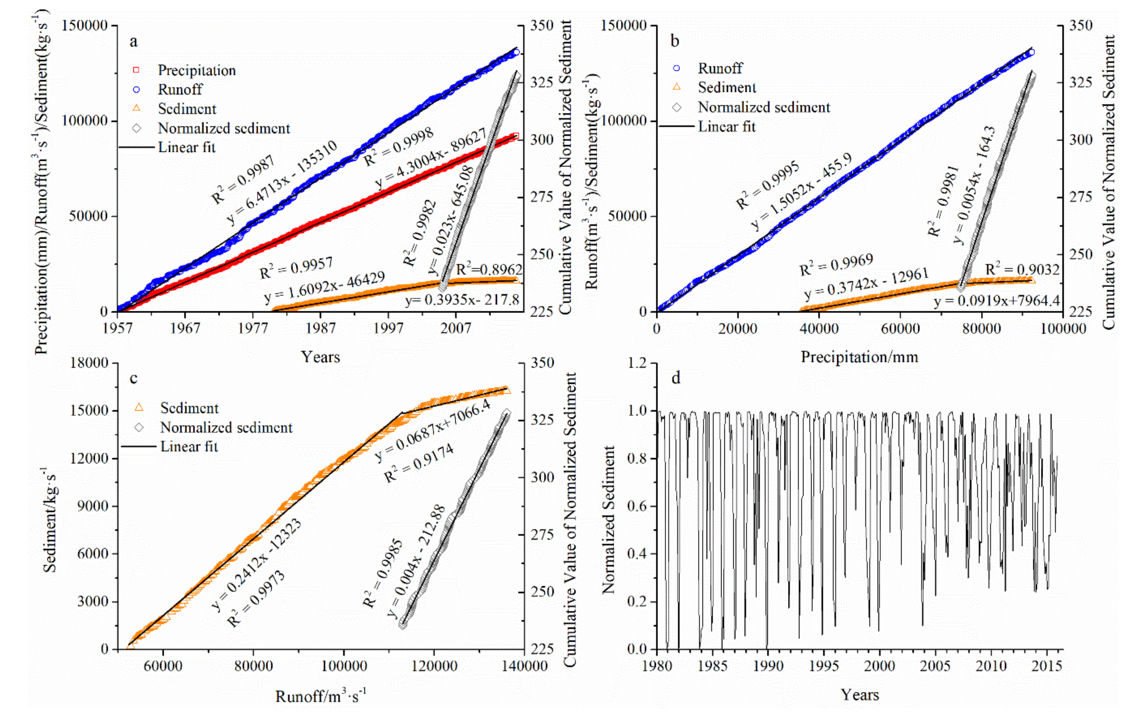
Quantitative Analysis of the Influence of Precipitation on Runoff and Sediment Transport

From the single accumulative figure (Figure 5a) showing the time sequences of the monthly precipitation and runoff volume from 1957 to 2015, it can be seen that the precipitation and runoff volume accumulative values were linearly correlated with time, with linear fitting R2 values of 0.9998 and 0.9987 for precipitation and runoff volume, respectively, indicating that the precipitation and runoff volume varied linearly with time, although the variation ranges were not significant.
The single accumulative curve (Figure 5a) for the time sequence of the monthly sediment transport rate from 1980 to 2015 revealed that a mutation occurred in the sediment transport rate in 2005, and that the sediment transport rate could be divided into two phases. In the first phase (from 1980 to 2004), the linear fitting R2 was 0.9957; in the second phase (from 2005 to 2015), the linear fitting R2 was 0.8962. The linear fitting curve slope in the second phase was obviously less than that in the first phase. Namely, the accumulative value of the annual sediment transport rate began to decline from the year 2005.
In general, the relationship between the double accumulative curve between precipitation, water, and sediment should be stable under natural conditions. When the curve turns, it represents a change occurring in the environment, which is often induced by human activities, such as construction of reservoirs and dams, which affect the water flow or sediment transport.
In the double mass accumulative curve (Figure 5b) for the time sequence of the annual precipitation and runoff volume from 1957 to 2015, the accumulative values for the runoff volume and precipitation were linearly correlated, with the linear fitting R2 at 0.9995, indicating that no significant increase or decrease was found in the precipitation yield within the basin.
In the double mass curve for annual precipitation and sediment transport volume in time sequence ranging from 1980 to 2015 (Figure 5b), a mutation occurred in 2005, which is consistent with the results of the M-K analysis for sediment transport. This curve could also be divided into two periods. In the first period (from 1980 to 2004), the linear fitting curve R2 was 0.9969; in the second period (from 2005 to 2015), the linear fitting curve R2 was 0.9032. The results of the hydrological estimation (Table 2) showed that the annual sediment transport volume in the second period decreased by 8.44 × 10⁷ t on average compared to the first period due to human activities, accounting for 95.7% of the total annual average sediment transport volume decrease. However, the decrease in sediment transport volume caused by the precipitation was 3.82 × 10⁶ t, only accounting for 4.3% of the total annual decrease. The ratio of influence of human activities and precipitation on the sediment transport volume was about 0.95:0.05.
A similar trend can be seen from the double mass curve (Figure 5c) of the time sequence of the annual runoff volume and sediment transport volume from 1980 to 2015. A mutation occurred in 2005. From 1980 to 2004, the linear fitting curve R2 was 0.9973; from 2005 to 2015, the linear fitting curve R2 was 0.9174. The fitting curve slope was smaller from 2005 to 2015 than that from 1980 to 2004. Based on the linear relationship between the runoff volume and sediment transport volume, the decrease in the sediment transport volume caused by the decline in the annual average runoff volume was 6.82 × 10⁷ t from 2005 to 2015.
In Figure 5a, a periodic sharp rise occurred in the year 2005 for the single accumulative value of the time sequence of the sediment transport volume. The same situation was observed for the double mass curves of the precipitation and sediment transport rate (Figure 5b) and for the runoff volume and sediment transport rate (Figure 5c). Therefore, the goodness of linear fitting was not very high. In combination with the actually measured data related to the sediment transport rate, the maximal sediment transport values occurred in June 2005 (167 kg/s), July 2006 (140 kg/s), June 2007 (163 kg/s), June 2008 (66.6 kg/s), June 2010 (79.9 kg/s), May 2011 (57.2 kg/s), March 2012 (48.6 kg/s), May 2013 (50.8 kg/s), May 2014 (52.5 kg/s), and May 2015 (52.6 kg/s). The monthly average sediment transport rate after taking out these maximal values was 4.66 kg/s. These maximal values were tens of times greater than the normal values (4.66 kg/s). Therefore, periodic sharp increases were observed from the accumulative value, which caused the same changes in the double mass curves of the precipitation, sediment transport rate, runoff volume, and sediment transport rate.
The normalization processing was performed for the sediment transport rate to eliminate the influence of the extremums. It was required to produce a single accumulative figure for the time sequence and double mass curve of precipitation and runoff volume (Figure 5d).

4.2.2. Water Conservancy Projects
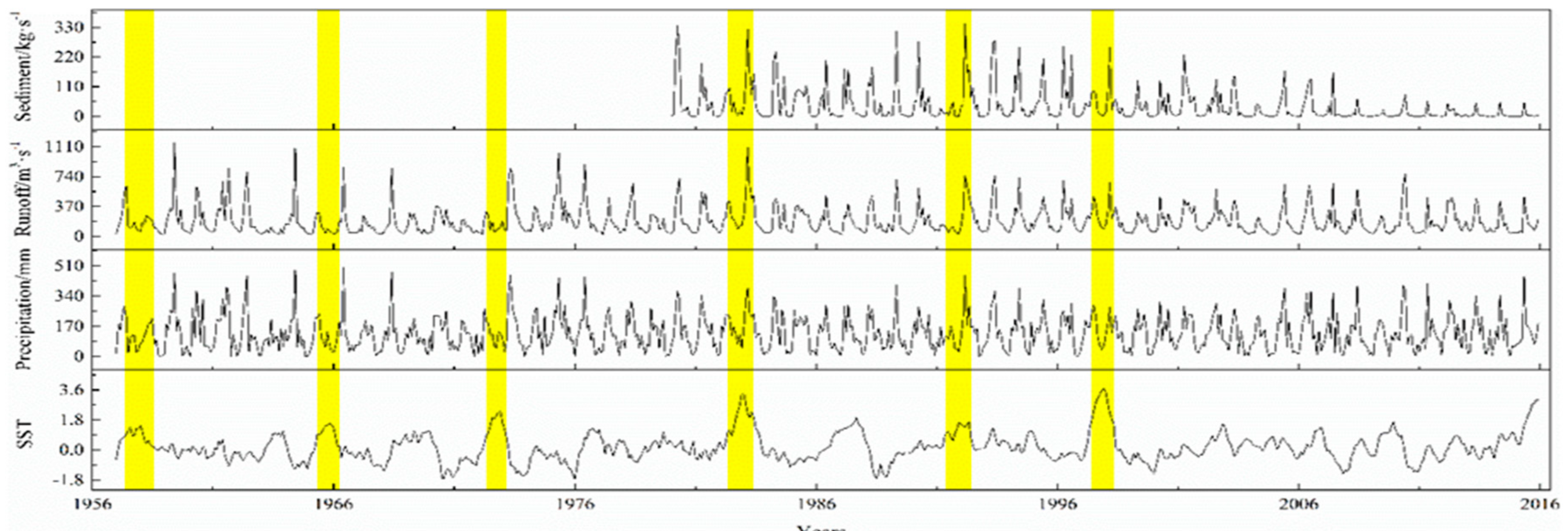
Among various human activities, soil and water conservation measures and the building of water conservancy structures are the main factors causing changes in the riverway runoff and sediment transport rate [34,35]. The following is a discussion on the influence of the building of water conservancy projects on the runoff and sediment transport in the study area.
The main features and parameters of these water conservancy projects are summarized in Table 3. The main water conservancy projects influencing the runoff volume and sediment transport volume from 1980 to 2015 included Longtoutan hydro-power station (built in 2000), Julongtan hydro-power station (built in 2004), and Taojiang hydro-power station (built in 2007). As Longtoutan hydro-power station was relatively small in capacity (1.38 × 10⁷ m3), it had an insignificant impact on the runoff volume and sediment transport volume. The capacities of Julongtan and Taojiang hydro-power stations were relatively larger, with an area of influence of 7739 km2 (accounting for 91.7% of the study area). These stations significantly influenced the runoff volume and sediment transport volume. Comprehensively, the completion times for the hydro-power stations were consistent with the mutation time (2005) of the runoff volume and sediment transport volume.
Table 1 and Table 2 show that the runoff and sediment transport decrease rates were 4.49 × 10⁷ m3/a and 6.57 t/a, respectively, for the water reservoirs. By adopting the prospective method based on the trend, the runoff and sediment transport decrease rates caused by construction of Zoumalong, Bailan, Wudugang, Shangjing, Longjing, and Zhongdun reservoirs before 1980 were 4.73 × 10¹⁰ m3/a and 6.91 × 10⁷ t/a, respectively. It can be concluded that the specific capacity of each reservoir was positively correlated to its water and sediment retaining capacities.

4.2.3. ENSO

Figure 6 shows the cross-wavelet analysis power spectrum and wavelet coherence analysis coagulation spectrum between the SST and various water features. The significant resonance cycles of the SST and precipitation (Figure 6a) in the high-energy area were concentrated at 1.33–4.00a from 1957 to 1982 and 1.30–5.30a from 1983 to 2015. During these cycles, the phase relation between SST and precipitation was subject to irregular changes. However, the significant resonance cycles in the low-energy area were concentrated at 1.00–2.30a from 1970 to 1974, 1982 to 1984, and 1995 to 1999. During these cycles, their correlation coefficients were close to 0.9.
Figure 6b shows the cross-wavelet analysis energy spectrum and coagulation spectrum between the SST and runoff volume. The significant resonance cycles in the high-energy area were concentrated at 1.33–4.67a from 1960 to 1982, 1.33–5.33a from 1983 to 1995, and 1.33–6.67a from 1996 to 2012. During these cycles, the phase relation between the SST and runoff volume was subject to random changes. The significant resonance cycles in the low-energy area were concentrated at 1.00–2.50a from 1970 to 1974, 1981 to 1984, and 1995 to 1998. During these cycles, the correlation coefficients exceeded 0.8.
Figure 6c presents the cross-wavelet analysis energy spectrum and coagulation spectrum between SST and sediment transport volume. The significant resonance cycles in the high-energy area were concentrated at 1.33–5.33a from 1960 to 2004, while the phase relation between the SST and sediment transport volume was positive after 1995. The significant resonance cycles in the low-energy area were concentrated at 1.00–1.67a from 1995 to 1998. During these cycles, the correlation coefficient exceeded 0.9. In combination with their cross-wavelet analysis energy spectrum and coagulation spectrum, the correlation changed in 2005 and was then scarcely correlated.
Further comparisons were made between the SST and precipitation, runoff, and sediment transport volume during major ENSO events (lasting for more than 10 months) from 1957 to 2015 (Figure 7). The durations of major ENSO events during this period were from April 1957 to July 1958, May 1965 to April 1966, May 1972 to March 1973, April 1982 to June 1983, May 1991 to June 1992, and May 1997 to May 1998. During each ENSO event, the SST first rose to a maximum and then declined, exhibiting a convex changing curve. The precipitation revealed a similar changing trend during each ENSO event—at the beginning of each ENSO event, it declined to the minimum and then increased; at later stages, it reached its maximum and then declined again. During each ENSO event, the changing trend for runoff and sediment transport volume was basically similar to that of precipitation. ENSO influences the rainfall related to precipitation, which affect the runoff and consequently affect sediment transport.
Due to the global climate change in recent years, ENSO events occur frequently, which consequently induce natural hazards. The approaches used in this study, together with the findings obtained, may provide a scientific basis for decision makers, such as local governments, to make plans and take measures against natural hazards in advance or in the early stages of an abnormal event.

5. Conclusions

From the results of this study, the following conclusions can be drawn:
  • A mutation occurred in the sediment transport rate in 2005 and a significant decline was observed as well. However, no significant change was found in the runoff volume from 1957 to 2015. From the year 2005 onwards, the annual average decrease of sediment transport volume was 8.82 × 10⁷ tons;
  • The precipitation was the dominant factor that controlled the changes in runoff volume and sediment transport volume, since the precipitation directly influenced changes of the runoff volume, which subsequently caused changes in the sediment transport rate in the river basin. From the year 2005 onwards, changes in the sediment transport rate were heavily influenced by the large-scale hydro-power stations (Taojiang and Julongtan), with a significant declining trend observed. The annual sediment transport decreased by 8.44 × 10⁷ tons during 1980–2004 and 2005–2015, accounting for 95.7% of the total decrease in the sediment transport volume;
  • Significant resonance cycles between SST and the precipitation, runoff volume, and sediment transport mainly covered the 1.33–5.33a-year period. During the ENSO events, the precipitation, runoff volume, and sediment transport rate reached their maximums after a decline at the beginning of each event, and then eventually decreased again.
Although this study analyzed various drivers of runoff and sediment transport variations in the Taojiang River drainage basin with distributed ion-type RE mine lots, no scientific studies were conducted on the impacts of the RE mining activities on soil erosion or the subsequent influences on the runoff and sediment transport in this river basin. This missing information will be the priority of the follow-on research effort in this project.

Author Contributions

Conceptualization, Y.L (Youcun Liu) and M.C.; methodology, Y.L. (Youcun Liu) and Q.D.; software, Y.M.; validation, M.C., D.L. and M.Z.; formal analysis, Y.L. (Youcun Liu) and Q.D.; investigation, Y.L. (Youcun Liu); resources, M.C. and Y.L. (Yongtao Li); data curation, Y.L. (Youcun Liu); writing—original draft preparation, Y.L. (Youcun Liu) and Q.D.; writing—review and editing, L.Z. and D.L.; visualization, Q.D.; supervision, M.Z. and M.C.; project administration, M.C.; funding acquisition, Y.L. (Youcun Liu) and Y.L. (Yongtao Li). All authors have read and agreed to the published version of the manuscript

Funding

This research was funded by the National Natural Science Foundation of China (grant number 41861002 & 51664025), the Natural Science Foundation of Jiangxi Province (grant number 20181BAB203026), and the Innovative Talent Project of Ganzhou City Science Foundation (grant number Gankefa2019[60]).

Acknowledgments

We would like to express our deepest gratitude to the anonymous reviewers for their constructive comments and very helpful suggestions.

Conflicts of Interest

The authors declare no conflict of interest.

References

  1. Lal, R. Soil degradation by erosion. Land Degrad. Dev. 2001, 12, 519–539. [Google Scholar] [CrossRef]
  2. Morgan, R.P.C. Soil Erosion and Conservation, 3rd ed.; Blackwell Publishing: Oxford, UK, 2009. [Google Scholar]
  3. Cerdan, O.; Govers, G.; Le Bissonnais, Y.; Van Oost, K.; Poesen, J.; Saby, N.; Gobin, A.; Vacca, A.; Quinton, K.; Auerswald, K.; et al. Rates and spatial variations of soil erosion in Europe: A study based on erosion plot data. Geomorphology 2010, 122, 167–177. [Google Scholar] [CrossRef]
  4. Carroll, C.; Merton, L.; Burger, P. Impact of vegetative cover and slope on runoff, erosion, and water quality for field plots on a range of soil and spoil materials on central Queensland coal mines. Soil Res. 2000, 38, 313–328. [Google Scholar] [CrossRef]
  5. Wantzen, K.M.; Mol, J.H. Soil erosion from agriculture and mining: A threat to tropical stream ecosystems. Agriculture 2013, 3, 660–683. [Google Scholar] [CrossRef] [Green Version]
  6. Martín-Moreno, C.; Martín Duque, J.F.; Nicolau Ibarra, J.M.; Hernando Rodríguez, N.; Sanz Santos, M.Á.; Sánchez Castillo, L. Effects of topography and surface soil cover on erosion for mining reclamation: The experimental spoil heap at El Machorro Mine (Central Spain). Land Degrad. Dev. 2016, 27, 145–159. [Google Scholar] [CrossRef] [Green Version]
  7. Wang, P.; Liu, S.F. Status of soil erosion of south China rare-earth mining area. Soil Water Conserv. China 2008, 3, 44–46. [Google Scholar]
  8. Zheng, T.; Yang, J.; Huang, P.; Tang, C.; Wan, J. Comparison of trace element pollution, sequential extraction, and risk level in different depths of tailings with different accumulation age from a rare earth mine in Jiangxi Province, China. J. Soil Sediment 2018, 18, 992–1002. [Google Scholar] [CrossRef]
  9. Wen, X.J.; Zhang, D.C. Effect of resource exploitation on soil environment and rare earth bioavailable fractions in plough layer of mining area. China Min. Mag. 2012, 21, 44–47. [Google Scholar]
  10. Yang, X.J.; Lin, A.; Li, X.L.; Wu, Y.; Zhou, W.; Chen, Z. China’s ion-adsorption rare earth resources, mining consequences and preservation. Environ. Dev. 2013, 8, 131–136. [Google Scholar] [CrossRef]
  11. Li, Y.X.; Zhang, L.; Zhou, X.M. Resource and environment protected exploitation model for ion-type rare earth deposit in southern of China. Chin. Rare Earths 2010, 31, 80–85. [Google Scholar]
  12. Liu, Y.; Liu, Z.; Liu, J.; Chen, M.; Zhang, J.; Xu, Y.; Liu, M. Distribution characteristics and risk assessment of ammonia nitrogen and heavy metal pollution in longjing river, the upstream of ganjiang river. Nonferr. Met. Sci. Eng. 2019, 10, 85–93. [Google Scholar]
  13. Liao, Z.; He, W.; Liu, H.; Wang, X. Quality assessment of geological environment of ion-absorbed rare-earth mine in Longnan County. Nonferr. Met. Sci. Eng. 2014, 5, 106–111. [Google Scholar]
  14. Liu, S.W.; Liu, X.D.; Tan, K.Y.; Huang, Y.Y. Characteristics of soil pollution caused by mining in ion-absorbed rare earth mines and crucial issues of the polluted soil restoration: A case study of longnan rare earth mines, south china. Adv. Mater. Res. 2014, 955–959, 2564–2569. [Google Scholar] [CrossRef]
  15. Zou, G.; Wu, Y.; Cai, S. Impacts of ion-adsorption rare earth’s leaching process on resources and environment. Nonferr. Met. Sci. Eng. 2014, 5, 100–106. [Google Scholar]
  16. Sarachik, E.S.; Cane, M.A. The El Nino-southern Oscillation Phenomenon; Cambridge University Press: Cambridge, UK, 2010. [Google Scholar]
  17. Liu, Y.; Lu, M.; Huo, X.; Hao, Y.; Gao, H.; Cui, Y.; Metivier, F. A Bayesian analysis of generalized pareto distribution of runoff minima. Hydroll. Process. 2016, 30, 424–432. [Google Scholar] [CrossRef]
  18. Mann, H.B. Non-parametrictests against trend. Econometrica, 1945; 13, 163–171. [Google Scholar]
  19. Kendall, M.G. Rank Correlation Methods, 4th ed.; Charles Griffin: London, UK, 1975. [Google Scholar]
  20. Liu, Y.; Liu, Y.; Chen, M.; Labat, D.; Li, Y.; Bian, X.; Ding, Q. Characteristics and drivers of reference evapotranspiration in hilly regions in southern China. Water 2019, 11, 1914. [Google Scholar] [CrossRef] [Green Version]
  21. Wang, F.; Shao, W.; Yu, H.; Kan, G.; He, X.; Zhang, D.; Ren, M.; Wang, G. Re-evaluation of the power of the Mann-Kendall test for detecting monotonic trends in hydrometeorological time series. Front. Earth Sci. 2020. [Google Scholar] [CrossRef]
  22. Grinsted, A.; Moore, J.C.; Jevrejeva, S. Application of the cross wavelet transform and wavelet coherence to geophysical time series. Nonlinear Proc. Geophys. 2004, 11, 561–566. [Google Scholar] [CrossRef]
  23. Ding, Q.; Liu, Y.; Jiao, K.; Bian, X.; Liu, Y. Changes and driving factors of runoff and sediment yield of typical watershed in upper reaches of Ganjiang River. Bull. Soil Water Conserv. 2018, 38, 19–26, 33. [Google Scholar]
  24. Zhao, Z.H. Study on Non-point Pollution in Tao River Basin’s Agricultural Field Based on AnnAGNPS Model. Jiangxi: Nanchang Univ. 2012. [Google Scholar] [CrossRef]
  25. Yamasaki, K.; Gozolchiani, A.; Havlin, S. Climate networks around the globe are significantly affected by El Nino. Phys. Rev. Lett. 2008, 100, 228501. [Google Scholar] [CrossRef]
  26. Collins, M.; An, S.I.; Cai, W.; Ganachaud, A.; Guilyardi, E.; Jin, F.F. The impact of global warming on the tropical Pacific Ocean and El Niño. Nat. Geosci. 2010, 3, 391–397. [Google Scholar] [CrossRef]
  27. Adamowski, J.F. River flow forecasting using wavelet and cross-wavelet transform models. Hydrol. Process. An Int. J. 2008, 22, 4877–4891. [Google Scholar] [CrossRef]
  28. Labat, D. Cross wavelet analyses of annual continental freshwater discharge and selected climate indices. J. Hydrol. 2010, 385, 269–278. [Google Scholar] [CrossRef]
  29. Labat, D.; Ababou, R.; Mangin, A. Wavelet analysis in karstic hydrology. 2nd part: Rainfall-runoff cross-wavelet analysis. Comptes rendus de l’Academie des Sciences. Serie 2. Fascicule a. Sciences de la terre et des planetes/Earth and planetary sciences. Montrouge 1999, 329, 881–887. [Google Scholar]
  30. Yu, H.L.; Lin, Y.C. Analysis of space–time non-stationary patterns of rainfall–groundwater interactions by integrating empirical orthogonal function and cross wavelet transform methods. J. Hydrol. 2015, 525, 585–597. [Google Scholar] [CrossRef]
  31. Fekete, B.M.; Vörösmarty, C.J.; Roads, J.O.; Willmott, C.J. Uncertainties in precipitation and their impacts on runoff estimates. J. Climate 2004, 17, 294–304. [Google Scholar] [CrossRef]
  32. Xu, K.; Milliman, J.D.; Xu, H. Temporal trend of precipitation and runoff in major Chinese rivers since 1951. Glob. Planet Chang. 2010, 73, 219–232. [Google Scholar] [CrossRef]
  33. Liu, Y.; Wu, J.; Liu, Y.; Hu, B.X.; Hao, Y.; Yeh, T.J.; Wang, Z.L. Analyzing effects of climate change on streamflow in a glacier mountain catchment using an ARMA model. Quatern. Int. 2015, 358, 137–145. [Google Scholar] [CrossRef]
  34. Ren, L.; Wang, M.; Li, C.; Zhang, W. Impacts of human activity on river runoff in the northern area of China. J. Hydrol. 2002, 261, 204–217. [Google Scholar] [CrossRef]
  35. Liu, Y.; Métivier, F.; Gaillardet, J.; Ye, B.; Meunier, P.; Narteau, C.; Lajeunesse, E.; Han, T.; Malverti, L. Erosion rates deduced from seasonal mass balance along the upper Urumqi River in Tianshan. Solid Earth 2011, 2, 283–301. [Google Scholar] [CrossRef] [Green Version]
Figure 1. Sketch map of the study area.
Water 12 02283 g001
Figure 2. Variations of runoff (a) for 1957–2015 and sediment transport rate (b) for 1980–2015 on inter-annual scales. Variations of runoff (c) and sediment transport rate (d) on annual scales (averaged over the measurement periods). Mann–Kendall (M-K) inspection (e,f) and continuous wavelet (g,h) analysis of the data collected at Julongtan station over the measurement periods.
Water 12 02283 g002
Figure 3. The inter-annual (a) and annual (b) changes of precipitation and the continuous wavelet transform analysis (c).
Water 12 02283 g003
Figure 4. The cross-wavelet analysis of precipitation and runoff(a), precipitation and sediment transport(b), runoff and sediment transport (c).
Water 12 02283 g004
Figure 5. Accumulative curves (a) for 1957–2015 and double mass curves (b,c) for precipitation, runoff, and sediment transport in the study area, along with normalized sediment (d) for 1980–2015 over the measurement periods.
Water 12 02283 g005
Figure 6. Cross-wavelet analysis between the SST and precipitation (a), runoff (b), and sediment transport (c) volume.
Water 12 02283 g006
Figure 7. Changes of the SST and precipitation, runoff, and sediment transport volume in the study area during major ENSO events.
Water 12 02283 g007
Table 1. Measurement stations located in the study area.
Data TypeStationLongitudeLatitudeTime Period
RunoffJulongtan115°07′ E25°49′ N1957–2015
SedimentJulongtan115°07′ E25°49′ N1980–2015
SST 160°W–90° W5°N–5° S1957–2015
PrecipitationShanggankeng114°19′ E24°43′ N1980–2015
Gupi115°06′ E25°20′ N1965–2015
Jinpenshan115°12′ E25°16′ N1962–2015
Xintian115°15′ E25°22′ N1965–2015
Pitou114°35′ E25°01′ N1977–2015
Longyuanba114°27′ E24°56′ N1964–2015
Yuezi115°18′ E24°40′ N1963–2015
Luokeng114°19′ E24°37′ N1984–2015
Makenggang114°24′ E24°37′ N1980–2015
Dutou114°38′ E24°47′ N1958–2015
Guankeng114°40′ E24°39′ N1981–2015
Henggang114°42′ E24°36′ N1977–2015
Jiahu114°39′ E24°44′ N1964–2015
Shangwei114°30′ E24°35′ N1980–2015
Shuangluo114°36′ E24°43′ N1980–2015
Yangcun114°38′ E24°39′ N1980–2015
Chayuan114°58′ E25°24′ N2001–2015
Dajishan114°22′ E24°37′ N1962–2015
Hengxi115°01′ E25°35′ N1962–2015
Huangpodi115°12′ E25°38′ N1965–2015
Julongtan115°07′ E25°49′ N1957–2015
Nanjing114°23′ E24°41′ N1977–2015
Xinfeng114°56′ E25°23′ N1957–2015
Yangfang114°14′ E24°41′ N1980–2015
Zhushanxia114°18′ E24°40′ N1980–2015
Wenlong114°54′ E24°46′ N1963–2015
Youshan114°42′ E25°25′ N1962–2015
Table 2. Decrease in sediment transport in the study area.
Years Decrease in the Sediment Transport/(104 t/year)Decrease in the Sediment Transport Caused by the Runoff Volume (104 t/year)
Human ActivitiesTotal Decrease
2005–20158440.798822.376817.99
Table 3. Water conservancy projects on the Taojiang River.
Water Conservancy ProjectRiver SystemDrainageArea/km2Total Storage Capacity/104 m3Year of CompletionReinforcement Time
Zoumalong reservoirXihe River91.62 3701958
Bailan reservoirAnxi River24.41 16019601998–2000
Wudugang reservoirXiaohe River1203 33019612004/05–2005/07
Shangjing reservoirAnxi River31.61 1851967
Longjing reservoirDonghe River1401 3851969
Zhongcun reservoirXihe River29.21 0921976
Longtoutan hydro-power stationTaojiang River2 6531 3802000
Taojiang hydro-power stationTaojiang River3 6793 7102004
Julongtan hydro-power stationTaojiang River7 7397 7602007

