Global River Monitoring Using Semantic Fusion Networks

Abstract

Global river monitoring is an important mission within the remote sensing society. One of the main challenges faced by this mission is generating an accurate water mask from remote sensing images (RSI) of rivers (RSIR), especially on a global scale with various river features. Aiming at better water area classification using semantic information, this paper presents a segmentation method for global river monitoring based on semantic clustering and semantic fusion. Firstly, an encoder–decoder network (AEN)-based architecture is proposed to obtain the semantic features from RSIR. Secondly, a clustering-based semantic fusion method is proposed to divide semantic features of RSIR into groups and train convolutional neural networks (CNN) models corresponding to each group using data augmentation and semi-supervised learning. Thirdly, a semantic distance-based segmentation fusion method is proposed for fusing the CNN models result into final segmentation mask. We built a global river dataset that contains multiple river segments from each continent of the world based on Sentinel-2 satellite imagery. The result shows that the F1-score of the proposed segmentation method is 93.32%, which outperforms several state-of-the-art algorithms, and demonstrates that grouping semantic information helps better segment the RSIR in global scale.

1. Introduction

Rivers play an important role in both nature and the human civilization system, as they connect surface water bodies and deliver fresh water to ecosystems and societies in different districts [1,2]. Monitoring rivers globally can help us identify extreme river events and climate change, such as flooding and drought, that have a lot of implications for human–nature relationships [3,4,5,6,7].

With the recent development of satellite technologies, remote sensing data have become available for large-scale monitoring [8]. However, obtaining accurate global knowledge of the spatiotemporal dynamics of rivers still remains challenging for several reasons [9,10]. Firstly, in situ gauge river data is rarely available, and it is also sparsely distributed over different regions around the world. This requires the development of new methods in order to learn efficiently from limited labeled data [11]. Secondly, traditional methods such as threshold classification cannot precisely map a river’s extent due to its variability over time [12]. For example, Figure 1 shows a series of remote sensing images of a typical river (an actual river located in the northern part of the Republic of Colombia) within a year. We can easily observe its typical characteristics, whereby the river and its surrounding land cover show different reflectance spectral features over time. The image visualization was generated using Sentinel-2 imagery, in a false color composite style with Band #9 (Band name: Water vapour), #7 (Band name: Vegetation Red Edge) and #3 (Band name: Green) (the false color images shown in the rest of this paper follow same fashion), which is one of the common visualization methods for multi-spectral data. The challenges to water mapping caused by variability become even more serious when we monitor rivers on a global scale, since the spectral features of rivers can vary both across different regions and across different time periods [13].

Many existing studies on river mapping use two-band water indices [14]. The idea is to enhance the water representation based on the reflectance characteristics of water. Several index methods have been proposed, such as normalized difference water index (NDWI) [15] and its variant, modified normalized difference water index (MNDWI) [16]. The index values are thresholded to differentiate between water and land. The reflectance characteristics are dependent on water quality, which varies across different regions, and thus the threshold is highly dependent on the specific study region under consideration [17]. Moreover, the use of a water index results in similar representations for water, shadow and snow [18], making large-scale monitoring even more challenging.

Pixel-based machine learning algorithms [19], such as Support Vector Machine (SVM) [20,21,22], Decision Trees [23], Random Forest [24,25] and Quantile Regression Forests (QRF) [26,27] have also commonly been used to detect rivers. Compared with the water index, machine learning methods are better able to represent water characteristics by leveraging multiple bands available for the river in RSI [28]. However, pixel-based methods ignore the spatial relationship between pixels, and thus are highly likely to be impacted by noise in an RSI [29]. Additionally, image-level information, such as shape and compactness, is cannot be acquired to help with classification in pixel-based machine learning methods [30].

CNNs have been used in computer vision and remote sensing [31,32,33]. Compared to machine learning methods, the concept of the receptive field has significantly improved the performance deep learning methods by capturing the space and time relationship between each individual pixel and its neighborhood [34]. The CNN-based method has also shown better performance for water mapping in selected regions [35,36].

Ideally, with sufficient training data for rivers distributed over different regions and different periods, a single deep learning model can be built for water detection at a global scale [37,38]. However, in practice, the data is only available at specific water sites, leading to low performance on an unseen water region [39]. One possible solution could be to let the segmentation process follow the model, using similar water regions to the unseen water region. This idea attempts to enhance a specific type of water’s representation during water/land segmentation.

The algorithm in this paper first proposes a transform and clustering method to capture the semantic relationship of the RSIR. Starting from a set of labeled and unlabeled RSIR, a simple encoder–decoder network (AEN) is proposed to capture the representative information of each RSIR, by transforming the RSIR from a multi-band feature to single band feature (SBF) using AEN. Then, in order to capture the semantic relationship between SBF, the flattened SBF is a secondary dimension transformed using t-distributed stochastic neighbor embedding (TSNE) [40], and then the labeled RSIR are clustered into groups of RSIR by K-means [41].

To generate accurate water masks of RSIR, we propose a new learning framework for training deep learning models and fusing results from different groups of RSIR. Firstly, different CNN models are trained based on corresponding groups of RSIR clustered based on the semantic relationship of the RSIR. During this processing, we specifically address the few-shot issues within the RSIR group by proposing a semi-supervised learning method. That is, we first train an AEN model using unlabeled RSIR. Then we initialize the parameters of the segmentation model (the feature extraction part) using the estimated parameters from the AEN model. This method achieves faster training speed and greater robustness compared with other supervised training methods.

Finally, the unlabeled RSIR targets are segmented by all CNN models, and fused with all the segmentation into a final segmentation result. Here, a similarity-based fusion method is proposed to combine multi segmentation into single segmentation result. The idea is to segment the unlabeled RSIR combing the knowledge from both the nearest model in semantic space, and the surrounding semantic models.

In this paper, we propose an ensemble deep learning method for global water detection. Compared with common machine learning, and deep learning models, our method shows better performance in generating accurate water masks on a global scale.

The rest of this paper is organized as follows. Section 2 presents the proposed method. Section 3 reports the experiment results and discussion. Section 4 concludes this paper.

2. Materials and Methods

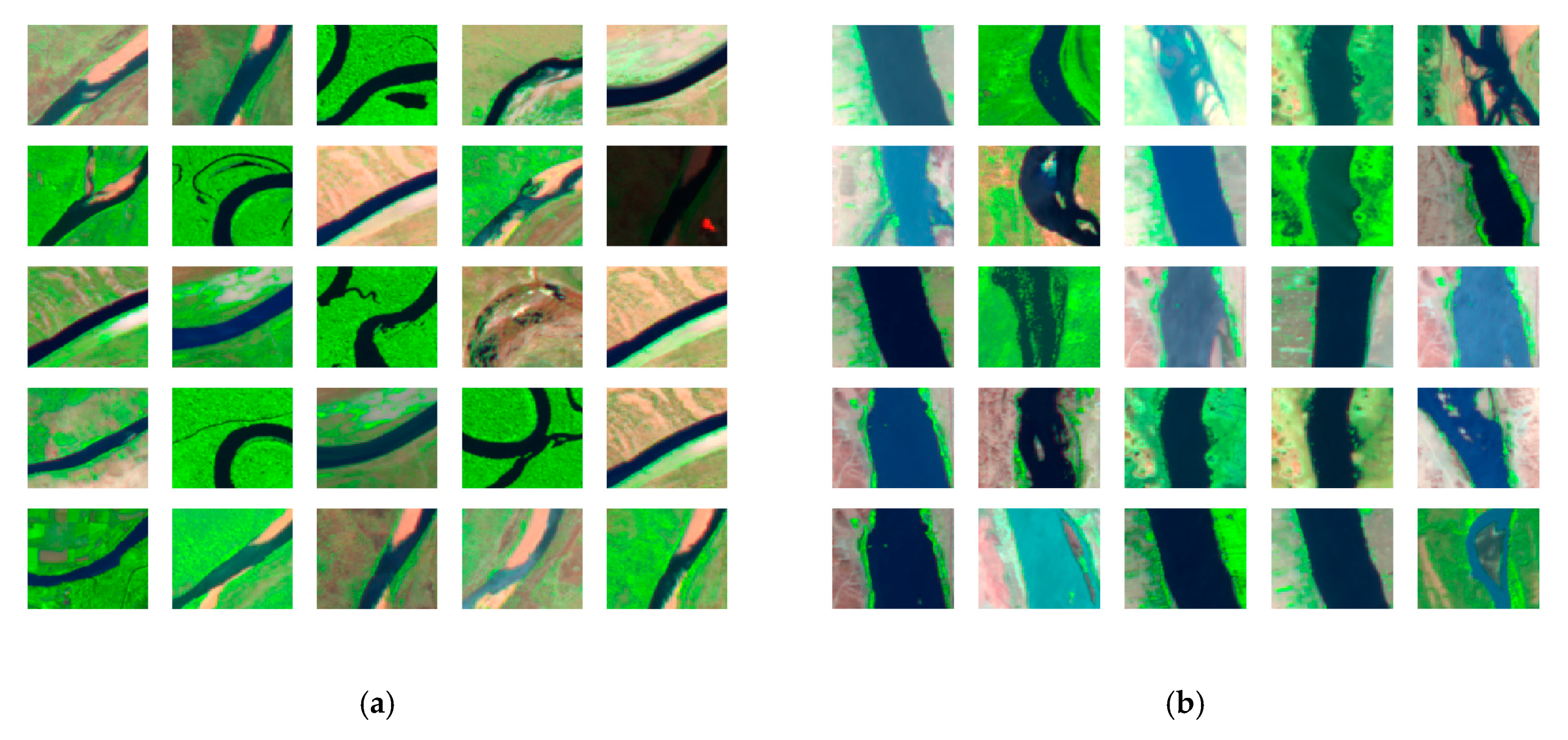
2.1. Study Area and Data

To collect river data globally, we first built a global RSIR dataset from the Sentinel-2 Imagery, and spent several months manually marking accurate water surface areas of river as ground truth within each river imagery. The Sentinel-2 Imagery contains accessible high-resolution remote sensing images that range from 10 m to 60 m; more detailed information is shown in

Table 1. Detailed information for Sentinel-2 satellite imagery.

Parameter Type		Detail
Sources		Sentinel-2
resolution	temporal	10 days
	spatial	10 m, 20 m, 60 m
spectral range		0.04–0.24 μm
orbital altitude		786 km

.

In total, the dataset we built contains about 15,000 river samples, along with 2700 manual ground truths.

As shown in Figure 2, the dataset includes different types of river from all continents. Specifically, the locations we selected in each continent were spread across very different climates, and belonged to different hydrological regions. We constructed the dataset by selecting locations from the Google Earth Engine, and acquired remote sensing images covering one square kilometer areas from the Sentinal-2 satellite collected in 2016.

Figure 3 shows a zoomed in detail from the black circle area in Figure 2, located in the Northern part of South America.

Figure 4 shows an example of the sample visualization and manual ground truth in the dataset. Each sample contains a 96 × 96 × 9 reflectance characteristics matrix and a 96 × 96 ground truth matrix, which represents a 1 km × 1 km area. The reflectance characteristics matrix contains nine sentinel-2 bands, with a resolution of 10 m and 20 m. These band ids are bands #2, #3, #4, #5, #7, #8, #8A, #11, #12.

To visualize the various types of river in the dataset, we applied the K-means method on the collected global river dataset and select two categories from various types of rivers, as shown in Figure 5.

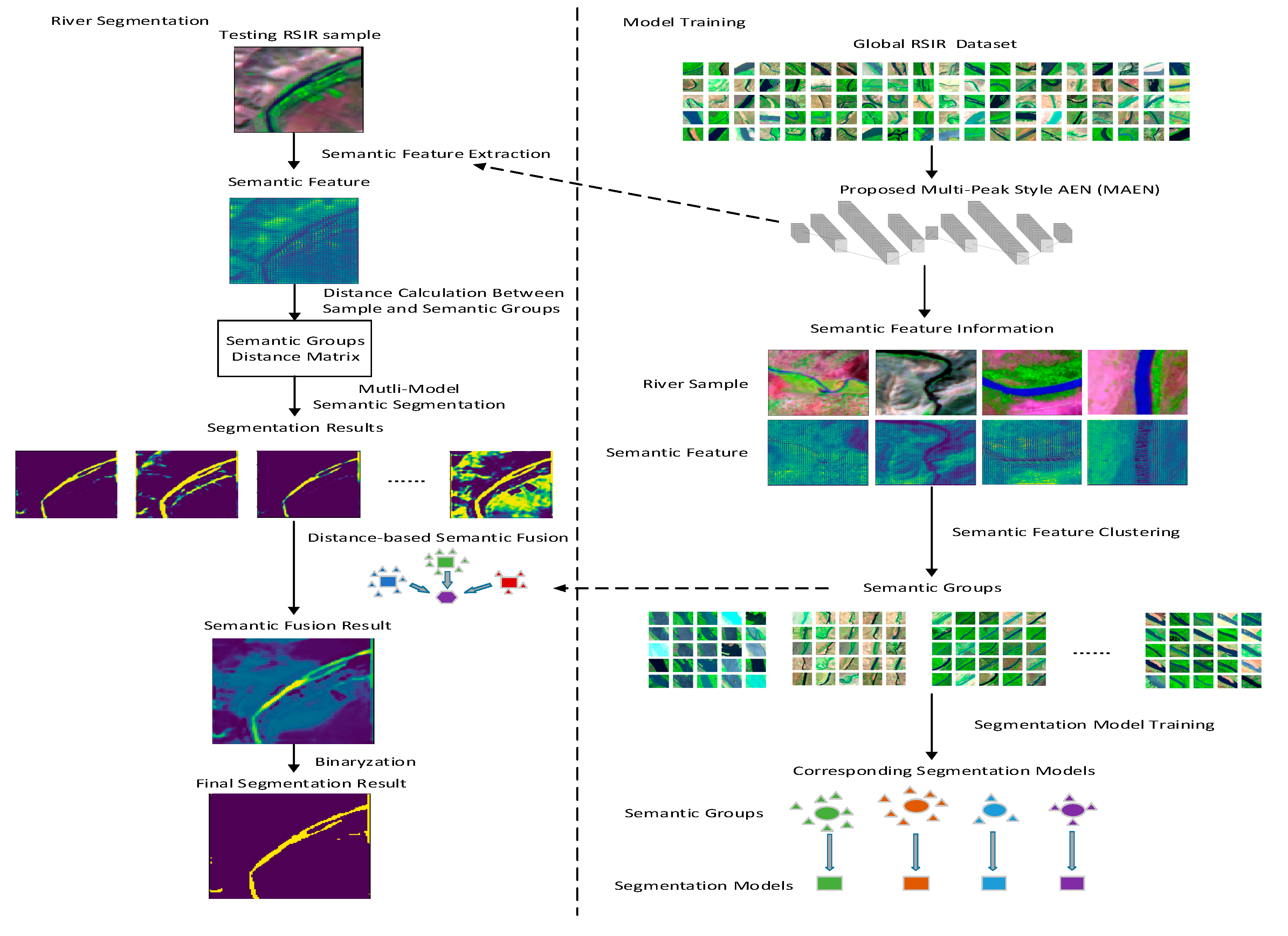
2.2. Proposed Method

In this section, we present the proposed methods for the global river segmentation task. Firstly, Figure 6 shows the proposed semantic fusion structure.

The definition of the input for the method is as follows: $X=(p_1,p_2,\dots ,p_i)$, which represents samples from the global RSIR dataset, including $X_a\in X$, which were labeled using a water mask, and $X_b\in X$, which were not labeled using a water mask. During the training process, the semantic features of the RSIR are extracted by a proposed multi-peak style AEN (MAEN) structure-based semantic feature extraction structure, and clustered into serval semantic groups. Then, serval segmentation models are trained based on the RSIR samples corresponding to the semantic features within each semantic groups. During the River segmentation process, the testing RSIR sample is first transformed into semantic feature through MAEN. Based on the proposed ensemble learning-based similarity fusion method, multi-segmentation results are fused into a single segmentation result based on the semantic distance between the testing RSIR samples and each semantic group.

The rest of this section is organized as follows. Firstly, we proposed an AEN-based semantic feature extraction structure. Secondly, we design a clustering process based on extracted semantic feature, and train the models based on the clustered samples from $X_a$. Furthermore, we present a semi-supervised learning based on information transform method to better initialized the CNN model. Finally, we propose similarity-based fusion method for global RSIR segmentation based on CNN.

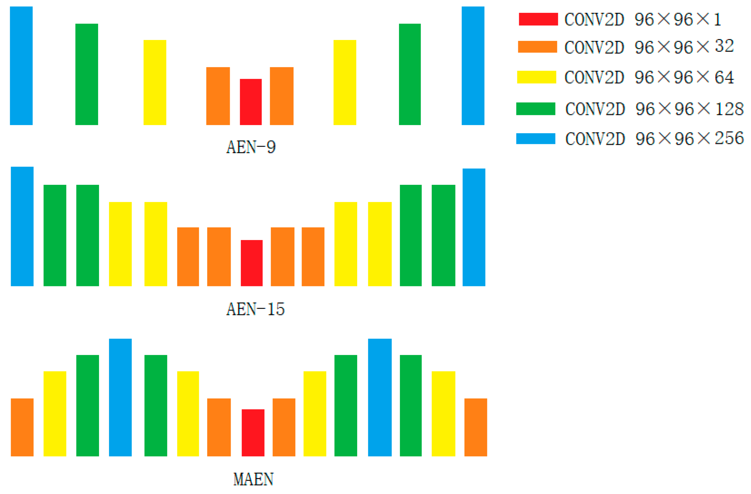
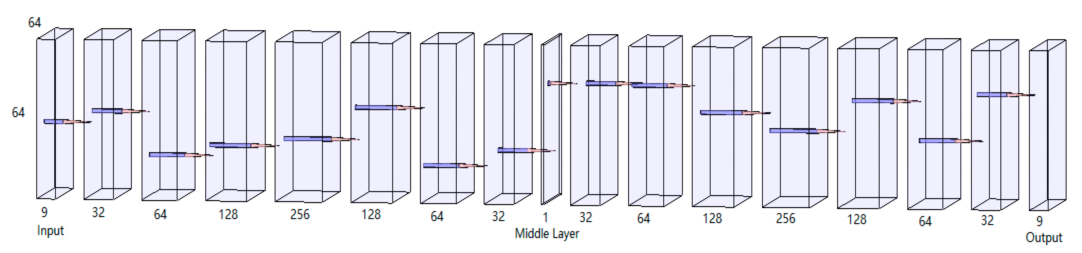
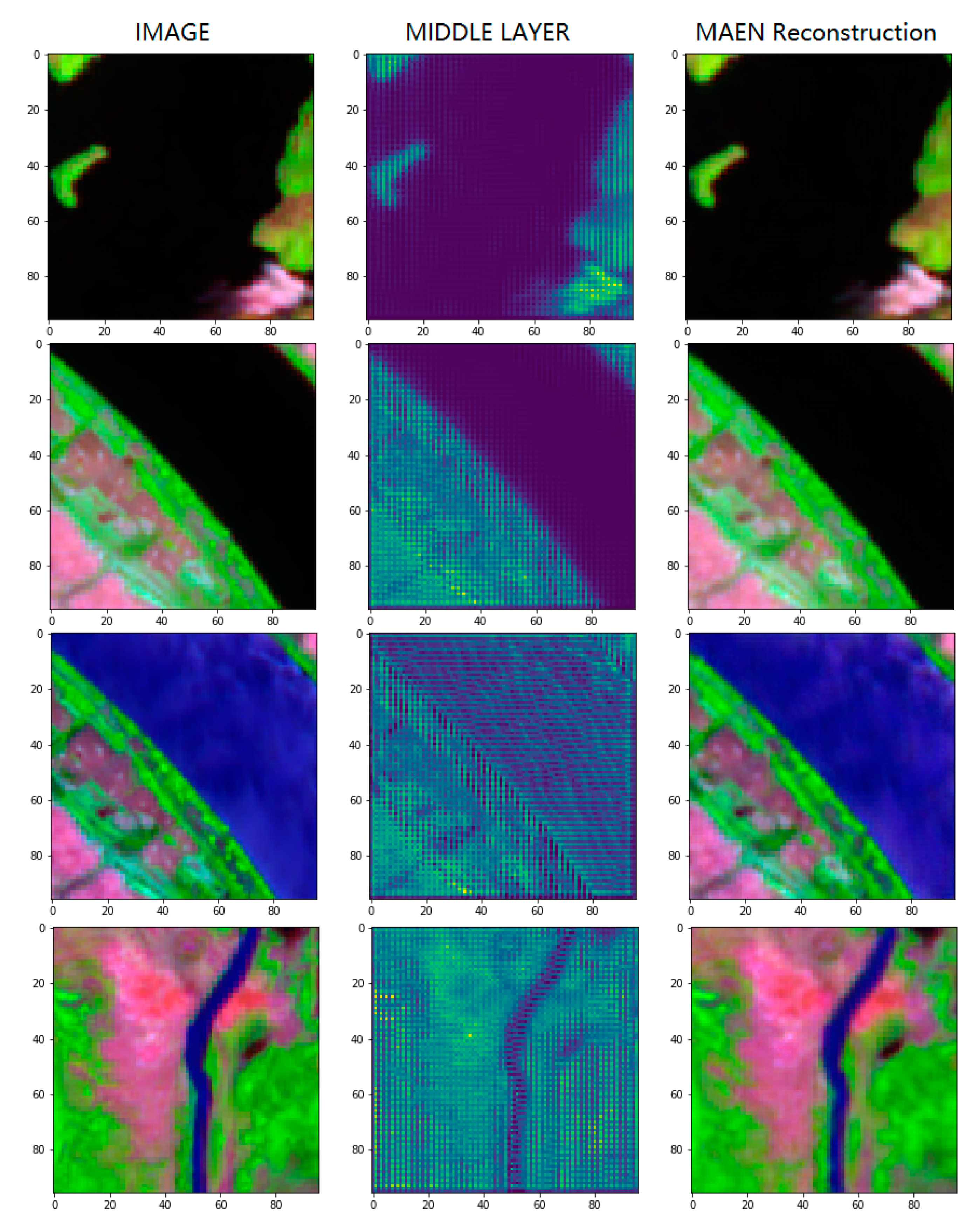
2.2.1. Semantic Feature Extraction Based on MAEN

The goal of this method is to extract an SBF from the multi-band RSIR that contains general information for each individual RSIR sample. To achieve this, the model learns to recover the input multi-band RSIR using an SBF matrix, which allows the output of the AEN to be similar to the input.

In this paper, the proposed MAEN structure is an enhancement of the standard AEN concept. In Figure 7, the AEN-9 structure corresponds to a normal AEN structure with nine convolutional layers. One possible way of improving the reconstruction ability of the AEN model is to increase the number of layers; therefore, we designed the AEN-15 model, which includes 15 convolutional layers. In the meantime, we changed the order of the layers, resulting in a multi-peak style AEN structure, which we called MAEN.

The detailed structure of MAEN in Figure 7 is shown in Figure 8. The proposed structure follows the Image AEN, which uses convolutional layers to achieve the band dimension transform. In particular, and distinct from the normal V shape AEN, whereby the series of the convolutional layer kernel sizes first gradually increases and then decreases in a V shape, we propose a multi-peak style AEN (MAEN) for the SRIR task. The MAEN structure consists of several 96 × 96 × R layers, connecting by 3 × 3 convolutional kernel.

Suppose there are X samples from the global RSIR dataset, and that each of the samples has p pixels. As described above, the aim is for the output X’ of the MAEN to be the same as X, and the middle layer output will be used in the next step, below.

2.2.2. Manifold Learning-Based Clustering

Suppose an l*m*n matrix M comprising the middle layer outputs of the MAEN, where we obtain the SBF, which is used for semantic feature clustering. The input of this step will be a l*p matrix(p = m*n). This is referred to as $M^{\prime }$, and includes $M_a{}^{\prime }$ and $M_b{}^{\prime }$ corresponding to $X_a$ and $X_b$.

To obtain more relationship information for the clustering process, the MSF matrix is first transformed by manifold learning into a higher dimensional space, resulting in an l*q matrix $M^{″}$, which includes $M_a{}^{″}$ and $M_{\mathrm{b}}{}^{″}$.

Then, the K-means-based clustering algorithm method is applied to divide $M_a{}^{″}$ into serval semantic groups, $G=(g_1,g_2,\dots ,g_i)$; the center of each group is defined as $C=(c_1,c_2,\dots ,c_i)$. Thus, the semantic relationship of X is observed using K-means clustering.

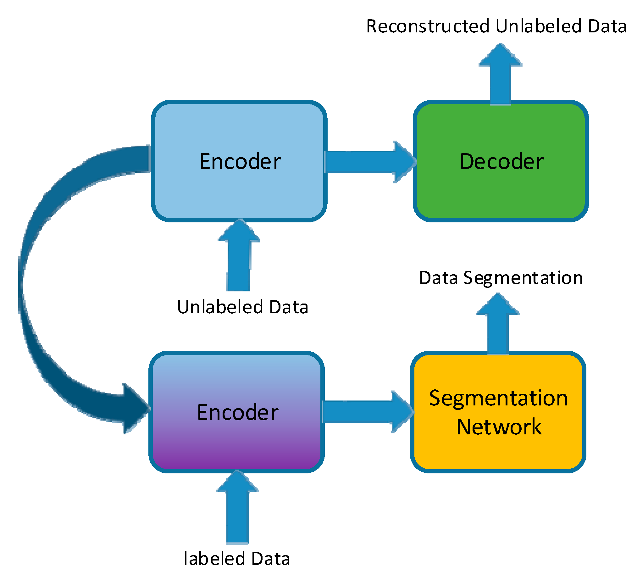
2.2.3. Semi-Supervised Learning Based on Information Transform

Based on the above-mentioned description, the semantic relationship is given in different groups as $G=(g_1,g_2,\dots ,g_i)$. To fully use the group relationship, we train multiple CNN models $D=(d_1,d_2,\dots ,d_i)$ for each group within G.

Due to the few shot issue, there may be fewer samples within a group. Thus, we propose a semi-supervised learning method for transforming additional information from unlabeled data in order to help create a model for better initialization, as shown in Figure 9. The idea is described as follows. For a segmentation CNN model waiting for training, we first only keep the encoding part of the model and build a decoding part that is symmetrical with the encoding part rebuilt with a AEN model. Then, we train this AEN model well and transform the encoding part to the segmentation CNN model for parameter initialization.

Additionally, data augmentation is applied during the training process, which shifts the sample both in the horizontal and the vertical direction.

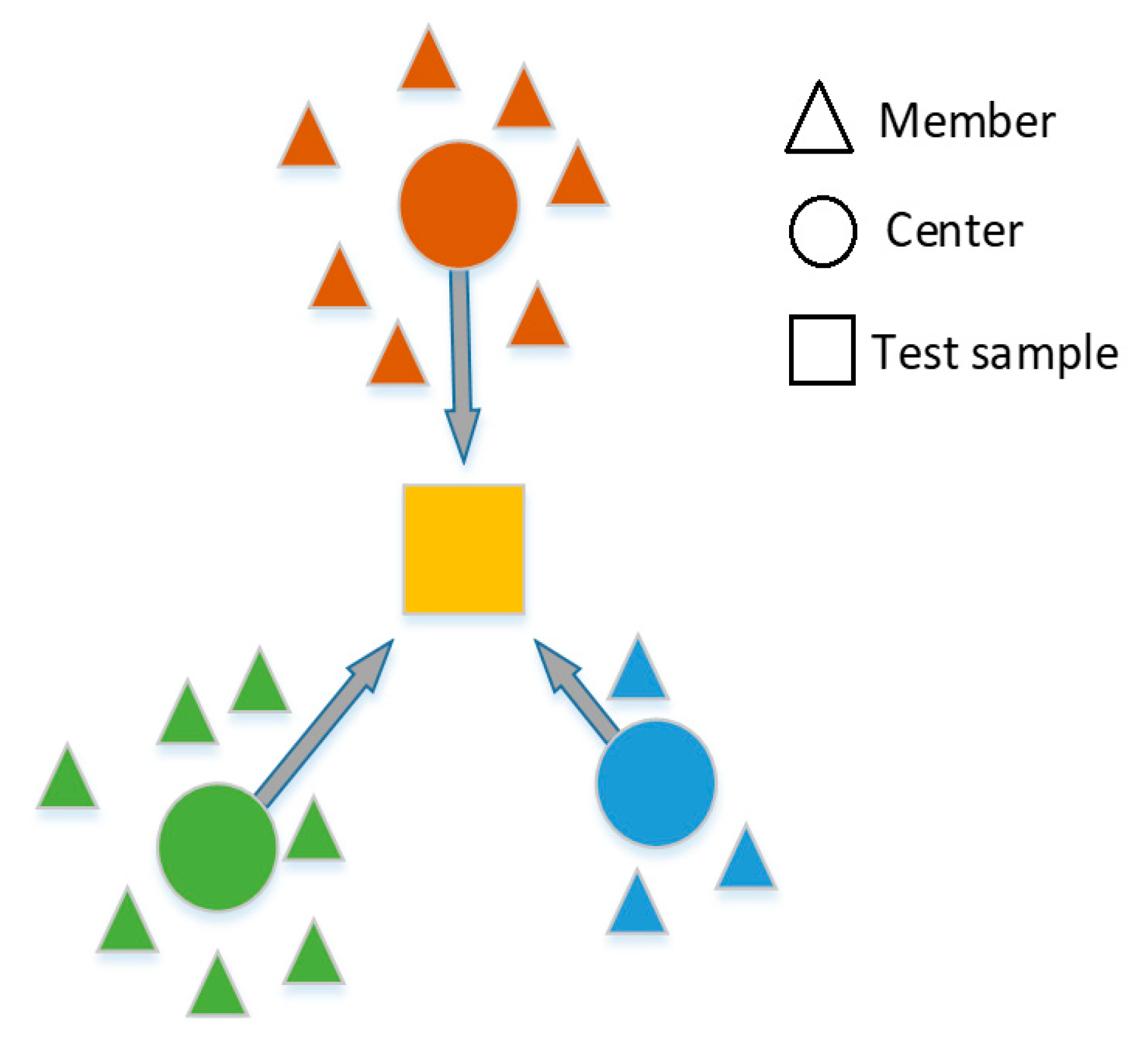
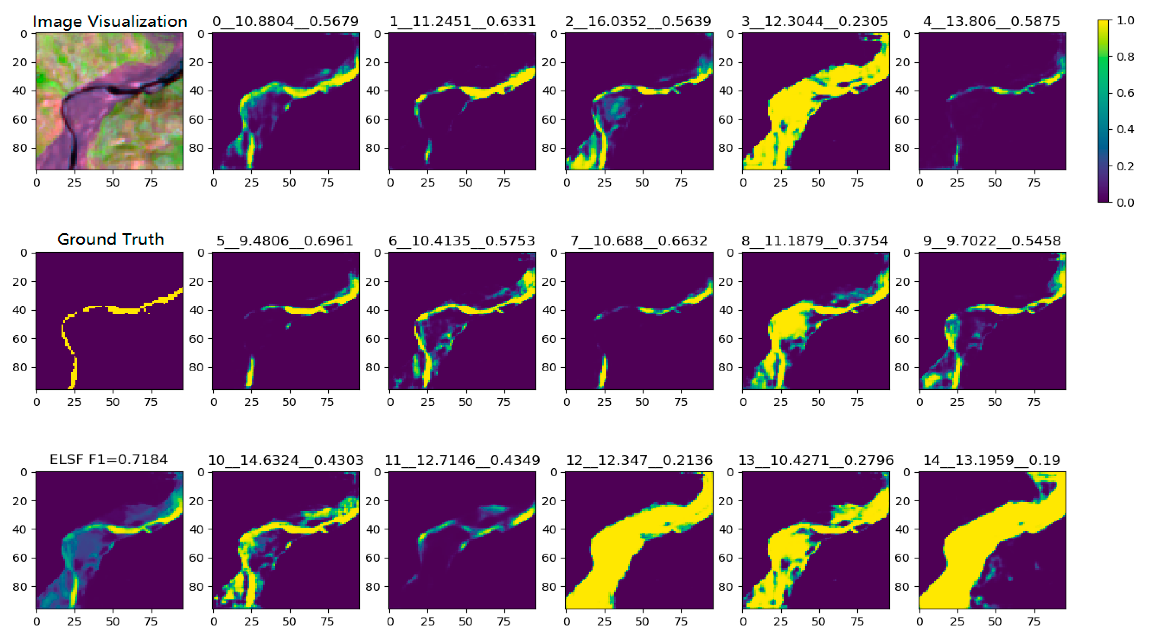
2.2.4. Ensemble Learning-Based Similarity Fusion

To segment an unlabeled RSIR sample within $X_b$, we propose an ensemble learning-based similarity fusion (ELSF) method that combines the semantic segmentation information from the semantic grouping space based on the distance.

Figure 10 shows the basic idea of measuring distances in a two-dimensional (2-D) space. In our case, the semantic space dimension N is greater than 2.

As mentioned above, in order to test a sample $X_{b_i}$ within $X_b$ for the final semantic result, we first obtain the individual output $D(X_{b_i})$ using D models. The distance $L_i\in L$ between a test sample and a group center $c_i$ is defined by (1):

$$L_i=\sqrt{{\displaystyle {\sum }_{j=0}^n{(M_b{{}^{″}}_j-c_{i_j})}^2}}$$

(1)

To obtain the weight matrix for the semantic fusion, the weight matrix $W_i\in W$ is obtained from $L_i\in L$ using a reverse softmax transform, as defined in (2):

$$W_i=\frac{{\mathrm{e}}^{-L_i}}{{\displaystyle {\sum }_{j=0}^m{\mathrm{e}}^{-L_j}}}$$

(2)

The final semantic result $F(X_b)$, which fuses $D(X_{b_i})$, is calculated using (3):

$$F(X_b)={\displaystyle {\sum }_{i=0}^m{W}_{i}D(X_{b_i})}$$

(3)

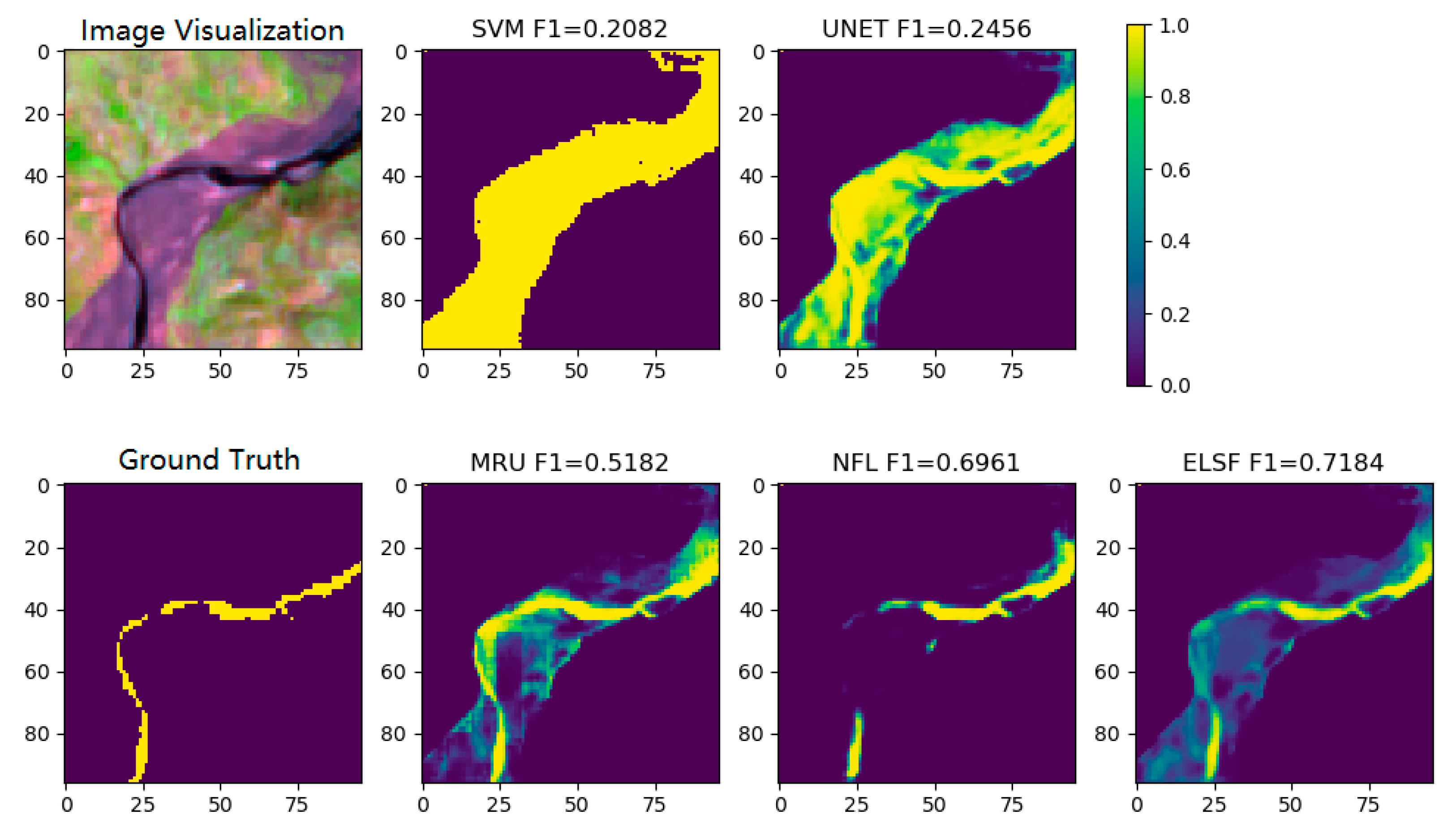
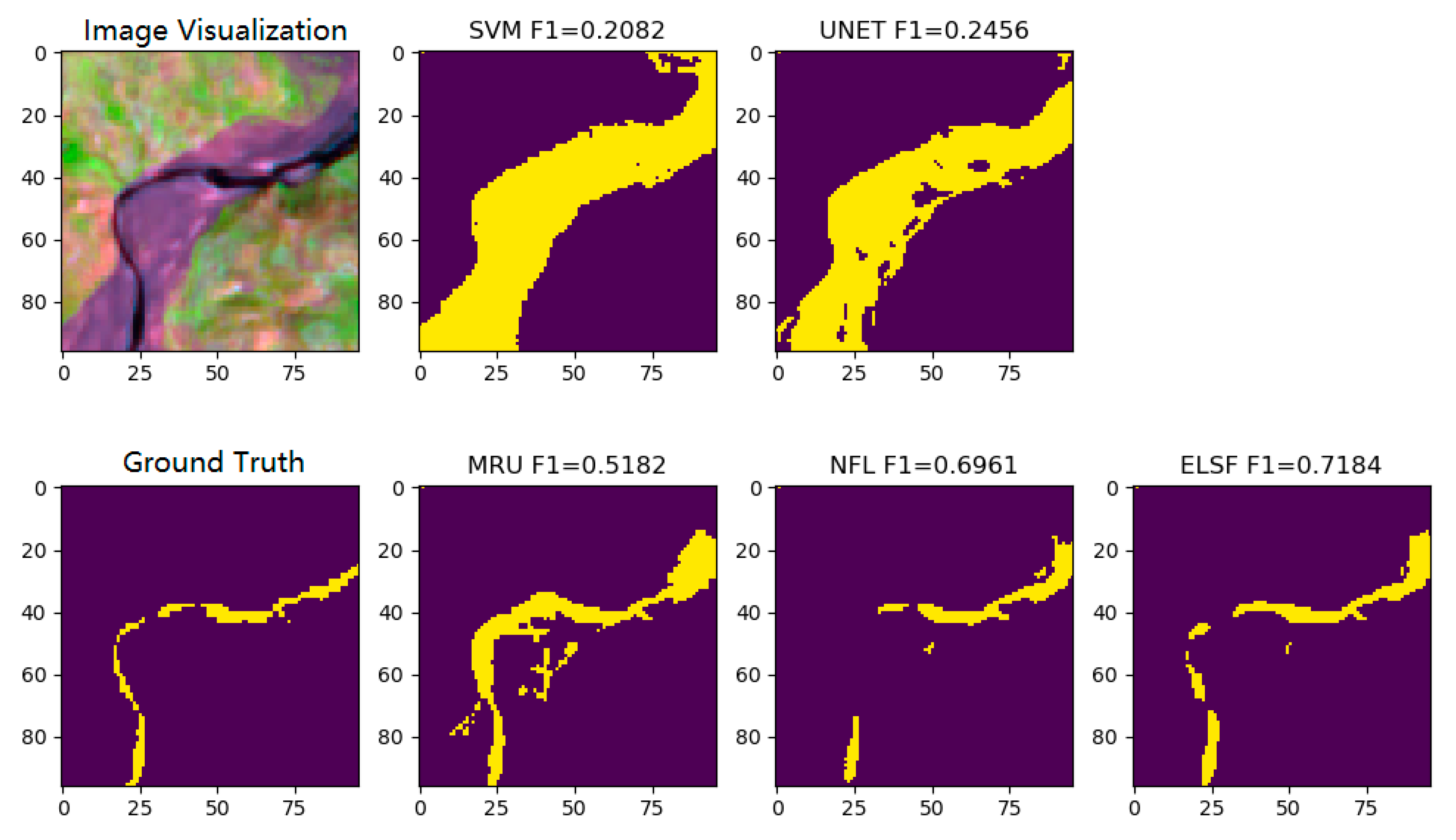
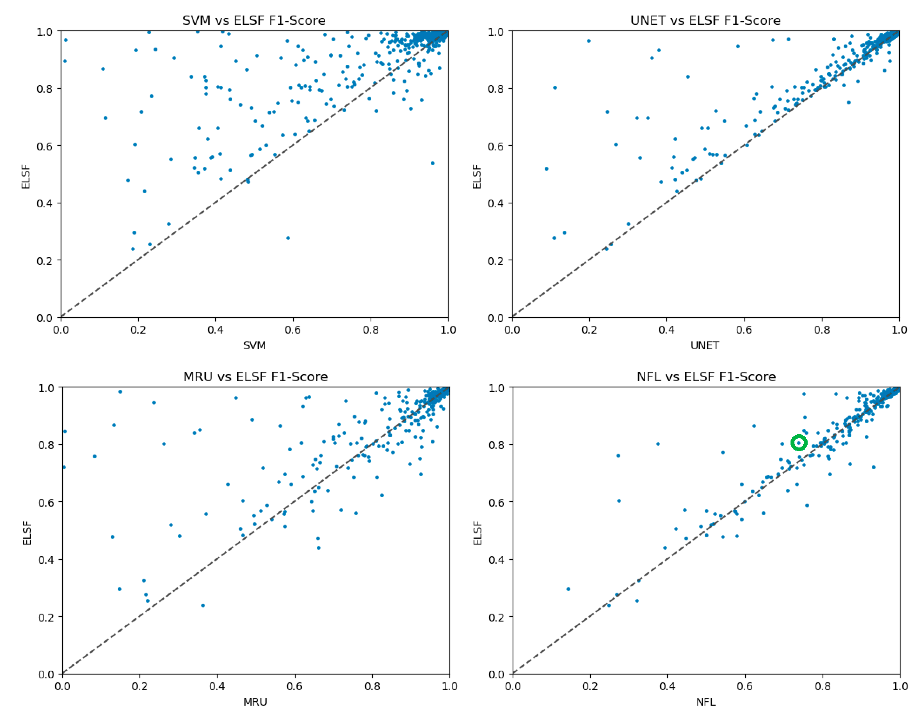
2.3. Four Algorithms (SVM, UNet, MultiResUNet, NFL) Used for Comparison with ELSF

The algorithms to be compared are SVM [42], UNet [43], MultiResUNet [44], and a non-fusion learning method (NFL) described in (4).

SVM is a traditional machine learning method that is widely used in classification tasks [45]. UNet is widely used for semantic segmentation. Other improved architectures that are based on UNet have been proposed in recent years. Here, we compare with MultiResUNet, which is a popular and state-of-the-art variant of the UNet architecture for handling multiple-resolution data.

In our proposed algorithm, the final fusion segmentation combines the segmentation from all of the group models using the ELSF method, as shown in (3). To show the efficacy of information fusion, we select an NFL method for comparison, using (4). The NFL method only considers the nearest group model during the test image segmentation, rather than combining all of the group model fusions.

$$F(X_b)=D(X_{b_i})$$

(4)

3. Results and Discussion

3.1. Experiment Setup

The training and testing processes were implemented with the Window 10 Python3 GTX2080 environment. The algorithm training parameters are shown in

Table 2. Parameters for the algorithm training processes.

Algorithm	Parameter Type	Parameter Set
SVM	Kernel Type	RBF
UNet	Learning Rate	0.0001
	Loss function	Binary Cross Entropy
MultiResUNet	Learning Rate	0.0001
	Loss function	Binary Cross Entropy
NFL	Learning Rate	0.0001
	Loss function	Binary Cross Entropy
ELSF	Learning Rate	0.0001
	Loss function	Binary Cross Entropy

. Here, we used same learning rate and loss function for the deep learning models.

3.2. Semantic Feature Extraction Based on MAEN

Figure 11 shows the semantic feature extraction results using MAEN. The reconstructed RSIR images are visualized in a false color composite style with Bands #9, #7 and #3. The semantic features are obtained from the middle layer, as shown in Figure 8. As shown in Figure 11, the MEAN is able to reconstruct the RSIR, and the semantic features are highly related to the RSIR. Furthermore, the middle layer outputs of the MAEN between the first and second row, and the third and fourth column are highly related to each other, as the river visualization colors in the RSIR images are similar. The improvement in these mapping results means that the proposed MAEN is able to extract the semantic features from the RSIR.

To validate the MAEN performance with respect to feature extraction, we further calculated the image reconstruction ability among the proposed MAEN architecture and two normal AEN architectures, AEN-9 and AEN-15, as shown in Figure 7. The image reconstruction ability is defined as follows. Suppose an m×n×p matrix A is defined as an RSIR image. Then, A is used as the AEN model input, and reconstruction image B is acquired from the AEN model output. Thus, the difference between each corresponding pixel in A and B can be used to validate the image reconstruction performance, which is calculated as follows:

$$\mathrm{Diff}(\mathrm{A},\mathrm{B})={\displaystyle {\sum }_{i=0}^m{\displaystyle {\sum }_{j=0}^n{\displaystyle {\sum }_{k=0}^p\left|{\mathrm{A}}_{i,j,k}{-\mathrm{B}}_{i,j,k}\right|}}}$$

(5)

The smaller the Diff(A, B) value, the better the image reconstruction ability. Table 2 shows the Diff(A, B) distribution using 2000 random unlabeled river samples from the proposed dataset, through different AEN model structures. For each random sample, we acquired the reconstruction image using the three AEN models, and calculated the difference using (4). Thus, for each AEN model, 2000 difference values were generated in order to measure the image reconstruction ability. Then, we first sorted the 2000 difference values of each AEN model, and calculated the average and the median for each AEN model. The smaller the average value and the median, the better the image reconstruction ability.

Table 3. Image reconstruction performance.

AEN Model	Distribution Value
	Average	Median
AEN-9	6215.76	4120.43
AEN-15	4109.92	2052.95
MAEN	3778.49	1540.60

shows the distribution of difference values.

As shown in Table 3, the average and the median for the Diff(A, B) of the AEFCNN model is smaller than for the two normal AEN models, which demonstrates the image reconstruction performance of the purposed AEFCNN model. Furthermore, AEN-15 is better than AEN-9 based on the distribution value. The reason that AEN-15 has better reconstruction performance than AEN-9 is the increase in the number of layers. One possible reason for MAEN being better than AEN-15 could be the multi-peak style of the layers, which is the significant difference between MAEN and the normal AEN models. The multi-peak style structure transforms the feature into a different shape, allowing the middle layers’ output to become more stable.

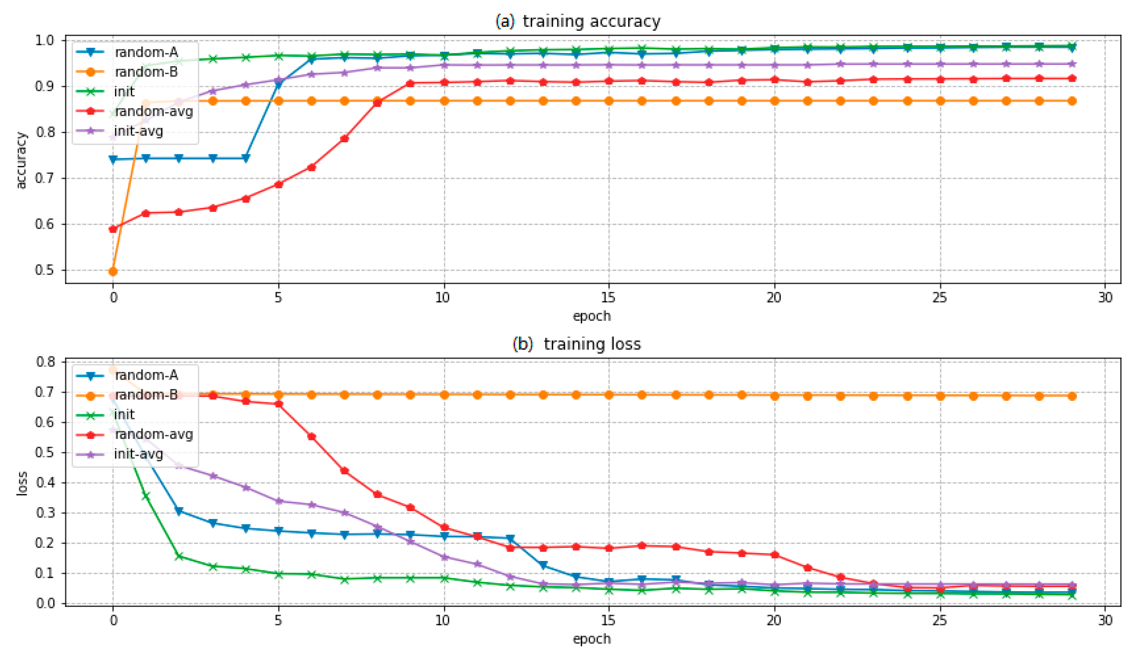
3.3. Semi-Supervised Learning Based on Information Transform

The semi-supervised learning pre-trained method is compared with a non-initialized (random) pre-trained method. Figure 12 shows the training accuracy and loss curves during the model training process.

We repeated training for the models 10 times with different parameter initialization methods, and selected the most common situations, along with the statistical average curves. The ‘random-A’ curve represents a training process result with a reasonable loss, and the segmentation result is close to the training set. The ‘random-B’ curve represents a training process that results in a badly trained model in which the loss is not low enough to segment the RSIR training samples. The ‘init’ curve shows a training process using the semi-supervised learning pre-trained method, resulting in a good model that segments the RSIR training samples well. The ‘random-avg’ and ‘init-avg’ curves represent the average performance, and show a similar trend to that of the individual separate results. Above all, the results show that the semi-supervised learning pre-trained method helps the training process by managing the local minimum.

3.4. Global River Segmentation

We compared the proposed ELSF method, with SVM, UNet, MultiResUNet, and NFL methods using the proposed dataset, including 2265 samples for training, and 616 samples for testing, following an 80% training and 20% testing rule through seed-based random selection. In addition, we applied 10-fold cross-validation on the training set for model validation. Furthermore, in order to avoid overfitting during the model training process, the drop-out technique was incorporated into the models. The idea of this technique is to randomly drop units from the neural network during training, thereby avoiding model overfitting [46].

Specifically, during the training and validation process, the average precision of the 10-fold cross-validation for the proposed ELSF method was 93.24%, thus proving the stability of the proposed ELSF model.

Next, we will explain the detail of the semantic fusion results during the testing process.

Figure 13 shows the semantic fusion process of ELSF method with a test sample. Each subplot represents a test sample segmentation result that uses different clustering trained CNN model. Each subtitle contains the information as ‘Group-ID__TestSample-to-Center-Distance__F1-score’.

For this test sample, Group-ID #5 shows the shortest distance between the test sample and the clustering group center. The F1-score of the segmentation result using this model is 0.696, which is the highest score among the groups, and shows the correlation between the semantic distance and the distance-based segmentation performance. The NFL method F1-score of this test sample is taken from the closest model, which is Group-ID #5, as shown in Figure 14. The ELSF method aims to combine the segmentation results from all the models in order to gather all of the information in a reasonable way. The ELSF result shows the F1-score for 0.7184, and the improvement can be seen in the center part of these RSIR samples, compared with the other segmentation results in Figure 14.

Figure 15 shows the binary results of the same test sample from Figure 13 and Figure 14. Since the CNN model output is a value that ranges from 0 to 1, we consider values higher than 0.5 to be water pixels, and those equal to or lower than 0.5 to be land pixels. Then, we are able to calculate the F1-score using the segmentation results of different methods according to the ground-truth label of the test sample.

We also compare the F1-score of the proposed ELSF method with other methods, as shown in Figure 16. Each point within the scatterplot figure represents the F1-scores of a test sample using ELSF and a comparison method. The more the points are located on the top-left side of the diagonal dotted line, the better the performance the ELSF in comparison with the comparison method. In the SVM vs. ELSF and UNet vs. ELSF scatterplots, ELSF performs significantly better than the compared methods. In the MultiResUNet vs. ELSF scatterplot, although the architecture improvement exists from UNet to MultiResUNet, still more than half of the points have a higher F1-score in the UNet-based ELSF, when compared with MultiResUNet. In the NFL vs. ELSF scatterplot, it can be seen that the points are mainly located near the diagonal dotted line. Additionally, in the top-right corner of the NFL vs. ELSF scatterplot, slightly more points appear on the top-left side of the diagonal dotted line. Additionally, the point within the green circle represents a testing sample coming from the eastern coast of Brazil; this region does not appear in the training set, and the ELSF model has the better F1-score than the comparison models for this sample. This proves that compared to NFL, the idea of the ELSF adding the space information of the surrounding semantic models into the segmentation process helps with the RSIR segmentation task.

Finally, the average performance of the proposed ELSF method and other comparison methods is shown in

Table 4. Comparison of segmentation among different algorithms.

Algorithm	Precision	Recall	F1
SVM	85.61	95.61	87.63
UNet	90.42	95.71	91.27
MultiResUNet	92.56	94.03	91.59
NFL	92.01	95.73	92.76
ELSF	92.84	95.82	93.32

. The results show that the NFL performs better than the UNet and UNet-based MultiResUNet. NFL is better able to learn the semantic information from a similar RSIR clustering deep learning model. Furthermore, the proposed ELSF outperforms the other methods, because ELSF is able to combine the information from each semantic RSIR clustering deep learning model, and NFL only contains the closest clustering model information. Thus, similar semantic information being located in all the semantic groups helps the segmentation process of the ELSF method.

4. Conclusions

We first presented an AEN-based semantic feature extraction structure. Then, a clustering-based semantic process method was proposed in order to achieve better RSIR sample grouping. Thirdly, a semi-supervised learning method based on information transformation was proposed to better initialize the CNN model with the aim of improving the convergence rate with a minimum of local handling. Finally, a similarity-based fusion method for global RSIR segmentation based on trained CNN models was proposed with the aim of achieving a better segmentation result.

Most importantly, we proposed a framework for solving the segmentation challenge for various types of RSIR at a global scale. The paper provides a solution that reasonably combines the semantic information used for segmentation, and an enhanced training technique based on semi-supervision to better handle local minima. Better ELSF performance can be expected, and river monitoring research can be set up over long periods of time if larger numbers of ground-truth samples are available for clustering and training process. Furthermore, higher spatial and temporal resolution satellite data such as World View-2(WV2) data may help to achieve river mapping at higher resolution. This needs to be explored through further research.

References

1. Pekel, J.-F.; Cottam, A.; Gorelick, N.; Belward, A.S. High-resolution mapping of global surface water and its long-term changes. Nature 2016, 540, 418–422. [Google Scholar] [CrossRef] [PubMed]
2. Wu, C.L.; Chau, K.W. Prediction of rainfall time series using modular soft computingmethods. Eng. Appl. Artif. Intel. 2013, 26, 997–1007. [Google Scholar] [CrossRef] [Green Version]
3. Mueller, N.; Lewis, A.; Roberts, D.; Ring, S.; Melrose, R.; Sixsmith, J.; Lymburner, L.; Mclntyre, A.; Tan, P.; Curnow, S.; et al. Water observations from space: Mapping surface water from 25 years of Landsat imagery across Australia. Remote Sens. Environ. 2016, 174, 341–352. [Google Scholar] [CrossRef] [Green Version]
4. Tweed, S.; Marc, L.; Ian, C. Groundwater–surface water interaction and the impact of a multi-year drought on lakes conditions in South-East Australia. J. Hydrol. 2009, 379, 41–53. [Google Scholar] [CrossRef]
5. Zhang, T.; Zhang, X.N.; Xia, D.Z.; Liu, Y.Y. An Analysis of Land Use Change Dynamics and Its Impacts on Hydrological Processes in the Jialing River Basin. Water 2014, 6, 3758–3782. [Google Scholar] [CrossRef] [Green Version]
6. Akbari, M.; Torabi Haghighi, A.; Aghayi, M.M.; Javadian, M.; Tajrishy, M.; Kløve, B. Assimilation of satellite-based data for hydrological mapping of precipitation and direct runoff coefficient for the Lake Urmia Basin in Iran. Water 2019, 11, 1624. [Google Scholar] [CrossRef] [Green Version]
7. Homsi, R.; Shiru, M.S.; Shahid, S.; Ismail, T.; Harun, S.B.; Al-Ansari, N.; Yaseen, Z.M. Precipitation projection using a cmip5 gcm ensemble model: A regional investigation of syria. J. Eng. Appl. Comp. Fluid. 2020, 14, 90–106. [Google Scholar] [CrossRef]
8. Duro, D.C.; Coops, N.C.; Wulder, M.A.; Han, T. Development of a large area biodiversity monitoring system driven by remote sensing. Prog. Phys. Geog. 2007, 31, 235–260. [Google Scholar] [CrossRef]
9. Alsdorf, D.E.; Rodriguez, E.; Lettenmaier, D.P. Measuring surface water from space. Rev. Geophys. 2007, 45, 1–24. [Google Scholar] [CrossRef]
10. Nourani, V.; Ghasemzade, M.; Mehr, A.D.; Sharghi, E. Investigating the effect of hydroclimatological variables on urmia lake water level using wavelet coherence measure. J. Water Clim. Chang. 2019, 10, 13–29. [Google Scholar] [CrossRef] [Green Version]
11. Gleason, C.J.; Smith, L.C. Toward global mapping of river discharge using satellite images and at-many-stations hydraulic geometry. Proc. Natl. Acad. Sci. USA 2014, 111, 4788–4791. [Google Scholar] [CrossRef] [PubMed] [Green Version]
12. Isikdogan, F.A.; Bovik, C.; Passalacqua, P. Surface water mapping by deep learning. IEEE J. Sel. Top. Appl. Earth Observ. Remote Sens. 2017, 10, 4909–4918. [Google Scholar] [CrossRef]
13. Haas, E.M.; Bartholomé, E.; Combal, B. Time series analysis of optical remote sensing data for the mapping of temporary surface water bodies in sub-Saharan western Africa. J. Hydrol. 2009, 370, 52–63. [Google Scholar] [CrossRef]
14. Gao, B.C. NDWI–A normalized difference water index for remote sensing of vegetation liquid water from space. Remote Sens. Environ. 1996, 58, 257–266. [Google Scholar] [CrossRef]
15. McFeeters, S.K. The use of normalized difference water index (NDWI) in the delineation of open water features. Int. J. Remote Sens. 1996, 17, 1425–1432. [Google Scholar] [CrossRef]
16. Xu, H.Q. A study on information extraction of water body with the modified normalized difference water index (MNDWI). J. Remote Sens. 2005, 9, 589–595. [Google Scholar]
17. Du, Y.; Zhang, Y.; Ling, F.; Wang, Q.; Li, W.; Li, X. Water bodies’ mapping from sentinel-2 imagery with modified normalized difference water index at 10-m spatial resolution produced by sharpening the SWIR band. Remote Sens. 2016, 8, 354. [Google Scholar] [CrossRef] [Green Version]
18. Zhu, Z.; Wang, S.; Woodcock, C.E. Improvement and expansion of the Fmask algorithm: Cloud cloud shadow and snow detection for Landsats 4–7 8 and Sentinel 2 images. Remote Sens. Environ. 2015, 159, 269–277. [Google Scholar] [CrossRef]
19. Shamshirband, S.; Hashemi, S.; Salimi, H.; Samadianfard, S.; Asadi, E.; Shadkani, S.; Mosavi, A.; Naipour, N. Predicting Standardized Streamflow index for hydrological drought using machine learning models. J. Eng. Appl. Comp. Fluid. 2019, 14, 339–350. [Google Scholar] [CrossRef]
20. Melgani, F.; Bruzzone, L. Classification of hyperspectral remote sensing images with support vector machines. IEEE Trans. Geosci. Remote Sens. 2004, 42, 1778–1790. [Google Scholar] [CrossRef] [Green Version]
21. ShieYui, L.; Sivapragasam, C. Flood Stage Forecasting With Support Vector Machines. J. Am. Water. Resour. As. 2002, 38, 173–186. [Google Scholar]
22. Asefa, T.; Kemblowski, M.; Lall, U.; Urroz, G. Support vector machines for nonlinear state space reconstruction: Application to the great salt lake time series. Water Resour. Res. 2005, 41, 1–10. [Google Scholar] [CrossRef] [Green Version]
23. Pal, M. Ensemble learning with decision tree for remote sensing classification. World Acad. Sci. Eng. Technol. 2007, 36, 258–260. [Google Scholar]
24. Huang, H.; Liang, Z.; Li, B.; Wang, D.; Li, Y. Combination of multiple data-driven models for long-term monthly runoff predictions based on bayesian model averaging. Water Resour. Manag. 2019, 33, 3321–3338. [Google Scholar] [CrossRef]
25. Tyralis, H.; Papacharalampous, G.; Tantanee, S. How to explain and predict the shape parameter of the generalized extreme value distribution of streamflow extremes using a big dataset. J. Hydrol. 2019, 574, 628–645. [Google Scholar] [CrossRef]
26. Bhuiyan, M.A.E.; Nikolopoulos, E.I.; Anagnostou, E.N.; Quintana-Seguí, P.; Barella-Ortiz, A. Anonparametric statistical technique for combining global precipitation datasets: Development and hydrological evaluationover the iberian peninsula. Hydrol. Earth Syst. Sci. 2018, 22, 1371–1389. [Google Scholar] [CrossRef] [Green Version]
27. Ehsan, B.M.A.; Begum, F.; Ilham, S.J.; Khan, R.S. Advanced wind speed prediction using convective weather variables through machine learning application. Comput. Geosci-UK 2019, 1, 1–9. [Google Scholar]
28. Jia, X.W.; Khandelwal, A.; Mulla, D.J.; Pardey, P.G.; Kumar, V. Bringing automated, remote-sensed, machine learning methods to monitoring crop landscapes at scale. Agric. Econ. Czech. 2019, 50, 41–50. [Google Scholar] [CrossRef]
29. Kussul, N.; Lavreniuk, M.; Skakun, S.; Shelestov, A. Deep learning classification of land cover and crop types using remote sensing data. IEEE Geosci. Remote Sens. Lett. 2017, 14, 778–782. [Google Scholar] [CrossRef]
30. Zhang, S.; Wu, R.; Xu, K.; Wang, J. R-CNN-Based Ship Detection from High Resolution Remote Sensing Imagery. Remote Sens. 2019, 11, 631. [Google Scholar] [CrossRef] [Green Version]
31. Mou, L.; Bruzzone, L.; Zhu, X.X. Learning spectral-spatial-temporal features via a recurrent convolutional neural network for change detection in multispectral imagery. IEEE Trans. Geosci. Remote Sens. 2019, 57, 924–993. [Google Scholar] [CrossRef] [Green Version]
32. Zhang, D.; Peng, Q.; Lin, J.; Wang, D.; Liu, X.; Zhuang, J. Simulating Reservoir Operation Using a Recurrent Neural Network Algorithm. Water 2019, 11, 865. [Google Scholar] [CrossRef] [Green Version]
33. Taormina, R.; Chau, K.W. ANN-based interval forecasting of streamflow discharges using the LUBE method and MOFIPS. Eng. Appl. Artif. Intel. 2014, 45, 429–440. [Google Scholar] [CrossRef]
34. Zhong, Z.; Li, J.; Luo, Z.; Chapman, M. Spectral–spatial residual network for hyperspectral image classification: A 3-D deep learning framework. IEEE Trans. Geosci. Remote Sens. 2018, 56, 847–858. [Google Scholar] [CrossRef]
35. Miao, Z.; Fu, K.; Sun, H.; Sun, X.; Yan, M. Automatic water-body segmentation from high-resolution satellite images via deep networks. IEEE Geosci. Remote Sens. Lett. 2018, 15, 602–606. [Google Scholar] [CrossRef]
36. Fu, G.; Liu, C.; Zhou, R.; Sun, T.; Zhang, Q. Classification for High Resolution Remote Sensing Imagery Using a Fully Convolutional Network. Remote Sens. 2017, 9, 498. [Google Scholar] [CrossRef] [Green Version]
37. Yu, L.; Wang, Z.; Tian, S.; Ye, F.; Ding, J.; Kong, J. Convolutional neural networks for water body extraction from Landsat imagery. Int. J. Comput. Intell. Appl. 2017, 16, 1750001. [Google Scholar] [CrossRef]
38. Sunaga, Y.; Natsuaki, R.; Hirose, A. Land form classification and similar land-shape discovery by using complex-valued convolutional neural networks. IEEE Trans. Geosci. Remote Sens. 2019, 57, 7907–7917. [Google Scholar] [CrossRef]
39. Liu, B.; Yu, X.; Yu, A.; Zhang, P.; Wan, G.; Wang, R. Deep few-shot learning for hyperspectral image classification. IEEE Trans. Geosci. Remote Sens. 2019, 57, 2290–2304. [Google Scholar] [CrossRef]
40. Song, W.; Wang, L.; Liu, P.; Choo, K.K.R. Improved t-SNE based manifold dimensional reduction for remote sensing data processing. Multimed Tools Appl. 2019, 78, 4311–4326. [Google Scholar] [CrossRef]
41. Dhanachandra, N.; Manglem, K.; Chanu, Y.J. Image segmentation using K-means clustering algorithm and subtractive clustering algorithm. Procedia. Comput. Sci. 2015, 54, 764–771. [Google Scholar] [CrossRef] [Green Version]
42. Guo, X.; Huang, X.; Zhang, L.; Zhang, L.; Plaza, A.; Benediktsson, J.A. Support tensor machines for classification of hyperspectral remote sensing imagery. IEEE Trans. Geosci. Remote Sens. 2016, 54, 3248–3264. [Google Scholar] [CrossRef]
43. Ronneberger, O.; Fischer, P.; Brox, T. U-net: Convolutional networks for biomedical image segmentation. In International Conference on Medical Image Computing and Computer-Assisted Intervention; Spring: Cham, Switzerland, 2015; Volume 9351, pp. 234–241. [Google Scholar]
44. Ibtehaz, N.; Rahman, M.S. MultiResUNet: Rethinking the U-Net architecture for multimodal biomedical image segmentation. Neural Netw. 2020, 121, 74–87. [Google Scholar] [CrossRef] [PubMed]
45. Maulik, U.; Chakraborty, D. Remote sensing image classification: A survey of support-vector-machine-based advanced techniques. IEEE Geosci. Remote Sens. Mag. 2017, 5, 33–52. [Google Scholar] [CrossRef]
46. Srivastava, N.; Hinton, G.; Krizhevsky, A.; Sutskever, I.; Salakhutdinov, R. Dropout: A Simple Way to Prevent Neural Networks from Overfitting. J. Mach. Learn. Res. 2014, 15, 1929–1958. [Google Scholar]
Figure 1. Different representation of RSIR from same location among times: (a) March 21, 2016, (b) August 18, 2016, (c) November 16, 2016.
Water 12 02258 g001
Figure 2. Distribution of the collected global river dataset (the black circle located in the Northern part of South America will be further visualized in Figure 3).
Water 12 02258 g002
Figure 3. Detail of the location and construction for a typical river (Each dot represents a small piece of river, and the cyan bounding box of each dot represents the coverage area of each image within our dataset).
Water 12 02258 g003
Figure 4. Example of the sample visualization and manual ground truth in the dataset.
Water 12 02258 g004
Figure 5. Example of different categories of river type from the dataset: (a) River type category 1, (b) River type category 2.
Water 12 02258 g005
Figure 6. The proposed semantic fusion structure (the structure contains a model training process and river segmentation process, including sematic feature extraction and sematic segmentation fusion methods).
Water 12 02258 g006
Figure 7. The proposed MAEN structure and comparison with the normal AEN structure (AEN-9, AEN-15).
Water 12 02258 g007
Figure 8. Construction of the proposed MAEN. The middle layer output is extracted as a semantic feature.
Water 12 02258 g008
Figure 9. Proposed semi-supervised learning process. The information from the unlabeled data-trained AEN is used to supervise the labeled data-trained CNN process.
Water 12 02258 g009
Figure 10. Proposed segmentation fusion method. The final segmentation is fusion using multiple semantic groups (the red, blue and green colors represent different semantic grouping spaces, the yellow square represents the final segmentation result).
Water 12 02258 g010
Figure 11. Figures of RSIR image visualization (column 1). Semantic features from the middle layer of the MAEN (column 2). MAEN image reconstruction (column 3) during the training process.
Water 12 02258 g011
Figure 12. Figures of (a) training accuracy curves and (b) training loss curves using different supervised learning algorithms.
Water 12 02258 g012
Figure 13. Figures of the tested RSIR sample visualization, ground truth, ELSF method (column 1). Segmentation results from each individual group training CNN model. The sub-titles represent Group-ID__TestSample-to-Center-Distance__F1-Score (column 2 to column 6).
Water 12 02258 g013
Figure 14. Figures of sample visualization, SVM, UNet segmentation fraction results (row 1), sample ground truth, MultiResUNet, NFL, ELSF segmentation fraction results (row 2).
Water 12 02258 g014
Figure 15. Figures of sample visualization, SVM, UNet segmentation binary results (row 1), sample ground truth, MultiResUNet, NFL, ELSF segmentation fraction results (row 2).
Water 12 02258 g015
Figure 16. F1-score comparison between different algorithms. (Each point within a scatterplot figure represents the F1-score of a test sample using ELSF and a comparison algorithm. The point within the green circle represents a testing sample coming from the eastern coast of Brazil, a region that does not appear in the training set).
Water 12 02258 g016