A Novel Lazy Serpent Algorithm for the Prioritization of Leak Repairs in Water Networks

Abstract

Maximizing benefit from budget allocation is a major challenge for municipalities in the modern era. This is especially significant when it comes to infrastructure network management such as water distribution networks. The main challenges of water distribution networks are leakage and leak repairs. Municipalities commonly use first-in-first-out approaches to determine which leaks to allocate budget for first. Yet, the deterioration of leaks is not linear through time and requires a more in-depth assessment of the condition of the leak. Therefore, this article presents two prioritization approaches for the scheduling of leaks while incorporating deterioration over time. This paper proposes and compares two optimization techniques: (1) a well-known genetic algorithm and (2) a novel approach named the Lazy Serpent Algorithm. The Lazy Serpent Algorithm has proved capable of surpassing the genetic algorithm in determining a more optimal order by using much less computation time. The Lazy Serpent Algorithm helps municipalities better distribute their resources to maximize their desired benefits.

1. Introduction

The concept of lazy serpent was inspired by the problem of leak repair scheduling and resource allocation for repair projects. Thus, in this report leak repair projects are considered independent events, i.e., unrelated to each other. Moreover, all leaks are assumed to be deteriorating at an individual rate determined by each case and through historical data. Accordingly, in this section, previous work on scheduling optimization approaches of independent events under constraints are discussed. Some researchers attempted to distinguish independent event scheduling approaches from regular scheduling and dubbed them the name “priority algorithms.” Davis [1] identified priority algorithms and their role in solving scheduling problems. The report identified multiple algorithms capable of solving prioritization problems, mainly greedy algorithms, genetic algorithms, adaptive priority algorithms, and dynamic programming. The author also distinguished between fixed priority algorithms and adaptive priority algorithms. An early approach for optimizing independent event schedules was presented by Colorni et al. [2]. Their proposed approach used evolutionary genetic algorithms (GAs) to solve the timetable problem. This problem is limited by school hour constraints and teacher schedule constraints and the objective was to remove conflicts in classrooms and to remove the course overlaps. The authors simulated the problem as a multiconstrained, non-deterministic polynomial hard (NP-hard), combinatorial optimization problem. Using a genetic algorithm with local search as well as genetic algorithms without local search, the authors concluded that the genetic algorithm presents more flexibility in defining constraints and outperforms handmade timetables and simulated annealing timetables. Scheduling problems can be solved using a resource-driven model that is capable of optimizing the schedules of linear projects by utilizing a dynamic programming formulation and heuristic rules, as proposed by Moselhi and Hassanein [3]. The model accommodates repetitive and nonrepetitive optimization activities to develop practical and near-optimal schedules. Software was developed to embody the theoretical concepts of the model and develop case studies. The model has proved to be capable of optimizing construction time, cost, or both under a cost-plus-time bidding environment. Elshaboury et al. [4] proposed a single-objective optimization model designated for budget allocation of water repair works. In this regard, the optimization model was designed to accommodate the cost of repair strategies and the structural condition of the overall network. A comparative analysis was carried out to evaluate the performances of the modified invasive weed optimization algorithm, particle swarm optimization algorithm, shuffled frog leaping algorithm, and artificial bee colony algorithm. It was found that the modified invasive weed optimization provided better overall performance with reference other metaheuristics.

Prioritization models are required not only to prioritize but also to optimize expenditure and cost [5]. Recently, the concept of merging wireless sensor networks with optimization techniques in smart cities is gaining traction in the scientific field [6,7,8]. Existing models can be classified into two categories: (1) probabilistic and (2) nonprobabilistic approaches. When implementing a probabilistic approach, the user must collect the distribution of a given event and then utilize its distribution form to create assessments and simulation using Monte Carlo simulation [9,10,11,12,13]. On the other hand, nonprobabilistic methods utilize arithmetic laws, rules, and optimization to handle uncertainties. Nonprobabilistic approaches include fuzzy set theory, interval probabilities, and imprecise reliability [14,15,16]. For example, Morcous and Lounis [17] presented a model that is capable of minimizing the life-cycle cost of infrastructure by predicting deterioration in infrastructure networks using genetic algorithms and Markov chain networks. This model is important in this research as it shows previous work predicting and assessing multiple maintenance alternatives for a specific network within a specific timeline. To prioritize independent events, a scale of measurement is required. Elbehairy et al. [18] introduced a repair prioritization approach for bridge deck repairs. Two evolutionary algorithms are used in this approach to optimize the order within the repair schedule. These two algorithms are genetic algorithms and shuffled frog leaping algorithms. Each repair event is identified by three aspects as follows: (1) expected deterioration, (2) cost, and (3) repair impact. This research concluded that both optimization approaches are equally suitable to optimize bridge repair schedules. Another prioritization model, this time for pipe replacement prioritization, was presented by Giustolisi and Berardi [19]. The authors identify three main aspects of leak repair: (1) economic, (2) reliability, and (3) water quality. The main aim of the model is to develop a plan that maximizes the effectiveness of each pipe rehabilitation to help the decision-maker identify how to tackle the replacement plans within an infrastructure network. The primary tool for the development of this model was a multiobjective evolutionary optimization with the best results obtained when the multiobjective genetic algorithm is utilized. The research above proves the need for an approach that can help the decision-maker plan for the long-term changes within multiple similar projects. A dedicated approach for the prioritization of events—specifically leaks—and the assessment of the best manner to allocate available resources is currently not directly present. GAs are frequently used in the field of schedule optimization. Researchers have presented multiple possibilities with evolutionary algorithms capable of providing multiobjective solutions for complicated problems, e.g., scheduling and event prioritization problems. Cai and Li [20] proposed genetic algorithms to solve a scheduling problem. They presented a multiobjective genetic algorithm to optimize the schedule of 624 staff members based on three predefined criteria by the user. The algorithm proved effective in organizing shifts, optimizing the schedule, and reducing the costs by decreasing the required number of staff members to 593 individuals. The research works reviewed in this section and those presented earlier show that evolutionary algorithms in general, and specifically genetic algorithms, offer a feasible and practical solution to scheduling problems and are capable of providing adequate and reliable optimal schedules. On the other hand, evolutionary algorithms can be time-consuming as they are not explicitly designed to solve scheduling problems. In the field of single event prioritization, multiple contributions have been made, using evolutionary learning algorithms and more specifically genetic algorithms. Although beneficial and powerful, genetic algorithms have drawbacks in terms of computational efficiency and time efficiency. Evolutionary algorithms are considered time-consuming and might deflect away from the optimum solution to near-optimal solutions [1]. Additionally, evolutionary algorithms can be inefficient in handling large numbers of events without affecting their computational performance and lowering their respective speed [2]. Finally, most evolutionary algorithms tend to utilize static schedules to create optimally prioritized schedules. However, in the case of prioritizing leak repairs, there is a need for more dynamic approaches to consider the worsening of the condition of a leak that is to be repaired. Therefore, an algorithm with minimal simulation and prediction capabilities to prioritize events as they move through time is highly needed [21].

Accordingly, the objectives of this article are to (1) present a novel decision-making approach for the assessment of changing events through time, (2) present a comparative genetic algorithm model that serves the same purpose, and (3) apply both models to a given case study and compare their results.

The article is divided into four main sections. The second section introduces the methods used and the implementation approach for the article. The third section presents and compares the results. The final section presents the conclusions and the lessons learned from this research work.

2. Methodology and Implementation

This article proposes a new prioritization algorithm with a three-dimensional approach to tackle the leak prioritization problem. Figure 1 presents the model for the Lazy Serpent Algorithm presented in this article. To develop the Lazy Serpent Algorithm, research is needed in terms of simulation techniques and optimization algorithms. The primary purpose of having a background simulation technique is to predict the behavior of the leak (event) as time progresses, whereas optimization algorithms are utilized to determine the best path for repairing the maximum number of leaks with the minimum amount of damages or effects as predefined by the user. The impact estimator is a smart decision-making merger between simulation and optimization that allows the serpent (resource or repair team) to select the least problematic event. The Lazy Serpent Algorithm can tackle the time consumption problem in other schedule optimization algorithms by immediately going towards a user-oriented near-optimal solution. This is done by the algorithm’s capability to immediately start constructing a solution that optimizes the priorities provided by the user. Furthermore, the three-dimensional definitions of the Lazy Serpent Algorithm allow municipalities and other organizations that require schedule optimization of independent events to define and select the criteria that most matter and define their changes. Thus, the algorithm creates a field for analysis that targets only their needs that are based on their available data. Additionally, the Lazy Serpent Algorithm is created to solely solve the prioritization problem. Therefore, it is designed to be much simpler to use and implement than other algorithms that require a lot of definitions and setups. Figure 2 summarizes the components of the Lazy Serpent Algorithm. The algorithm contains two main compartments, boundaries and inputs. The input compartment is composed of two partitions, which are inputs on the level of events and inputs on the level of resources (serpents).

Each partition has its type of inputs. There are four main types of event inputs and they are (1) Basic Events (BE), (2) Serpent-Specific Events (SSE), (3) Multi-Serpent Events (MSE) and (4) Any-Serpent Events (ASE). MSEs are divided into two types, (1) Simultaneous (SMSE) and (2) Consecutive-Layers (CLMSE). Accordingly, the input of resources (serpents) is characterized by three primary attributes as (1) Behavior, (2) Color, and (3) Consumption Rate. Behavior is divided into two behaviors as (1) Establishing Behaviors and (2) Returning Behaviors. Establishing behaviors can be either independent or pack-mode behaviors.

The second compartment is boundaries, which are the constraints of the algorithm. The Lazy Serpent Algorithm has two main constraints as (1) Time and (2) Energy (funds or money). Each of those two constraints can be used separately or they can be used together. Another option is to avoid the use of constraints to identify the ideal solution. The aspects above will be defined and explained further throughout this section. The algorithm is summarized in Section 2.1 Section 2.2 and Section 2.3 that follow.

2.1. Definition

The Lazy Serpent Algorithm simulates the motion of hungry serpents (snakes) throughout a field trying to “hunt” moving events (which are in this case leak repairs) in the 3D field. The serpent is lazy and thus it tries to follow the most profitable path with the least effort. Besides, when a serpent deals with an event, the serpent will not be available within the specified amount of the time required to fix the leak (event). The algorithm relies on representing resources as serpents and on upcoming events as moving eggs or hopping rabbits. The events are expected to have an initial condition and equations that represent their motion through the three dimensions of the field. The three dimensions are specified by the user with a minimum and a maximum, and they are preferred to be equally weighted and uniform in direction (decreasing or increasing from maximum to minimum). Each event is expected to move with each of the three dimensions X, Y, and Z with a specified dimension equation f(x), f(y), and f(z), as predetermined by the user. Each event is expected to have a weight, which represents the amount of time required to complete this task/event. During this time, the resource (serpent) attached to this event is considered busy and unable to function until the weight time passes.

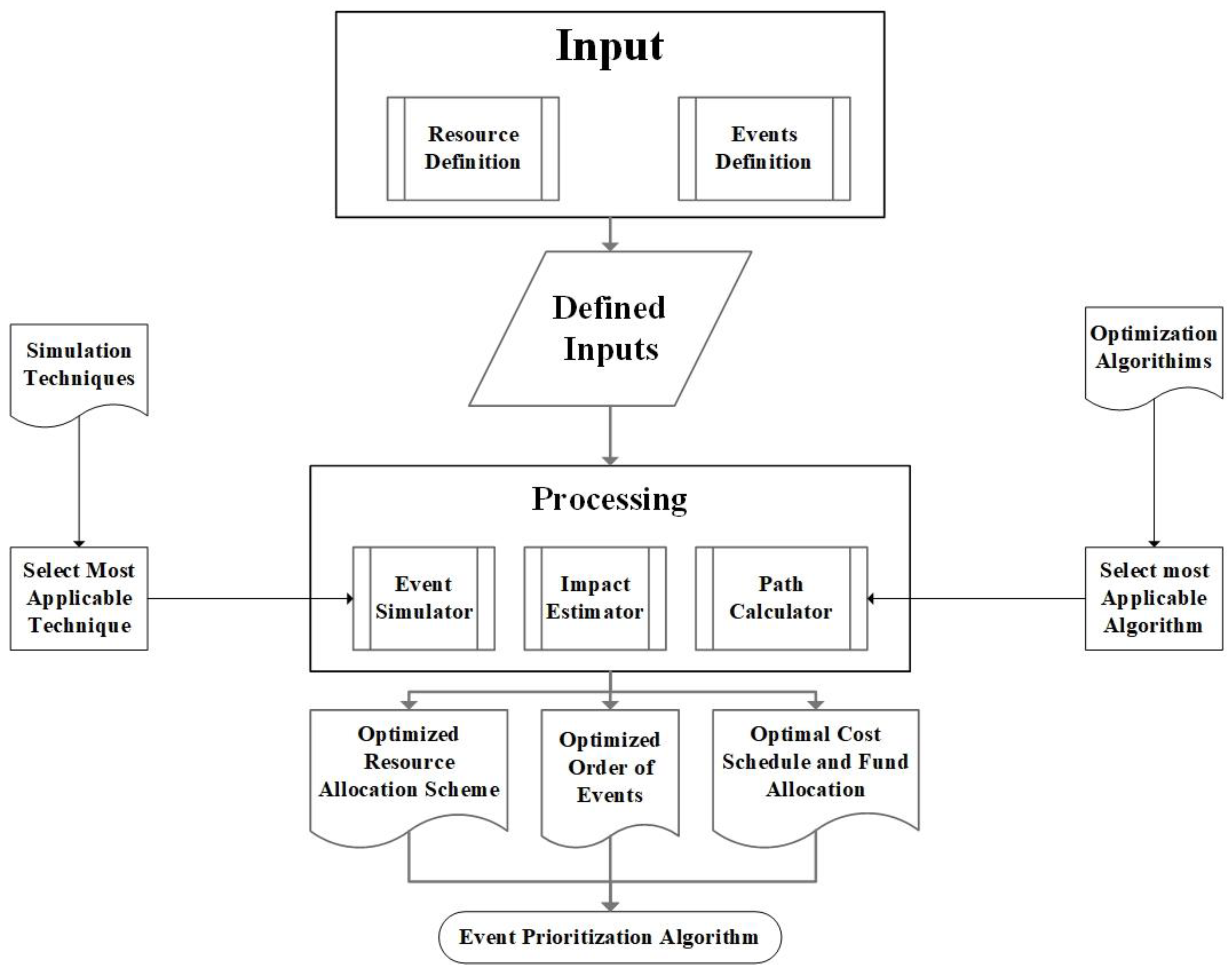
2.2. Inputs

To operate the Lazy Serpent Algorithm, a set of inputs is required to set up the three-dimensional space. Primarily, the events are distributed based on the three axes of importance specified by the user, with their specific range preferably 0 to 10. The inputs are classified on three levels: events, resources, and boundaries. The events in this specific case are discovered leaks and their respective information, as they are required by the algorithm. Resource input, also referred to as serpent input, indicates the number of available resources with their respective specific algorithm information. In the particular example given, it refers to the number of available repair teams. The third type of input is boundaries; however, boundaries are not a necessity for the operation of the lazy serpent. Thus, the algorithm can run without any constraints to find the optimal solution, regardless of the time or the resources required. However, constraints can be added to maximize or minimize the particular aspect the user wishes to tackle. For instance, a time constraint can be added to let the algorithm maximize the number of repairs in the specified limit.

2.2.1. Event Input

An event is simply an occurrence that has a certain state at the time it takes place. Thus, an event within the Lazy Serpent Algorithm is assumed to have an initial condition on all three axes of assessment (x₀, y₀, and z₀), in addition to the change of condition functions in each axis (f(x), f(y), and f(z)). The change equations are assumed to be a function of the same unit of time. In addition to the initial condition and the expected change in the condition through time, an event will have two other parameters, t_n and c_n, that identify the time expense and the financial expense. The parameter t_n indicates the amount of time needed for the complete disposal of the event and c_n indicates the total cost needed to handle the event completely. Therefore, an event A can be represented as A (x₀, y₀, z₀, f(x), f(y), f(z), t_n, c_n). The definition is further described in Equation (1), where the initial condition is part of the motion equations f(x), f(y), and f(z). The equations are composed of the initial condition x₀, y₀, and z₀, along with their relative variation through time g(t).

$$A=\{\begin{array}{l}f\left(x\right)=x_c+g_x\left(t\right)\\ f\left(y\right)=y_0+g_y\left(t\right)\\ f\left(z\right)=z_0+g_z\left(t\right)\end{array},t_n,c_n$$

(1)

For example, let us assume an event A with initial conditions (6,8,4) and a change in time g (−0.1t, −0.4t, 0) and a t_n of 8 days and a c_n of 100,000 dollars. Therefore, f(x), f(y), and f(z) would be (6–0.1t, 8–0.4t, 4). In case we want to determine the condition after four days of the initial investigation, we replace t with 4 and the results would be (6–0.1(4) = 5.6, 8–0.4(4) = 6.4, 4) and A₄ would be (5.6, 6.4, 4). Throughout the development of this algorithm, multiple conditions were identified that require the existence of multiple types of events to deal appropriately with each type of real-life event. The identified event types are enlisted as follows:

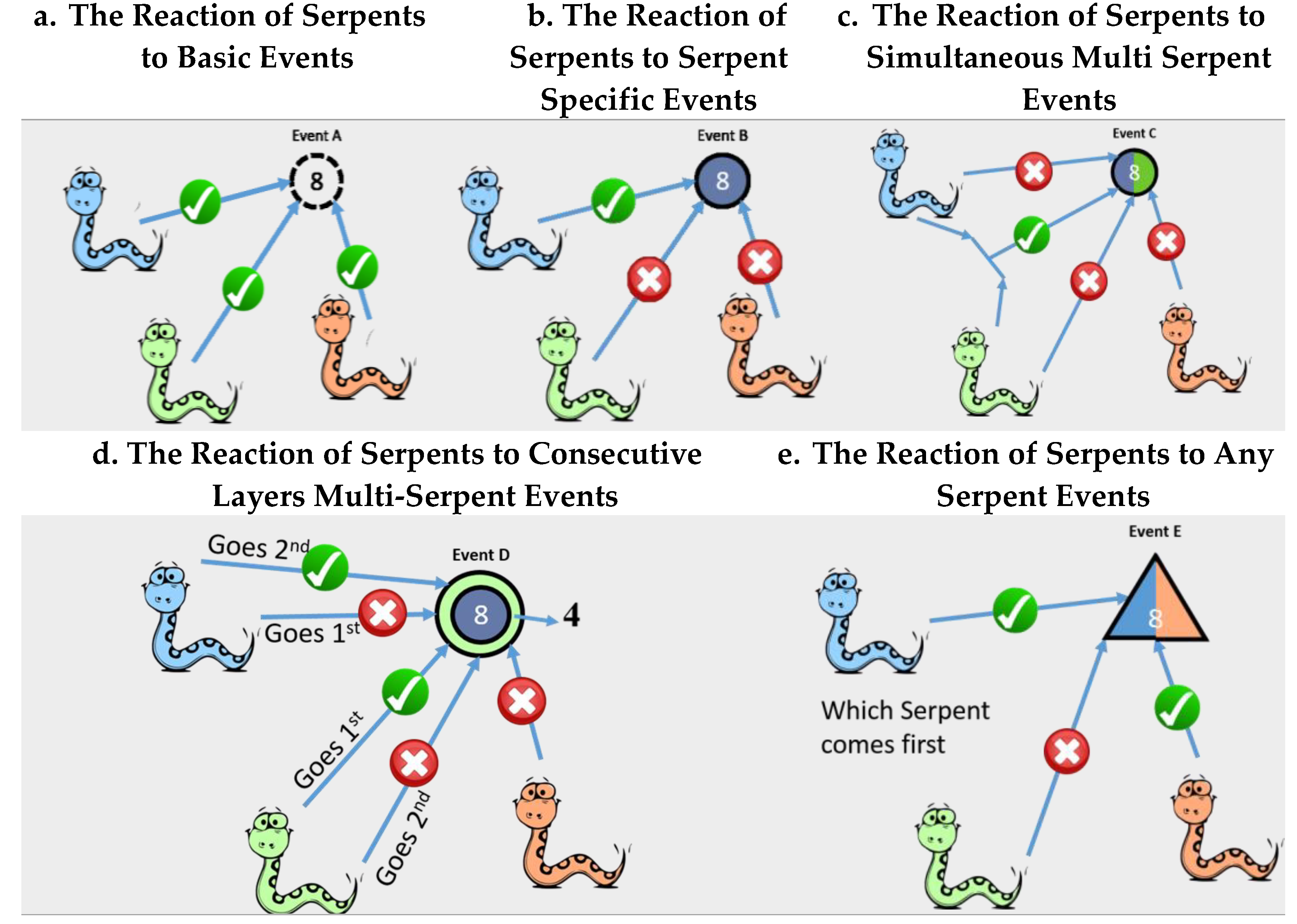
Basic Events (B)

The first event type is the basic event. A basic event is an event that has no specific nature or a specific approach, such as delivering a simple item or refilling a gas tank. Regarding leaks, it can be iterated as a simple leak that any available team can easily deal with it. Thus, a basic event would have no specific color and can be handled by any resource, as illustrated in Figure 3a. The drawing illustrated in Figure 3a shows that the basic Event A could be eaten by any of the three serpents based on a first-come-first-served approach. A basic event is represented as a colorless circle with a dotted circumference. The value eight located within event A represents the weight t_n that presents the time required to complete event A. Equation (2) presents the mathematical and logical presentation of basic events. For devouring to occur (e.g., event handling or leak repair), the event must be at the shortest distance from any serpent and that serpent must be idle. If the two conditions are met, the event begins to be devoured, and thus, in real life, the leak repair begins.

$$(d=min{\displaystyle \bigwedge }serpent=idle)\Rightarrow devour=true$$

(2)

Serpent Specific Events (SS)

The second event type is one that can be solved by only one type of resource. In this algorithm, they are dubbed as “Serpent Specific Events” and are represented by a specific color. Thus, only the matching serpent can handle this event and any other type of serpent would merely ignore it. The illustration in Figure 3b displays an event B colored in blue. Thus, the orange and green serpents are unable to react to event B and only the blue serpent can react to event B and complete it, whereas the remaining events stay idle even if they are available. A specific event is represented as a full circle filled with the color of the necessary type of serpents, along with the time weight t₀. Mathematically, serpent specific events can be illustrated using Equation (3). The equation shows that to have an event interaction between serpent and event, three conditions must be met. The distance conditions and the idle condition are the same from the previous section. The new condition for this type of event is color. The color of the event (color_e) and the color of the serpent (color_s) must match precisely to start the interaction.

$$\left(d=min{\displaystyle \bigwedge }serpent=idle{\displaystyle \bigwedge }colo{r}_e=colo{r}_s\right)\Rightarrow devour=true$$

(3)

Multi-Serpent Events (MS)

In real life, not all events or actions require one resource or team to be completed. As a result, multi-serpent events are developed. Multi-serpent events are events that require more than one resource (serpent) to complete and they are divided into two types:

(a)

Simultaneous: a simultaneous event is an event that requires the existence of two specific resources or more at the same time to be completed. Once commenced, all resources will suffer the same delay (t_n) required for the event, but the cost of the event (c_n) will be one regardless of the number of resources used. Further costs as the operational costs of each serpent are referred to as energy consumption; this concept will be explored later. Figure 3c displays how serpents react in the presence of a simultaneous event. Event C is not tackled when only one of the blue or green serpent is available; only when when both are available at the same time, event C is tackled and completed. A simultaneous event is drawn as a circle that is equally divided by the colors representing the required serpents along with the amount of the required time t₀.

On the level of mathematical representation, simultaneous multi-serpent events (SMSE) can be represented as a decision tree with three main decision criteria that must coexist at the same time. Each criterion has two primary objectives to be validated for it to be true. When all three criteria are valid, then the execution can be carried out. Equation (4) illustrates this idea by highlighting the three required conditions to carry out the assessment leading to decision making. The first criterion is the distance, where the two serpents are checked for their proximity from the event. The second is idleness and the last criterion is color matching.

$$\left(d_1=min{\displaystyle \bigwedge }{d}_2=min{\displaystyle \bigwedge }{s}_1=min{\displaystyle \bigwedge }{s}_2=idle{\displaystyle \bigwedge }c{s}_1+c{s}_2=c{e}_1+c{e}_2\right)\Rightarrow devour=true$$

(4)

(b)

Consecutive-Layers: Although prioritization algorithms do not normally deal with events with interdependencies, a certain type of event was noted with certain interdependencies that require being tweaked into the Lazy Serpent Algorithm. Consecutive-layers events are those that require more than one resource to be completed. The required resources must be available in a certain order. Therefore, consecutive-layers events are considered layered events that change their color after a serpent completes a layer to become another task that requires another resource. Figure 3d illustrates this concept by displaying event D that has a green outer layer and a blue sublayer. Event D will be treated as a green event until a green serpent (resource) is available to complete it. When completed, event D becomes a blue event and waits for an available blue serpent to be finalized. The blue serpent cannot tackle event D before the green serpent. Only after the green serpent is done can the blue serpent tackle event D. In terms of cost, a consecutive-layers event will not be charged until completion, i.e., until all layers are resolved. In this figure, the first layer requires four days to be performed, after which the event will become a blue event and require eight days to be finalized. On the level of coding and mathematical representation, consecutive-layers events are considered serpent-specific events based on their initial layer, as in Equation (3). However, after the primary interaction is completed, the devour command will trigger another command as in Equation (5), which is the transform command. The command transforms the event into another event after the serpent-event interaction. The equation displays the transformation of an event A_i from its first layer (A_i1) to its second layer (A_i2).

$$devour=true\Rightarrow transform\left(A_{i1}to{A}_{i2}\right)$$

(5)

Any-Serpent Events (AS)

Another type of event in the field is characterized as those that can be performed by a specific pool of resources. Thus, the difference between a basic event and an any-serpent event is that any existing resource can handle basic events, whereas any-serpent events are handled by any serpent from a predefined group of resources. Thus, as in Figure 3e, an any-serpent event is displayed as an equilateral triangle that is colored equally by the serpents (resources) capable of handling it. The figure shows event E is colored half orange and half blue, which means only the blue and the orange serpents can deal with event E. As a result, whichever of the two serpents is available first handles this task and has to spend the amount of time t_n, which is 8 days in the case of Figure 3e, that is required for completion. At that time, the serpent is categorized as digesting (unavailable resource), which means busy and unable to move or leave the location of event E.

Regarding mathematical representation, any-serpent events are similar to serpent specific events except for the matching condition where the closest serpent must belong to a pool of colors. As in Equation (6), the serpent is first checked for proximity, then availability and idleness, and finally if it belongs to a predefined set of colors. Equations 1 through 6 are provided in a pseudocode format in Appendix A.

$$\left(d=min{\displaystyle \bigwedge }serpent=idle{\displaystyle \bigwedge }colo{r}_s\in \left\{c_{e1},c_{e2}\right\}\right)\Rightarrow devour=true$$

(6)

2.2.2. Resource Input (Serpent Definition)

All serpents are governed by one single motion or action type called behavior and each serpent is then defined based on color and consumption as the two main variables. Regarding color, each serpent can have only one color, which represents the type of action the resource (serpent) could perform. However, consumption signifies the number of energy resources consumed per time (t_n) by the resource. During the time required by the resource t_n, the serpent is unable to move and is referred to by the term “digesting” (occupied) and stays at the location of the event until the process is complete. Beyond the completion of an event, the serpents will react according to a predefined behavior that governs the behavior beyond the task completion. The movement of the serpents by default is considered to be teleportation, where serpents move immediately to the nearest serpent. In future iterations of the algorithm, travel time could be included for better estimates.

The overall behavior defines the way the serpent behaves after devouring an egg (completing an event) and these reactions are divided into two main categories:

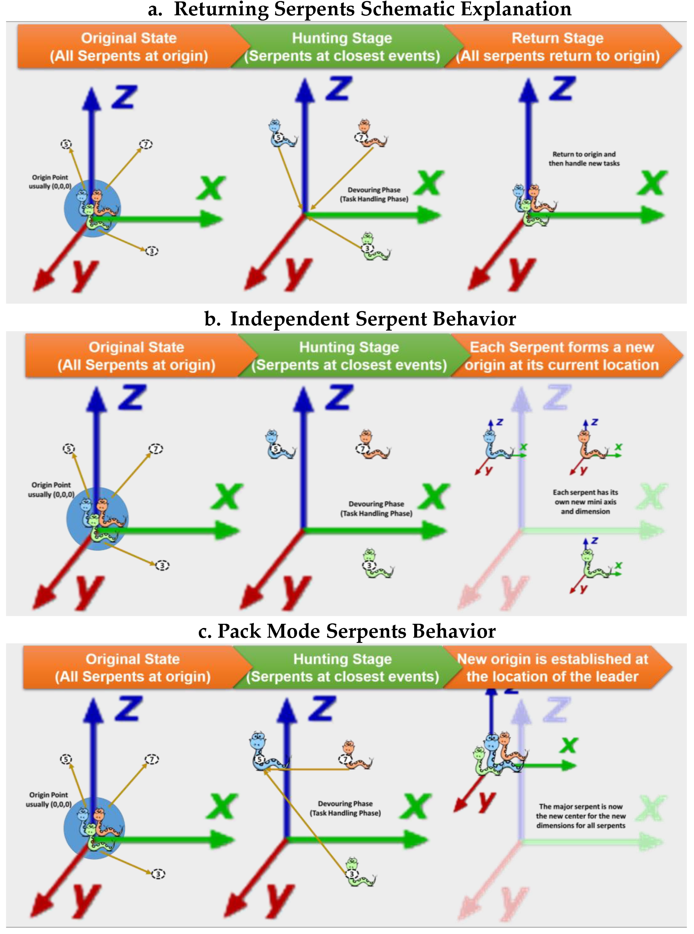
• Returning behavior assumes that all serpents will return to their headquarters, i.e., the point of origin specified by the user, which is default set at (0, 0, 0). Therefore, whenever a serpent (resource) finishes a task, the serpent will return to the origin point to select the next best event to tackle. Figure 4a displays this behavior as all serpents first set out to their targets and, after completing each task, the serpents shall return to the point of origin. Since the green serpent had the event with the lowest time consumption, it returns to the origin first and it immediately sets on to go to a new target if it exists, whereas the orange serpent would be the last to return to the origin point due to having its event requiring the most time.
• Establishing behavior—In practice, not all resources return to their starting point once they finish the task they are assigned. Rather, the resource would search for the problem nearest to its location to tackle it. Thus, the concept of establishing serpents or establishing behavior was developed to simulate the reality on the field. Establishing serpents can establish new origins as they are on their paths to determine the next best solution. Establishing serpents are divided into two main categories, independent and pack mode, which are defined as follows:

  (a)

  Independent—In this category, it is assumed that each resource selects the location of the finished task and establishes its respective location as a new point of origin. Immediately after setting the new point of origin, the serpent moves to select the event location closest to the newly established origin and solves it. After solving the second event, the serpent establishes the new location as a new origin point and this process goes on. Figure 4b illustrates the approach with more clarity. As highlighted, all serpents start at the origin point (0, 0, 0) and then move towards their targets. Later, after completing their tasks, each serpent has its origin point and it selects its next target accordingly.

  (b)

  Pack Mode—In some situations, a moving resource will be referenced as a strategic point or a moving command center that other units have to return to when they are done. Thus, a pack mode behavior requires the central resource to be selected and identified. The chief resource becomes the origin point as it moves and all other serpents have to return to the current location of the chief serpent (central resource) before going onto their next target. Figure 4c displays this behavior by showing the chief blue serpent at the origin point before each serpent embarks on its task. After completion, all serpents return to the blue serpent’s current location before heading off to their new tasks.

2.2.3. Boundaries

Boundaries are the third factor in setting the lazy serpent field. Although boundaries are not a must, they are critical to the decision-making process as they represent the constraints that the decision-maker, e.g., municipalities and project managers, have at hand. The primary two constraints for the Lazy Serpent Algorithm are time and energy (cost). Time as a constraint represents the total amount of time consumed by the overall algorithm and energy represents the cost consumed by the project. However, energy is a general term, too, as money might not be the only resource of concern that is consumed by the project.

Based on what is discussed above, the governing factor is the relationship between benefit and cost. This relationship is predetermined based on the type of problem. For the problem of leak repair, all leaks are assumed to be deteriorating, and therefore the faster they are repaired, the better it is for saving precious water resources and minimizing their impending damage. Based on this assumption, the benefit of an event is the collected value of its current point. For example, an event H is repaired when it reaches the point (4, 7, 6) in the 3D space. Therefore, its benefit is b_tH = 4 + 7 + 6 = 17. Further illustration is provided by Equation (7), where the benefit at termination b_tH is equal to the summation of the end of repaired-event coordinates in the 3D space. When an event is being resolved it ceases to move, thus the assumption would be that an event does not get worse during repair, and accordingly, it remains at the same point in the 3D system.

$$b_{ti}=x_{ti}+y_{ti}+z_{ti}$$

(7)

However, the cost is the summation between the cost needed (c_ni) by the event and the resource operational costs calculated by multiplying the time needed for repair (t_ni) by the cost rate of the resource (r_cs). The illustration of this concept can be found in Equation (8), where each event has its own overall cost.

$$C_{Oi}=c_{ni}+\left(t_{ni}\times r_{cs}\right)$$

(8)

Based on the two event equations, the total benefit of a solution is the summation of all the benefit values of all the events that comprise the selected solution, as displayed in Equation (9). The equation shows the approach to determine the total benefit (B) of a solution by calculating the respective benefits. Letter n refers to the total number of events within the solution.

$$B={\displaystyle \sum }_{i=1}^n{b}_{ti}$$

(9)

Similarly, the total cost of a solution is the summation of the costs of all the events comprising this solution, as in Equation (10), where the total cost (C) is the sum of all the events in the solution whose number is n. Moreover, the benefit-to-cost ratio is the division of B from Equation (9) over C from Equation (10).

$$C={\displaystyle \sum }_{i=1}^n{C}_{Oi}$$

(10)

Thus, the following approaches are identified:

• Free/Unbound—The primary assumption in the unbound setup is that energy (money) and time are abundant and can be spent openly. The field of the algorithm has no constraints and thus the algorithm runs until all events are completed and solved. Furthermore, the algorithm tries to figure out the best path with the lowest time and energy consumption. Equation (11) illustrates the optimization goal of this mode, which is to find the maximum benefit-to-cost ratio for all possible schedules.

  $$max\left\{\frac{B}{C}\right\}$$

  (11)
• Time-Bound—In this approach, it is mainly assumed that energy (fund) is abundant but time is scarce. Thus, a time limit (T) exists, forcing the algorithm to stop after the running time (t_run) reaches the time limit (T). Thus, the main aim of the algorithm is to maximize the benefit-to-cost ratio within the time limit regardless of cost. In Equation (12), the previously mentioned conditions and goals can be summarized by an optimization equation.

  $$max\{\frac{B}{C}/t_{run}\le T\}$$

  (12)
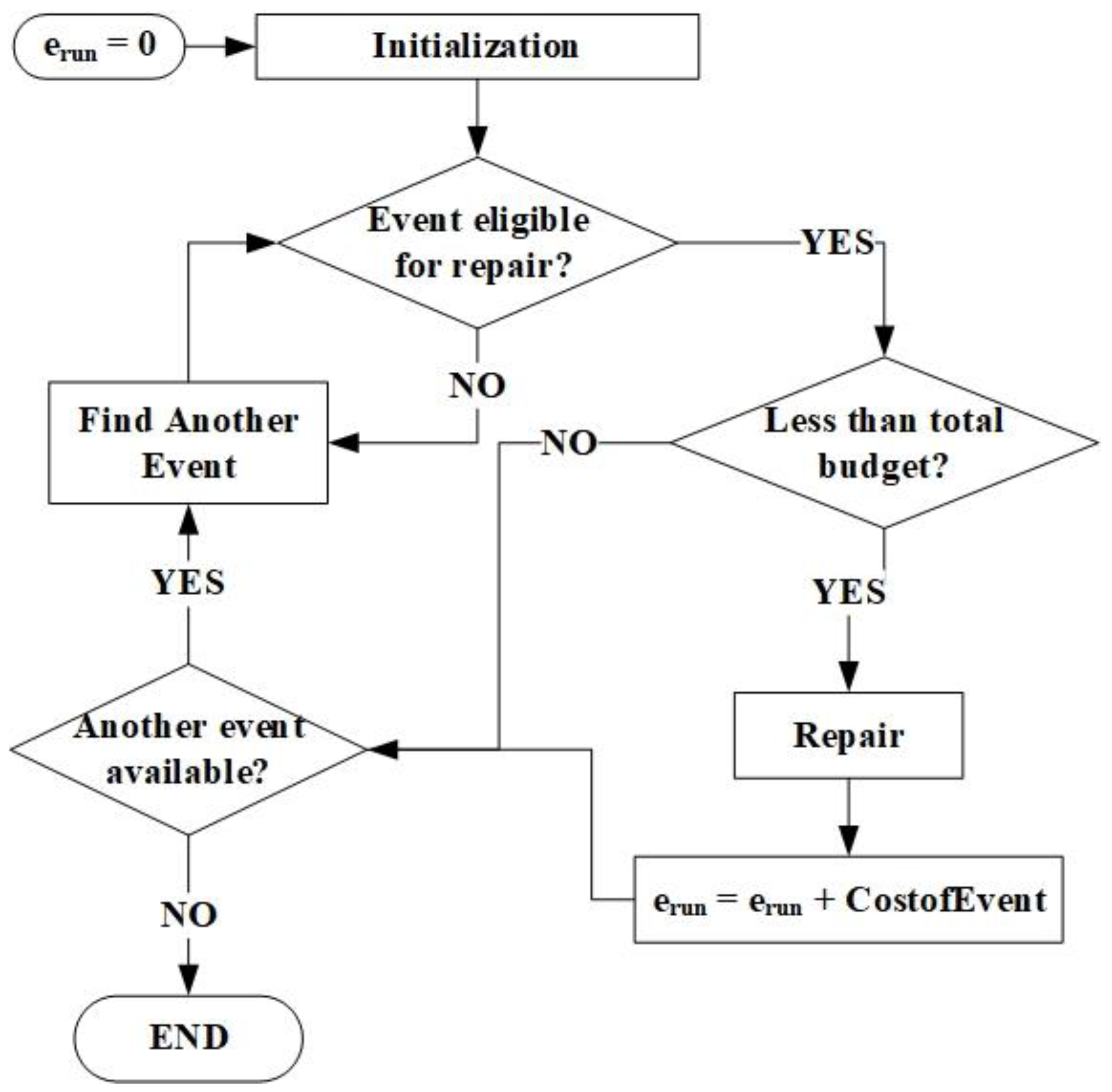
• Energy Bound—The exact reverse of a time boundary is an energy boundary (E). The main assumption is that time is abundant and holds no constraints whereas funds are scarce and must be efficiently allocated. Therefore, the algorithm tends to maximize the number of tasks performed for a specific amount of energy (funds). Equation (13) displays the approach of maximizing the benefit-to-cost ratio for a maximum allotted energy or fund (E) that the solution expenditure or cost (e_run) must never exceed.

  $$max\{\frac{B}{C}/e_{run}\le E\}$$

  (13)
• Dual Boundaries—The main condition under this boundary is that both energy and time are scarce. Thus, the algorithm tends to maximize the number of tasks performed within the limits of time and energy, as displayed in Equation (14).

  $$max\{\frac{B}{C}/t_{run}\le T,e_{run}\le E\}$$

  (14)

The optimization equations above can be summarized in Equation (15). The main objective is to maximize the benefit of the incurred expenses, taking into consideration a specific timeline and overall budget. One or both constraints can be removed depending on the user’s needs.

$$\begin{array}{c}max\frac{B}{C}\\ s.t.:\\ t_{run}\le T\\ e_{run}\le E\end{array}$$

(15)

Another field setup is the threshold. A threshold in the Lazy Serpent Algorithm is a set of values on each plane that represents a borderline that the user, e.g., municipalities, prefers not to cross at all costs. A threshold is made of three planes with specific values along with the intersection with the origin planes. Not all axes need to have thresholds; it is possible to have all or none. A threshold represents the worst condition from the eyes of the user; thus, if an event crosses a threshold, the event has crossed into an undesirable condition. Once an event or multiple events cross the threshold, the Lazy Serpent Algorithm notifies the user that there might be a need to increase the number of resources to prevent further events from crossing the threshold.

2.2.4. Proposed Solution: Inverse Pyramid

To solve the lazy serpent problem, a greedy solution is proposed, where the serpent tries to maximize the number of events consumed. The solution imagines the 3D space events in a planar space that consists of the points of distance calculated previously. The first event to be selected is the event with the lowest distance since it fits the budget and time constraints, as shown in Figure 5 and Figure 6. Figure 5 shows that the algorithm starts with an initially assigned population of all the events under analysis. Whenever an event is contained, a new plane is created without the handled event. The selected mode of analysis is then performed on the new plane and the cycle is repeated until all constraints are met. Hence, the name “inverted pyramid” solution, where the solution starts with the complete population at first and then proceeds to develop new populations that are smaller than the earlier populations due to the eliminations process. The selected event is then removed from the plane and is replaced with infinity, and a new plane is formed with an updated time that adds the repair time taken to repair the event. The solution would continue to run and eliminate solutions until it hits either the budget or the time constraint.

Figure 6 further illustrates the form of updating the equations of the solution. Initially, e_run is equal to zero and, after initialization, the first event is selected. If the event meets the repair criteria, then it is repaired and its cost is added to e_run, which continues to update itself based on this criterion until it meets the budget constraint or finds no more available events for repair. Similarly, time is updated with the same fashion using the variable t_run, which keeps on selecting and updating events simultaneously with e_run. If one event does not meet the criteria of both equations, then the event is dropped, and the code would try to find another event that fits the criteria.

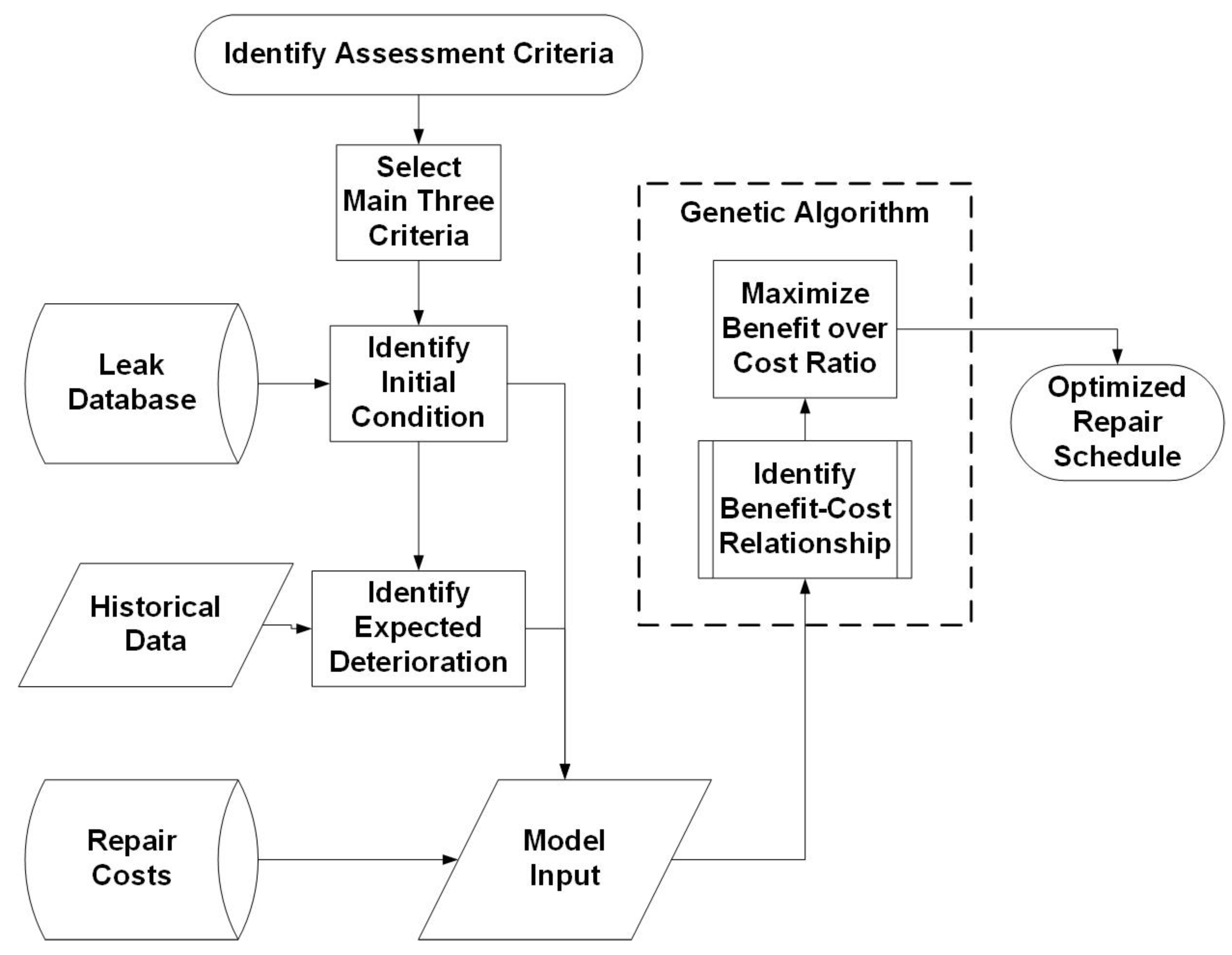
2.3. Genetic Algorithm Comparative Model

The genetic algorithm is one of the most widely used evolutionary algorithms that proved its efficiency in handling multiple conflicting objectives directly and simultaneously [22,23,24]. The first stage involves creating a random population of solutions where the solutions are represented in the form of a string called “chromosomes” or “individuals.” In genetic algorithms, a solution to a problem is an “individual” and the group of solutions in each stage is a “population.” In the second stage, a new population of individuals is created and called “generation.” A fitness function is used to assess different chromosomes. There may be more than one fitness function in the case of multiobjective optimization. The fitness of each chromosome is determined by evaluating it against the objective function. The third stage encompasses the selection of chromosomes. The selection process determines which chromosomes will mate to form new chromosomes. There are different types of chromosomes selection strategies: roulette wheel selection, rank selection, steady-state selection, elitism, Boltzmann selection, and tournament selection. The fourth stage is to perform a crossover. Crossover is a very important process to generate an offspring between two chromosomes or individuals. There are different types of crossover: single point, two point, and uniform. The fifth stage is to perform mutation. The mutation gene is chosen randomly. The process of mutation occurs by looping through all genes of individuals and if a gene is selected for mutation, the gene will be changed by a small value or it will be replaced by a new value. The mutation is done to ensure that individuals are not the same and to ensure genetic diversity within the population. The mutation is also performed to avoid stagnation around local minima. The mutation rate is usually less than 0.1. Finally, a population is generated in each generation, and the above processes continue for a certain number of iterations. The chromosomes in the final iteration are the solutions.

To compare the Lazy Serpent Algorithm to other algorithms, a genetic algorithm model was developed. The model aimed to utilize an approach similar to that of the lazy serpent such that it uses a 3D environment with motion variables such as costs and time. The purpose of the genetic algorithm model was to identify the schedule with the best benefit-to-cost ratio. For the development of this model, the evolver tool by Palisade was used with an Excel sheet. The following settings were used for model development: (1) crossover rate = 0.8, (2) mutation rate = 0.05, and (3) tournament selection was utilized as the parent selection method.

Figure 7 displays the methodology used to develop the genetic algorithm model for prioritization. The first stage was to identify the main assessment criteria via literature review and common practices. The second stage was to select the three main criteria for assessing each repair event. The next step was to identify the initial condition of each leak and then, based on historical data, to predict the decay and deterioration equations of the leak as a function of time. Furthermore, leak costs and repair costs were identified to finalize the process that defined the inputs. Before launching the genetic algorithm model, the benefit–cost relationship amidst the defined criteria should be identified to be maximized. For this model, a fundamental relationship between the cost and the factors was developed and is illustrated in Equation (16); the equation assuming that a leak is repaired in the best state and what remains is savings and benefits. The factors L, M, and N represent the adjustment factors for a specific measure and are used to identify the impact of each factor on the benefit–cost relationship [25,26].

$$\frac{B}{C}=\frac{L{x}_i+M{y}_i+N{z}_i}{c_i}$$

(16)

where:

-

B/C = benefit-to-cost ratio;

-

x, y, and z = main assessment factors;

-

L, M, and N = factor adjustment weights;

-

I = represents the number of the event under study;

-

c_i = cost of repairing the event i.

The optimization goal can be summarized in Equation (17). The goal is to maximize the total value of the benefit-to-cost ratio such that the total cost (e_run) is less than the budget (E) and the total time required to finish the tasks (t_run) is less than the allocated time (t). The variable e_run is the total cost spent on the completed repairs and t_run is the total time used to complete the repairs.

$$max{\displaystyle \sum }{\frac{B}{C}}_T|\mathrm{Such}\mathrm{that}\{\begin{array}{c}{e}_{run}\le Budget\left(E\right)\\ t_{run}\le TimeScheduled\left(T\right)\end{array}$$

(17)

3. Results and Discussion

In this section, the models for schedule optimization are implemented in an example and their results are presented and compared. First, the implementation and results of the GA model are presented and the multiple aspects and results of implementing the Lazy Serpent Algorithm are discussed. The aim is to find the optimal order for repairs that maximizes the value of the money spent.

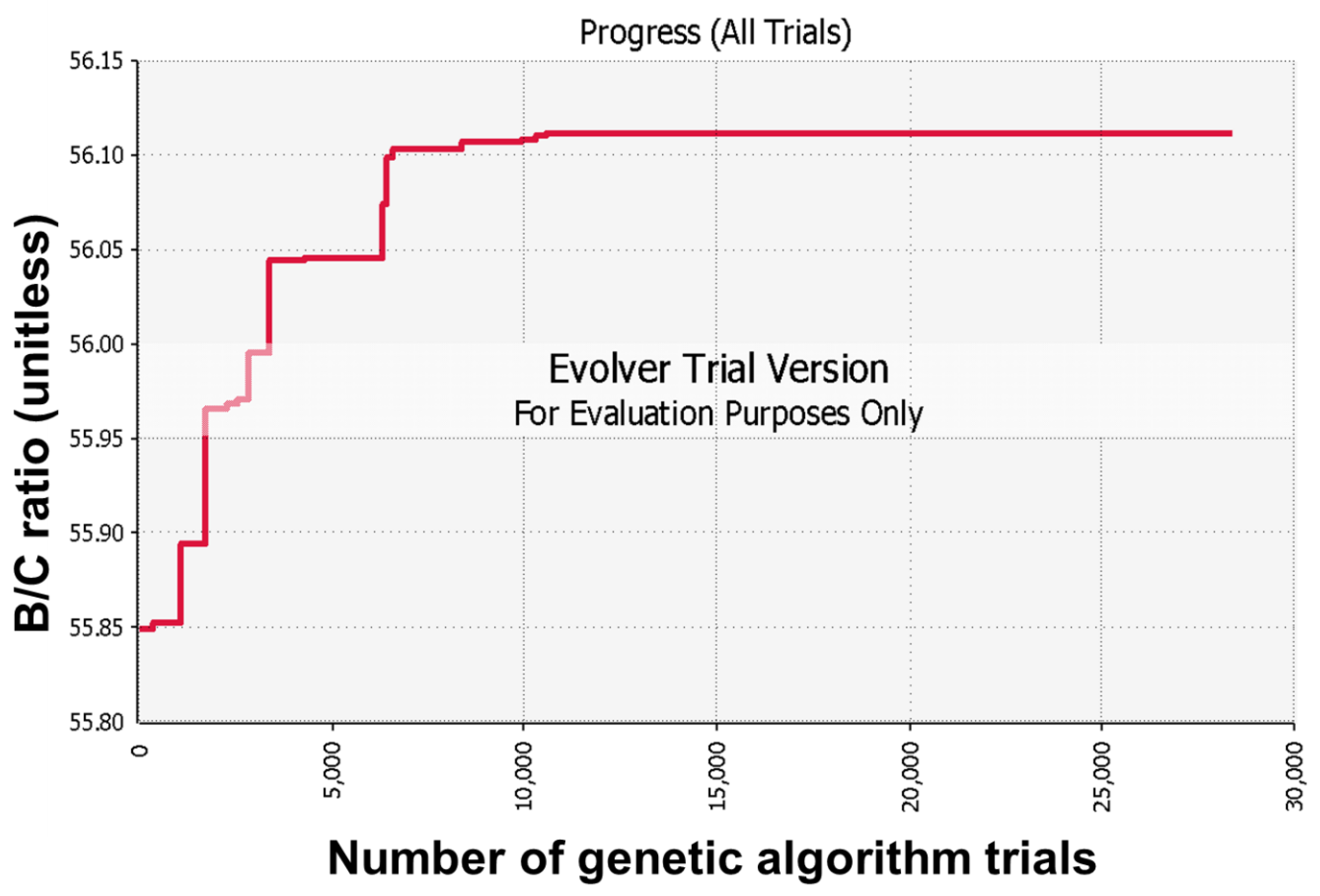
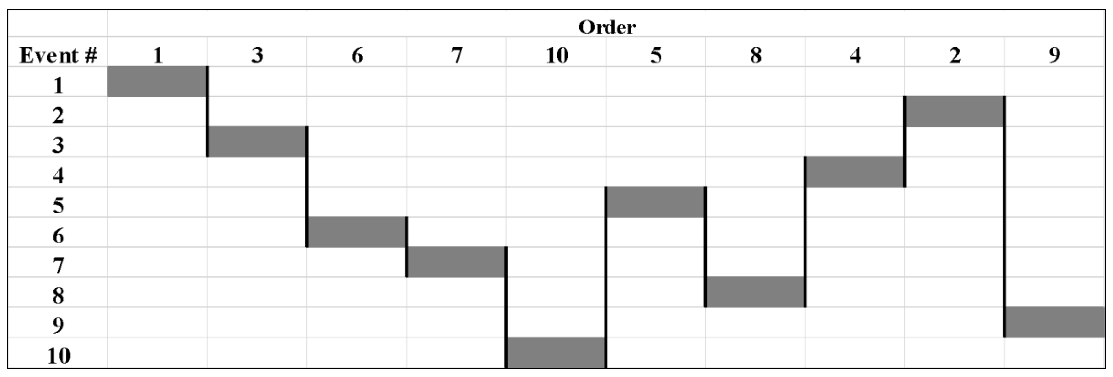
3.1. Genetic Algorithm Model Implementation and Results

A fictitious sample was prepared to test the developed genetic algorithm prioritization model. The sample consists of 10 main events that are decaying linearly and have three main assessment criteria extracted from literature (i.e., condition, criticality, and consequence of failure (COF)). The values of the assessed factors were generated randomly, as well as their repair periods and repair costs.

Table 1. Genetic algorithm input and output Excel sheet (COF, consequence of failure; B/C, benefit-to-cost ratio).

ID	Order	Condition	Criticality	COF	Repair Period (Days)	Repair Cost ($)	Condition at Repair	Criticality	COF	B/C
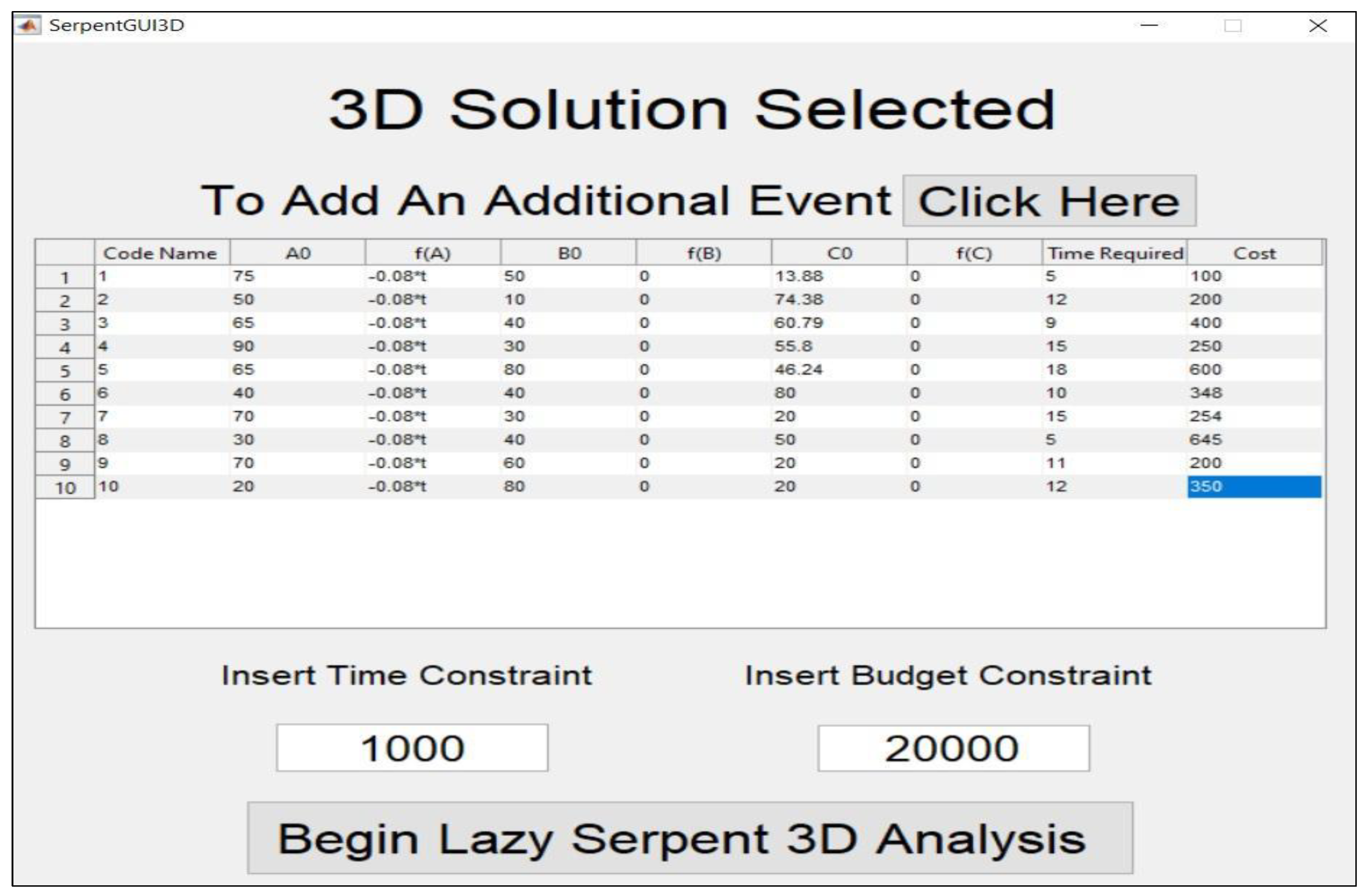
1	1	75	50	13.88	5	100	75	50	13.88	13.89
2	3	50	10	74.38	12	200	48.72	10	74.38	6.65
3	6	65	40	60.79	9	400	61.56	40	60.79	4.06
4	7	90	30	55.8	15	250	85.84	30	55.8	6.87
5	10	65	80	46.24	18	600	57.48	80	46.24	3.06
6	5	40	40	80	10	348	37.36	40	80	4.52
7	8	70	30	20	15	254	64.64	30	20	4.51
8	4	30	40	50	5	645	27.76	40	50	1.83
9	2	70	60	20	11	200	69.6	60	20	7.48
10	9	20	80	20	12	350	13.44	80	20	3.24
B/CSum = 56.11

displays the overall input for constructing the genetic algorithm model. The variable the algorithm tries to optimize is B/C. Furthermore, time requirements and costs are stated for each required repair. For this example, the algorithm is given the time to run all possible scenarios and select the best alternative. Additionally, the algorithm has no constraints regarding time or budget.

The algorithm requires 68 min to arrive at the optimal solution after testing all the possible scenarios. The total number of trials is 28,385, of which 15,456 trials are valid. Figure 8 displays the improvement path of the solution throughout trials, from the initial solution of 55.85 to 56.11 in benefit-to-cost ratio.

To establish an equal ground for comparison with the GA model, only one serpent was utilized. Since only one serpent was utilized, all events can be considered all-serpent events. Based on that, the optimized schedule and repair order for the maximized benefit-to-cost ratio is shown in Figure 9, where the optimal order of the previous example is displayed as the following order of events: 1, 3, 6, 7, 10, 5, 8, 4, 2, and 9.

3.2. Lazy Serpent Model Comparative Results

The Lazy Serpent Algorithm is compared to the genetic algorithm using the same sample data in the previous section. Multiple instances of the Lazy Serpent Algorithm are run with different selection criteria definitions. The aim is to explore the aspects of the lazy serpent and see the extent of its power as a prioritization algorithm. Figure 10 displays the interface of the lazy serpent software developed using MATLAB which is produced by MathWorks in Massachusetts, USA. The interface consists of multiple parameters, first the codename where the user inputs the name of the event to be scheduled. The codename can be numeric or alphabetic or a mixture of both. The next set of parameters is A0, B0, and C0, which represent the initial condition upon the discovery of the event at the point of assessment. The second set of variables is f(A), f(B), and f(C), which represent the change in the condition of each event. In this example, all events deteriorate in one plane and the deterioration function is −0.08 *t. Moreover, two variables to identify the required time and cost for each event are added under the tabs Time Required and Cost. Finally, the constraints are added via the Time Constraint and Budget Constraint. The Lazy Serpent Algorithm is run with three different selection criteria: (1) the basic Lazy Serpent Algorithm, which consists of selecting the worst condition event each time and eliminating it; (2) the inverse lazy serpent, which selects the best event each time; and (3) the selective lazy serpent, which aims at selecting the most deteriorating event through projection. If two events have equal deterioration factors, the one with the lowest price will be selected; if the price is the same, then the algorithm will move to select the one with the minimum required time. If all factors of selection are equal, an event will be chosen randomly.

3.2.1. The Basic Lazy Serpent Results

The basic lazy serpent selects the closest event to the origin. Then, it selects the most deteriorating events first and goes upwards until it meets a constraint, or it finishes all the available events. Figure 11 shows the results presented by the basic lazy serpent with deterioration preference as follows: starting with event 8, followed by event 7, event 10, event 2, event 1, event 9, event 3, event 6, event 4, and event 5. The algorithm requires 6 s to come up with this solution, as the lazy serpent does not search for all possible outcomes like the genetic algorithm. On the contrary, it goes immediately towards an expected solution. The quality of the solution is measured by the final benefit-to-cost ratio calculated by assuming the remaining three-dimensional values at the point of repair initiation as benefits. The final benefit-to-cost ratio of the proposed solution is calculated to be at 55.81 or 5.581, which is slightly less than that of the first-in-first-out approach.

3.2.2. The Inverse Lazy Serpent Results

The inverse lazy serpent relies on selecting the farthest events from the origin. In other words, it selects the best events available. The inverse lazy serpent presents a different order from the basic lazy serpent. The schedule starts with event 5, followed by events 4, 6, 3, 9, 1, 2, 10, 7, and event 8, as illustrated in Figure 12. The benefit-to-cost ratio measures the quality of the solution. The ratio is calculated to be 55.31 or 5.531 and the algorithm requires 6 s to arrive at the proposed solution.

3.2.3. The Selective Lazy Serpent Results

The selective lazy serpent has more advanced decision-making and selection criteria. The selective lazy serpent aims to select events with a higher deterioration rate than other events, thus it selects the most deteriorating event first. Furthermore, in case deterioration factors are equal between two events, the serpent moves ahead to select the one with the lowest price; if the price between two events is equal, the serpent moves to select the one with the lowest time requirements. Finally, if all the aspects are equal, the lazy serpent randomly selects an event from the pool. The results of the selective lazy serpent can be viewed in Figure 13. The proposed schedule starts with event 1, followed by event 9, event 2, event 4, event 7, event 6, event 10, event 3, event 5, and event 8. The time required for the development of this solution is 20 s and the benefit-to-cost ratio of the solution is calculated to be 56.19 or 5.619.

3.3. Comparative Analysis of Scheduling Results

All the scheduling results previously mentioned are summarized in

Table 2. Comparison of prioritization models (FIFO, first-in-first-out).

Algorithm/Approach	Inverse Lazy Serpent	Basic Lazy Serpent	FIFO	Genetic Algorithm	Selective Lazy Serpent
Results (B/C ratio)	5.531	5.581	5.585	5.611	5.619
Time Consumed	8 s	8 s	0	67 min	20 s

. Table 2 compares and analyzes the impact of each approach. The approaches and algorithms under study are (1) inverse lazy serpent, (2) basic lazy serpent, (3) first-in-first-out (FIFO), (4) genetic algorithm, and (5) selective lazy serpent. The initial benefit-to-cost value of the FIFO approach is calculated, and it is 5.585 value per dollar. Although the results are comparatively good, the FIFO approach cannot be relied on to construct a schedule regularly, as it is random and unpredictable, and thus its results can be good or bad with no consistency. The inverse lazy serpent gives the least benefit-to-cost ratio and therefore it can be concluded that leaving the worst for last can be a wrong approach and costlier than the remaining approaches. The basic lazy serpent has more acceptable results with a value of 5.581, which is close to the original 5.585 presented by the FIFO approach. Both the inverse lazy serpent and the basic lazy serpent require 8 s to give their results, which is considerably fast. The genetic algorithm presented the first improvement to the schedule with a benefit-to-cost ratio of 5.611, which is higher than those of the FIFO approach, the inverse lazy serpent, and the basic lazy serpent. The genetic algorithm requires 67 min to solve because the genetic algorithm tries to search throughout all the possibilities to arrive at a feasible solution. Finally, the selective lazy serpent gives a solution with the highest benefit-to-cost ratio with a value of 5.619 or 56.19. The selective lazy serpent requires 20 s to develop and present the schedule. The main reason for the selective lazy serpent is surpassing the genetic algorithm in terms of computational time is that the selective lazy serpent goes immediately towards building a solution, which contrasts with inspecting multiple options, as done by the genetic algorithm.

Statistical analysis is an important approach that demonstrated its capability in evaluating machine learning models [27] and metaheuristic optimization algorithms [28]. In this context, nonparametric testing is applied to evaluate the statistical significance levels of the optimization algorithms in prioritizing leak repairs. This is accomplished using Wilcoxon test, binomial sign test, and Mann–Whitney U test models at a significance level of 0.05 [29]. The statistical tests performed examine the null hypothesis ($H_0$), which implies that there is no significant difference between the optimization results. On the other contrary, the alternative hypothesis ($H_1$) implies that there is a significant difference between the classification results obtained from each pair of optimization algorithms. If the $p-value$ is less than the significance level, then the null hypothesis is rejected in favor of the alternative hypothesis. Nonetheless, if the $p-value$ is more than the significance level, then the null hypothesis is accepted.

Table 3. Statistical comparison between the optimization algorithms based on the Wilcoxon test.

Pair of Algorithms	Inverse Lazy Serpent	Basic Lazy Serpent	FIFO	Genetic Algorithm	Selective Lazy Serpent
Inverse Lazy Serpent	$H_0$($p-value$ = 1)	$H_1$($p-value$ = 2.7 × 10−3)	$H_1$ ($p-value$ = 2.7 × 10−3)	$H_1$ ($p-value$ = 7.69 × 10−3)	$H_1$ ($p-value$ = 2.7 × 10−3)
Basic Lazy Serpent	$H_1$($p-value$ = 2.7 × 10−3)	$H_0$ ($p-value$ = 1)	$H_1$ ($p-value$ = 2.7 × 10−3)	$H_1$ ($p-value$ = 7.69 × 10−3)	$H_1$ ($p-value$ = 2.7 × 10−3)
FIFO	$H_1$($p-value$ = 2.7 × 10−3)	$H_1$ ($p-value$ = 2.7 × 10−3)	$H_0$ ($p-value$ = 1)	$H_1$ ($p-value$ = 7.69 × 10−3)	$H_1$ ($p-value$ = 2.7 × 10−3)
Genetic Algorithm	$H_1$($p-value$ = 7.69 × 10−3)	$H_1$ ($p-value$ = 7.69 × 10−3)	$H_1$ ($p-value$ = 7.69 × 10−3)	$H_0$ ($p-value$ = 1)	$H_1$ ($p-value$ = 7.69 × 10−3)
Selective Lazy Serpent	$H_1$ ($p-value$ = 2.7 × 10−3)	$H_1$ ($p-value$ = 2.7 × 10−3)	$H_1$ ($p-value$ = 2.7 × 10−3)	$H_1$ ($p-value$ = 7.69 × 10−3)	$H_0$ ($p-value$ = 1)

,

Table 4. Statistical comparison between the optimization algorithms based on the binomial sign test.

Pair of Algorithms	Inverse Lazy Serpent	Basic Lazy Serpent	FIFO	Genetic Algorithm	Selective Lazy Serpent
Inverse Lazy Serpent	$H_0$ ($p-value$ = 1)	$H_1$ ($p-value$ = 0)	$H_1$ ($p-value$ = 0)	$H_1$ ($p-value$ = 0)	$H_1$ ($p-value$ = 0)
Basic Lazy Serpent	$H_1$ ($p-value$ = 0)	$H_0$ ($p-value$ = 1)	$H_1$ ($p-value$ = 0)	$H_1$ ($p-value$ = 0)	$H_1$ ($p-value$ = 0)
FIFO	$H_1$ ($p-value$ = 0)	$H_1$ ($p-value$ = 0)	$H_0$ ($p-value$ = 1)	$H_1$ ($p-value$ = 0)	$H_1$ ($p-value$ = 0)
Genetic Algorithm	$H_1$ ($p-value$ = 0)	$H_1$ ($p-value$ = 0)	$H_1$ ($p-value$ = 0)	$H_0$ ($p-value$ = 1)	$H_1$ ($p-value$ = 0)
Selective Lazy Serpent	$H_1$ ($p-value$ = 0)	$H_1$ ($p-value$ = 0)	$H_1$ ($p-value$ = 0)	$H_1$ ($p-value$ = 0)	$H_0$ ($p-value$ = 1)

and

Table 5. Statistical comparison between the optimization algorithms based on the Mann–Whitney U test.

Pair of Algorithms	Inverse Lazy Serpent	Basic Lazy Serpent	FIFO	Genetic Algorithm	Selective Lazy Serpent
Inverse Lazy Serpent	$H_0$ ($p-value$ = 1)	$H_1$ ($p-value$ = 4.66×10−5)	$H_1$ ($p-value$ = 4.66 × 10−5)	$H_1$ ($p-value$ = 1.61 × 10−4)	$H_1$ ($p-value$ = 4.66 × 10−5)
Basic Lazy Serpent	$H_1$ ($p-value$ = 4.66 × 10−5)	$H_0$ ($p-value$ = 1)	$H_1$ ($p-value$ = 4.66 × 10−5)	$H_1$ ($p-value$ = 1.61 × 10−4)	$H_1$ ($p-value$ = 4.66 × 10−5)
FIFO	$H_1$ ($p-value$ = 4.66 × 10−5)	$H_1$ ($p-value$ = 4.66 × 10−5)	$H_0$ ($p-value$ = 1)	$H_1$ ($p-value$ = 1.61 × 10−4)	$H_1$ ($p-value$ = 4.66 × 10−5)
Genetic Algorithm	$H_1$ ($p-value$ = 1.61 × 10−4)	$H_1$ ($p-value$ = 1.61 × 10−4)	$H_1$ ($p-value$ = 1.61 × 10−4)	$H_0$ ($p-value$ = 1)	$H_1$ ($p-value$ = 1.61 × 10−4)
Selective Lazy Serpent	$H_1$ ($p-value$ = 4.66 × 10−5)	$H_1$ ($p-value$ = 4.66 × 10−5)	$H_1$ ($p-value$ = 4.66 × 10−5)	$H_1$ ($p-value$ = 1.61 × 10−4)	$H_0$ ($p-value$ = 1)

report the $p-values$ of the optimization algorithms, capitalizing on the Wilcoxon, binomial sign, and Mann–Whitney U tests. As can be seen, the $p-values$ of the pairs (Selective Lazy Serpent, Inverse Lazy Serpent), (Selective Lazy Serpent, Basic Lazy Serpent), (Selective Lazy Serpent, FIFO), (Selective Lazy Serpent, Genetic Algorithm), and (Selective Lazy Serpent, Selective Lazy Serpent) for all the tests are less than 0.05. This implies that the selective Lazy Serpent Algorithm significantly outperformed other optimization algorithms in prioritizing leak repairs.

4. Conclusions

The Lazy Serpent Algorithm was inspired by the need to solve a combinatorial optimization problem with a variety of constraints. Accordingly, the user can replicate the model by imaging the optimization problem they are tackling in a dynamic three-dimensional environment that changes with time. They need to identify their resources first, the events they are tackling second, the changes through time third, and finally their constraints.

The Lazy Serpent Algorithm provides a reliable approach to the prioritization of goals that change over time. The approach provides quick results that can be adapted and updated regularly to suit incoming new data or to remove old and resolved data. When compared with the genetic algorithm, some selection criteria provided results that are close to the genetic algorithm’s result but with comparatively lower computational time. Additionally, one selection criterion provided a much better result within a much lower computational time as well. A further comparative analysis was conducted to investigate the statistical significance levels of the optimization algorithms. In this context, it was inferred that the selective Lazy Serpent Algorithm significantly outperformed other optimization algorithms in prioritizing leak repairs. This has been confirmedby the results obtained from the Wilcoxon, binomial sign, and Mann–Whitney U tests. This can provide municipalities with high improvements on the returns of their investments compared to the conventional approaches that are used.

Based on what preceded, it is safe to deduce that the lazy serpent can provide efficient and practical prioritization and scheduling for decision-makers in any field. Noting that the Lazy Serpent Algorithm outperformed the widely used genetic algorithm in terms of result quality and time, the lazy serpent still has great potential for improvement. The aforementioned results were also validated by a variety of statistical tests and assessments.

The Lazy Serpent Algorithm still has room for improvement by integrating other forms of event definition and selection criteria, for example, by utilizing probabilistic functions as simulation engines to define repair times more accurately. Another aspect of improvement to be studied is the integration with chaotic mechanisms. Surveying this option may help uncover better search modes for the serpents and therefore generate better results. Furthermore, the optimization model can be extended to encompass simulation of sustainability and environmental performance aspects.

References

- Davis, S. Priority Algorithms. Available online: http://cseweb.ucsd.edu/~sdavis/res_exam.pdf (accessed on 24 January 2017).
- Colorni, A.; Dorigo, M.; Maniezzo, V. A Genetic Algorithm to Solve the Timetable Problem; Politecnico di Milano: Milan, Italy, 1992; pp. 60–90. [Google Scholar]
- Moselhi, O.; Hassanein, A. Optimized Scheduling of Linear Projects. J. Constr. Eng. Manag. 2003, 129, 664–673. [Google Scholar] [CrossRef]
- Elshaboury, N.; Mohammed Abdelkader, E.; Marzouk, M. Application of Modified Invasive Weed Algorithm for Condition-based Budget Allocation of Water Distribution Networks. In Proceedings of the 1st Joint International Conference on Design and Construction of Smart City Components (JIC Smart Cities), Cairo, Egypt, 17–19 December 2019. [Google Scholar]
- Costa, D.G.; de Oliveira, F.P. A prioritization approach for optimization of multiple concurrent sensing applications in smart cities. Future Gener. Comput. Syst. 2020, 108, 228–243. [Google Scholar] [CrossRef]
- Costa, D.G.; Vasques, F.; Portugal, P.; Aguiar, A. A distributed multi-tier emergency alerting system exploiting sensors-based event detection to support smart city applications. Sensors 2020, 20, 170. [Google Scholar] [CrossRef] [PubMed]
- Costa, D.G.; Guedes, L.A. Exploiting the sensing relevancies of source nodes for optimizations in visual sensor networks. Multimed. Tools Appl. 2013, 64, 549–579. [Google Scholar] [CrossRef]
- El-Zahab, S.; Abdelkader, E.M.; Zayed, T. An accelerometer-based leak detection system. Mech. Syst. Signal Process. 2018, 108, 276–291. [Google Scholar] [CrossRef]
- Borgonovo, E. Epistemic uncertainty in the ranking and categorization of probabilistic safety assessment model elements: Issues and findings. Risk Anal. Int. J. 2008, 28, 983–1001. [Google Scholar] [CrossRef] [PubMed]
- Modarres, M. Risk Analysis in Engineering: Techniques, Tools, and Trends; CRC Press: Boca Raton, FL, USA, 2006. [Google Scholar]
- Pham, H. Safety and Risk Modeling and Its Applications; Springer: Berlin/Heidelberg, Germany, 2011. [Google Scholar]
- Toppila, A.; Salo, A. A computational framework for prioritization of events in fault tree analysis under interval-valued probabilities. IEEE Trans. Reliab. 2013, 62, 583–595. [Google Scholar] [CrossRef]
- Zio, E. Risk importance measures. In Safety and Risk Modeling and Its Applications; Springer: Berlin/Heidelberg, Germany, 2011; pp. 151–196. [Google Scholar]
- Buckley, J.J. Fuzzy Probabilities: New Approach and Applications; Studies in Fuzziness and Soft Computing 115; Springer Science & Business Media: Berlin/Heidelberg, Germany, 2005; p. 168. [Google Scholar]
- Utkin, L.V.; Coolen, F.P.A. Imprecise reliability: An introductory overview. In Computational Intelligence in Reliability Engineering; Springer: Berlin/Heidelberg, Germany, 2007; pp. 261–306. [Google Scholar]
- Weichselberger, K. The theory of interval-probability as a unifying concept for uncertainty. Int. J. Approx. Reason. 2000, 24, 149–170. [Google Scholar] [CrossRef]
- Morcous, G.; Lounis, Z. Maintenance optimization of infrastructure networks using genetic algorithms. Autom. Constr. 2005, 14, 129–142. [Google Scholar] [CrossRef]
- Elbehairy, H.; Elbeltagi, E.; Hegazy, T.; Soudki, K. Comparison of two evolutionary algorithms for optimization of bridge deck repairs. Comput. Civ. Infrastruct. Eng. 2006, 21, 561–572. [Google Scholar] [CrossRef]
- Giustolisi, O.; Berardi, L. Prioritizing Pipe Replacement: From Multiobjective Genetic Algorithms to Operational Decision Support. J. Water Resour. Plan. Manag. 2009, 135, 484–492. [Google Scholar] [CrossRef]
- Cai, X.; Li, K.N. Genetic algorithm for scheduling staff of mixed skills under multi-criteria. Eur. J. Oper. Res. 2000, 125, 359–369. [Google Scholar] [CrossRef]
- Colombo, A.F.; Karney, B.W. Energy and Costs of Leaky Pipes: Toward Comprehensive Picture. J. Water Resour. Plan. Manag. 2002, 128, 441–450. [Google Scholar] [CrossRef]
- Marzouk, M.; Abdelakder, E. A hybrid fuzzy-optimization method for modeling construction emissions. Decis. Sci. Lett. 2020, 9, 1–20. [Google Scholar] [CrossRef]
- Razali, N.M.; Geraghty, J. Genetic algorithm performance with different selection strategies in solving TSP. In Proceedings of the World Congress on Engineering, London, UK, 6–8 July 2011; Volume 2, pp. 1–6. [Google Scholar]
- Elbeltagi, E.; Hegazy, T.; Grierson, D. Comparison among five evolutionary-based optimization algorithms. Adv. Eng. Inform. 2005, 19, 43–53. [Google Scholar] [CrossRef]
- Kahraman, C.; Tolga, E.; Ulukan, Z. Justification of manufacturing technologies using fuzzy benefit/cost ratio analysis. Int. J. Prod. Econ. 2000, 66, 45–52. [Google Scholar] [CrossRef]
- Tung, Y.-K. Probability distribution for benefit/cost ratio and net benefit. J. Water Resour. Plan. Manag. 1992, 118, 133–150. [Google Scholar] [CrossRef][Green Version]
- Abdelkader, E.; Al-Sakkaf, A.; Ahmed, R. A comprehensive comparative analysis of machine learning models for predicting heating and cooling loads. Decis. Sci. Lett. 2020, 9, 409–420. [Google Scholar] [CrossRef]
- Abdelkader, E.M.; Marzouk, M.; Zayed, T. A self-adaptive exhaustive search optimization-based method for restoration of bridge defects images. Int. J. Mach. Learn. Cybern. 2020, 11, 1–58. [Google Scholar]
- Rodriguez-Fdez, I.; Canosa, A.; Mucientes, M.; Bugarin, A. STAC: A web platform for the comparison of algorithms using statistical tests. In Proceedings of the 2015 IEEE International Conference on Fuzzy Systems (FUZZ-IEEE), Istanbul, Turkey, 2–5 August 2015; pp. 1–8. [Google Scholar]