Development of Pedo-Transfer Functions for the Saturated Hydraulic Conductivity of Forest Soil in South Korea Considering Forest Stand and Site Characteristics

Abstract

The saturated hydraulic conductivity ($K_s$) is one of the most important soil properties for many hydrological simulation models. Especially in South Korea, analyzing the $K_s$ of the forest soil is essential for understanding the water cycle throughout the country, because forests cover almost two-thirds of the whole country. However, few studies have focused on the forest soil in the temperate climate zone on a nationwide scale. In this study, 1456 forest soil samples were collected throughout South Korea and pedo-transfer functions employed to predict the $K_s$ were developed. The non-linearities of the soil and topographic features were considered with the pretreatment of variables, and the variance inflation factor was used for treating the multicollinearity problem. The forest stand and site characteristics were also categorized by an ANOVA and post hoc test due to their diversity. As a result, the $K_s$ values were different for various forest stands and site characteristics, which was statistically significant. Additionally, the model performance was higher when both soil properties and topographic features were considered. The sensitivity analysis showed that the $K_s$ was highly affected by the bulk density, sand fraction, slope, and upper catchment area. Therefore, the topographic features were as important in predicting the $K_s$ as the soil properties of the forest soil.

1. Introduction

The saturated hydraulic conductivity ($K_s$) is an important factor that represents the basic properties of soil. It can represent the rate of infiltration, so it is essential for understanding the water cycle through soil, such as water recharge, drainage, baseflow, and runoff generation [1]. To date, many hydraulic simulation models, such as TOPMODEL, HYDRUS, and DHSVM, have been developed to simulate the water flow in a catchment [2,3,4]. These models have several input variables for simulation, and the $K_s$ is included in the model equations, which means that the $K_s$ can directly influence the model outcomes [4]. Therefore, the $K_s$, which is relevant to the infiltration rate, is one of the most important input factors and highly affects the model output, such as runoff [5,6]. Moreover, in order to achieve the Sustainable Development Goals (SDGs) related to ensuring the availability and sustainable management of water, the estimation of soil properties that are closely related to the water yield simulation and forest water management is important [7,8].

Measuring the $K_s$ of soil is, however, time-consuming. Therefore, to date, many pedo-transfer functions have been developed. A pedo-transfer function (PTF) is an equation that estimates the soil hydrological properties, such as $K_s$ and soil water contents, based on soil property data that can be easily collected, such as those related to the soil texture, organic matter, and bulk density [9]. Since PTFs aim to estimate the soil properties over a wider range, the input factors employed for PTFs use variables that have already been investigated on a national scale or that can easily be investigated or calculated [10]. For predicting the $K_s$, the soil size distribution has been used as input data in many studies [11,12]. In addition, many attempts have been made to predict $K_s$ more accurately by adding the porosity and soil texture [13] and organic matter [14,15]. In particular, in South Korea, forest covers about two-thirds of the land area of the whole country. Due to these geographical characteristics, forest soil characteristics must be considered for water resource management in South Korea [16]. There have been many efforts to develop soil property databases on not only a national scale but also different international scales [14,15]. However, there are few studies focused on the forest soil in the temperate climate zone on a nationwide scale. Puckett et al. [12] and Dane and Puckett [17] developed PTFs from ultisols found in unconsolidated sediments of the lower coastal plain. Jabro [11] developed PTFs by using various soil series collected from nine regions in five countries, which were in the Southern Cooperation Series Bulletins. Wosten et al. [15] used the soil database from HYPRES collected from 20 institutions from 12 European countries, and Julia et al. [14] used soil data collected from Spain. In this way, much research has been conducted with large database sets with various land use types. However, there is little research specifying the land use types or only focusing on the characteristics of the forest soil.

Forests comprise different kinds of trees and plants, which, in turn, affect the forest soil. Additionally, because of their complex topographic features, forest soils exhibit spatial variability. Differently from other soils such as cultivated land, grassland, and bare land, forest soils can be located in steep slope regions, sedimentary or eroded areas, or high-altitude areas. Therefore, forest soil is constantly affected by forest stand and site characteristics and it is essential to consider the forest stand and site characteristics for analyzing the soil properties in forests.

PTFs for predicting the $K_s$ can be used in many ways. Chirico et al. [18] used PTFs for conducting a soil water budget simulation on a hillslope scale. Furthermore, Young et al. [19] estimated the soil properties such as the $K_s$ with PTFs and predicted the water budget and evapotranspiration with a hydraulic simulation model. In this way, national-scale estimations of the $K_s$ can be conducted. From available databases, a hydraulic simulation model can be used and an assessment of the forest water yield can be conducted.

To achieve this goal in South Korea, this study was conducted in order to present the characteristics of the $K_s$ in forest soil based on 1456 forest soil samples. The forest type and site characteristics affecting $K_s$ were analyzed. PTFs were employed to predict the $K_s$ of the forest soil considering both the soil characteristics and topographic features. Through a sensitivity analysis, we determined which factors were highly involved in the $K_s$ of the forest soil.

2. Materials and Methods

2.1. Geography of Study Sites

This study was conducted on forest soil throughout South Korea, and 1456 soil samples were collected from 731 sites with topsoil and subsoil for the investigation (three replications of each soil horizon, Figure 1). When the forest soil was sampled, the litter and humus layer was removed. After that, topsoil was collected at the horizon depth of 10 cm, and subsoil was collected at the horizon depth of 30 cm. South Korea is located at about 33 to 38 degrees latitude and 125 to 129 degrees longitude, and in the humid temperate climate zone. It is also affected by the continental air mass from the northern continent and the oceanic air mass because three sides of the whole country are surrounded by the sea. The mean annual precipitation is about 1343 mm, and most of the rainfall is concentrated in June to September. The average temperature in summer is about 23 to 25 degrees Celsius, so it is hot and humid, but the average temperature in winter is about −1 to 1 degrees Celsius, so it is cold and dry. Considering this, there are a large mean annual range of temperature and four distinct seasons.

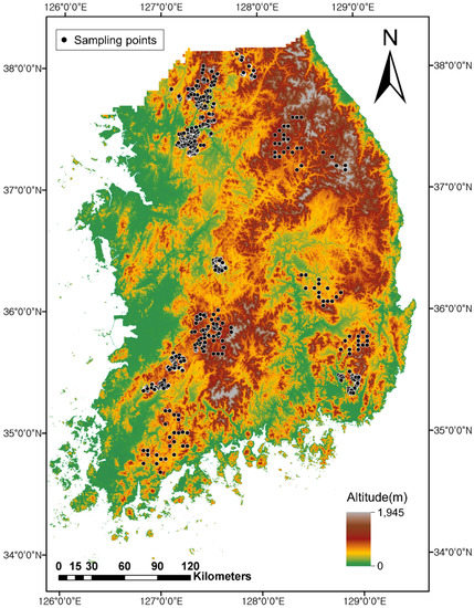
Figure 1. Distribution of collected forest soils in South Korea (1456 soil samples).

2.2. Soil Physical Properties and Topographic Features

Forest soil samples were collected through a 100 cc soil core sampler, and a total of 1456 soil samples were collected throughout the forest nationwide. Six properties were analyzed through laboratory experiments to investigate the physical properties of the soil. The analyzed soil properties were the saturated hydraulic conductivity; bulk density; sand, silt, and clay fraction; and organic matter (Table 1). The distribution of the 1456 soils across the USDA (United States Department of Agriculture) textural classes and the range of saturated hydraulic conductivity ($K_s$) by textural class are shown in Figure 2.

Table 1. Descriptive statistics for forest soil properties.

Soil Properties	Abb.	Unit	Min	Mean	Max	Std.	Skew.	Kurt.
Logarithmized Saturated Hydraulic Conductivity	Ln($K_s$)	cm day−1	0.37	6.57	8.98	1.21	−1.12	4.60
Bulk density	${\rho }_b$	g cm−3	0.45	1.03	1.59	0.19	0.12	2.78
Sand fraction	Sand	%	6.24	43.64	90.96	15.39	0.22	2.62
Silt fraction	Silt	%	1.46	33.01	81.36	12.66	0.07	2.39
Clay fraction	Clay	%	3.21	23.35	86.72	9.96	1.47	7.56
Organic matter	OM	%	2.08	9.16	29.71	3.53	1.09	4.94

Abbreviations: Abb, abbreviation; Std, standard deviation; Skew, skewness; Kurt, kurtosis.

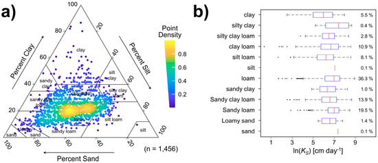
Figure 2. (a) Distribution of forest soils used in this study (n = 1456) across USDA textural classes and (b) ranges of the saturated hydraulic conductivity ($K_s$) and percent database by soil texture class.

The elevation, slope, topographic wetness index (TWI; Equation (2)), upper catchment area (CA), plan curvature, and profile curvature were collected as the topographic features. The elevation and slope indicate the altitude and local slope at the site where the soil was collected, respectively. The topographic wetness index, also known as the compound topographic index (CTI), indicates the steady state wetness index by topographic features. The TWI is calculated by the local upper catchment area and local slope and is derived as follows:

$$\mathrm{TWI}=\frac{a}{tanb}$$

(1)

where a is the local upper catchment area draining through a certain point per unit contour length and $tanb$ is the local slope [20]. The plan curvature can represent the shape of the horizontal plane, and the profile curvature can represent the shape of the vertical plane. The TWI, plan curvature, and profile curvature were calculated with the GIS spatial analyst tool.

In addition, the characteristics of the forest stand and site from which the soil samples were collected were investigated. The forest stand was divided into three categories: coniferous forest, broadleaf forest, and mixed forest. Bedrock and landform were investigated as site characteristics. Bedrock was largely divided into five types, including igneous, sedimentary, and metamorphic rock, and landform was classified into five types, as defined in Table 2.

Table 2. Landform classification.

Classification	Definition
Flat	A flat area with a slope of less than 5 degrees
Gentle slope	A hill with a slope of less than 300 m
Lower concave segment	The lower part of the mountain with a concave shape
Cliff face	The middle part of the mountain with a slope
Upper convex segment	The upper part of the mountaintop

2.3. Multiple Linear Regression for PTFs

2.3.1. Pedo-Transfer Functions (PTFs) in Previous Research

We selected PTFs that have frequently been cited in the literature for comparing the $K_s$ of forest soils in South Korea to the $K_s$ from other international databases by estimating the saturated hydraulic conductivity using our database. Six PTF models were selected, and brief explanations and references are shown in Table 3. Subsequently, the forest soil characteristics of South Korea were compared with other soil conditions by comparing the measured and predicted saturated hydraulic conductivity, which were estimated by six PTFs with the measured soil physical characteristics as input data.

Table 3. Six pedo-transfer functions (PTFs; Equations (S1)–(S6)) of previous research used for estimating the saturated hydraulic conductivity and their required soil properties.

Reference	${\mathit{K}}_{\mathit{s}}\mathbf{Unit}$	Required Soil Properties for Estimation	Land Use Types
Puckett et al. [12]	mm h−1	Clay	The lower coastal plain
Campbell and Shiozawa [21]	mm h−1	Sand, Clay	na
Jarbro [11]	cm day−1	Silt, Clay, ${\rho }_b$	na
Dane and Puckett [17]	mm h−1	Clay	The lower coastal plain
Wosten et al. [15]	cm day−1	Silt, Clay, Organic matter, ${\rho }_b$	na
Julia et al. [14]	mm h−1	Sand, Clay, Organic matter	na

Note: ${\rho }_b$ is the bulk density and na is not available. Soil databases from many previous studies were based on various land use types, so there was no clear information about land use types.

Six PTFs did not focus on the forest soil, and many previous studies were based on various land use types. There was also no clear information about the land use types because previous research was conducted primarily focusing on local regions in which soil surveys were carried out. The PTFs in previous research have been empirical equations. Therefore, the ranges of the soil properties from which each PTF was derived are represented in Table 4.

Table 4. Brief descriptive statistics for soil properties in previous research.

Soil Properties		Puckett et al.	Campbell and Shiozawa	Jarbro	Dane and Puckett	Woesten et al.	Julia et al.	This Study
Sand (%)	min	34.6	9.0	17.0	34.6	0.8	14.0	6.2
	max	88.5	89.0	96.0	88.5	58.0	94.2	91.0
Silt (%)	min	7.4	na	0.2	7.4	0	na	1.5
	max	35.8		52.0	35.8	23.3		81.4
Clay (%)	min	1.4	5.0	1.0	1.4	0	2.3	3.2
	max	42.1	47.0	44.0	42.1	18.7	54.1	86.7
Bulk density (g cm−3)	min	1.52	na	1.26	1.52	0.95	na	0.45
	max	1.86		1.97	1.86	1.58		1.59
$ln\left(K_s\right)$ (cm day−1)	min	na	na	−2.90	na	−0.76	na	0.37
	max			8.34		3.91		8.98

Note: na is not available.

2.3.2. Preprocessing of Explanatory Variables

In this study, PTFs were developed with multiple linear regression analysis to estimate the logarithmized saturated hydraulic conductivity ($ln\left(K_s\right)$). Since the saturated hydraulic conductivity can have a non-linear relationship with soil characteristics and topographic features, logarithmized ($\ln \left(x\right)$), exponential ($e^x$), squared ($x^2$), and untreated (x) treatments were carried out, and linear correlations with $\ln \left(K_s\right)$ were compared. Subsequently, the most linearly correlated variable type was adopted as the explanatory variable for multiple linear regression. The Pearson correlation coefficient was used to confirm the linear correlation.

2.3.3. Detecting Multicollinearity Using the Variance Inflation Factor (VIF)

In multiple linear regression, when there is a correlation between variables, coefficients in the multiple regression equation can be unreasonable and unreliable values, which is called a multicollinearity problem. Because this happens when a linear correlation occurs between the explanatory variables, it is necessary to remove the highly correlated variable in order to produce a reasonable result [22]. The variance inflation factor (VIF) is one of the best methods for identifying the correlation between variables. Since the VIF is a numerical value after multiple linear regression analysis is performed between explanatory variables, the higher the linear correlation between the explanatory variables, the higher the value of the VIF. If the VIF is higher than 5, it is determined that there is multicollinearity and the variable is removed [23]. The variance inflation factor (VIF) for one explanatory variable ($x_1$) is derived as follows:

$${\mathrm{VIF}}_{x_1}=\frac{1}{1-R_{x_1}^2}$$

(2)

where $R^2$ is the coefficient of determination of the multiple regression equation, which is estimated with one variable $x_1$ as a response variable and other variables as explanatory variables.

2.4. Model Assessment

Seventy percent of the total data set was used for developing the PTFs, and the remaining 30%, the hold-out test data set, was used to verify the model. To assess the performance of the PTF model developed in each process, the root mean squared log-transformed error (RMSLE), mean log-transformed error (MLE), and coefficient of determination ($R^2$) were used, and these are defined as follows:

$$\mathrm{RMSLE}=\sqrt{\frac{1}{N}{\displaystyle \sum }_{i=1}^N{\left[\ln {\left(\widehat{K_s}\right)}_i-\ln {\left(K_s\right)}_i\right]}^2}$$

(3)

$$\mathrm{MLE}=\frac{1}{N}{\displaystyle \sum }_{i=1}^N\left|\ln {\left(\widehat{K_s}\right)}_i-\ln {\left(K_s\right)}_i\right|$$

(4)

$$R^2=1-\frac{{{\displaystyle \sum }}_{i=1}^N{\left[\ln {\left(\widehat{K_s}\right)}_i-\ln {\left(K_s\right)}_i\right]}^2}{{{\displaystyle \sum }}_{i=1}^N{\left[\ln {\left(\overline{K_s}\right)}_i-\ln {\left(K_s\right)}_i\right]}^2},$$

(5)

where n is the number of observation samples, $K_s$ is the measured saturated hydraulic conductivity, $\widehat{K_s}$ is the predicted value from the PTFs, and $\overline{K_s}$ is the mean of the measured values. The RMSLE and MLE represent the differences between the measured and predicted values as absolute values, and the lower the performance of the model, the higher the values. The RMSLE is directly affected by the scale factor and reacts more sensitively to outliers than the MLE. $R^2$ is the dimensionless value that represents the correspondence between the measured data and the predicted data. This has a value between 0 and 1, and variables are more correlated as the $R^2$ nears 1.

2.5. Sensitivity Analysis

Sensitivity analysis can determine the effect of each explanatory variable on the response variable by confirming the amount of change in the response variable as the explanatory variable changes [24]. The coefficient of multiple linear regression (MLR) can represent the sensitivity of the variable because the explanatory and response variables have a linear relationship. Therefore, it is not necessary to conduct sensitivity analysis if MLR is adopted as a model. However, in this study, several MLRs were presented, not just one MLR, to estimate the saturated hydraulic conductivity. Additionally, each explanatory variable had nonlinearity throughout the preprocessing.

Each explanatory variable was varied by total 10 multipliers: 0.1, 0.25, 0.5, 0.8, 0.9, 1.1, 1.2, 2, 4, and 10. Each variable was multiplied while the others were kept constant. Moreover, the multiplied variable was used as the input variable in PTFs, and the output, which was the modified saturated hydraulic conductivity, was normalized (modified $ln\left(K_s\right)$/non-treated $ln\left(K_s\right)$) to determine the amount of change. A sensitivity run was only implemented once for the PTF model, because there was no variance between the output of each sensitivity run.

Statistical analyses, such as the Pearson correlation analysis, analysis of variation (ANOVA), multiple linear regression, and p-value determination, were conducted using the SPSS software. We confirmed that the result was statistically significant and rejected the null hypothesis when the p-value was less than 0.05.

3. Results

3.1. Saturated Hydraulic Conductivity in Forest Soil

Six PTFs were analyzed to confirm the difference between the $K_s$ of the forest soil collected in this study and the $K_s$ predicted by the PTFs in previous research. The $K_s$ was calculated using 1456 soil physical characteristics as input factors for the PTFs in previous research. Six PTFs did not focus on the forest soil, and many previous studies were based on various land use types. There was also no clear information about land use types. Figure 3 also shows the predicted $K_s$ from the PTFs in previous research and measured $K_s$ in this study. Figure 3 shows the range of the logarithmized $K_s$ on the left side and its probability density function on the right side.

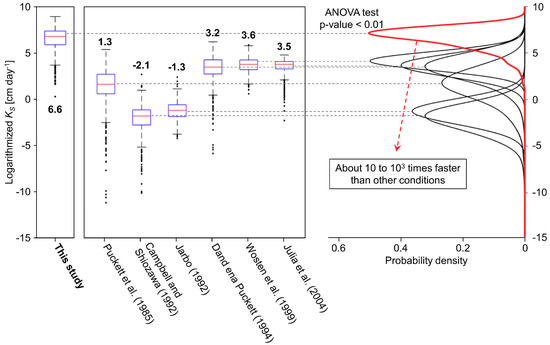
Figure 3. Mean values and ranges of the observed logarithmized $K_s$ (saturated hydraulic conductivity) of forest soil in South Korea (this study), predicted logarithmized $K_s$ based on PTFs presented in the literature, and kernel probability density functions of these logarithmized $K_s$. Six PTFs did not focus on the forest soil, and there are different ranges of the soil properties that previous research used.

The averaged logarithmized $K_s$ of the forest soil was 6.6, and the average logarithmized $K_s$ from the six PTFs using the same input data set varied from −2.1 to 3.6. The $K_S$ of the forest soil that was observed in this study was about 10 to 10³ times larger than the $K_s$ predicted with the PTFs of previous research. Additionally, most of the predictions exhibited negative $ln\left(K_s\right)$, which means that the $K_s$ was between 0 and $e$ cm day⁻¹ and thus very low. In this study, however, no negative values were observed. The ANOVA test also showed that the $K_S$ of the forest soil was higher than the $K_s$ predicted by previous research for forest soils, which was statistically significant. Considering the range of the soil properties in Table 4, the range of the soil size distribution is different. In particular, the bulk density of the forest soil is lower than the bulk density of the soils used in previous research. These discrepancies indicate differences of $K_s$, and the PTFs were difficult to use to rationally explain the $K_S$ of the forest soil in South Korea.

3.2. Explanatory Variable Selection

The most appropriate treatment of the explanatory variables was selected to estimate $K_s$ through soil characteristics and topographic features. For selecting the appropriate treatment, logarithmized ($ln\left(x\right)$), exponential ($e^x$), squared (x²), and untreated treatments (x) were carried out for each variable, and the linear correlation with $ln(K_s)$ of each treatment was compared. Table 5 shows the best results of the correlation analysis of the explanatory variables. Among the soil properties, sand and organic matter had a higher linear correlation when logarithmized, and silt and clay had a higher correlation when squared (Table 5). In terms of the topographic features, the TWI was highly correlated with logarithmized treatment and CA was highly correlated when squared after being logarithmized. The p-value of all the variables was statistically significantly correlated with the logarithmized $K_s$ (p < 0.05), and the bulk density and organic matter showed a strong linear relationship.

Table 5. Relationship between $ln\left(K_s\right)$ and the best treatment of explanatory variables.

Selected Explanatory Variables		PCC	p-Value	VIF before the Removal	Multi-Collinearity	VIF after the Removal
Soil properties	${\rho }_b$ (-)	−0.46	<0.01	2.25	X	2.25
	ln(sand) (%)	0.14	<0.01	16.67	O	1.67
	Silt2 (%)	−0.08	<0.01	12.78	O; removed	-
	Clay2 (%)	−0.14	<0.01	7.87	O	1.48
	ln(OM) (%)	0.26	<0.01	1.89	X	1.87
Topographic feature	Elevation (m)	−0.05	0.039	1.21	X	1.17
	Slope (%)	−0.23	<0.01	1.11	X	1.11
	ln(TWI) (-)	0.09	<0.01	1.46	X	1.46
	(ln(CA))2 (m2)	0.07	<0.01	1.07	X	1.07
	Plan curvature	−0.08	<0.01	3.77	X	3.77
	Profile curvature	−0.08	<0.01	3.84	X	3.83

Note: PCC is the Pearson correlation coefficient and VIF is the variance inflation factor. The silt variable was removed because of the multicollinearity problem. After the removal, there was no multicollinearity in the variables (VIF < 5).

The VIF is calculated with both soil and topographic features, and values greater than 5 were found in the sand, silt, and clay fractions. This is because the sand, silt, and clay fractions are factors that are organically related to each other, so one of these factors must be removed to solve this multicollinearity problem. Sand was logarithmized, but silt and clay were squared, so sand might have a weaker linear correlation with silt and clay. Therefore, silt was removed, since silt had higher VIF values than clay. After removing silt, the VIF values of all the variables were less than 5, which indicates that there is no multicollinearity problem.

3.3. Categories with Statistical Analysis

Forest soil is affected by various forest stand and site characteristics, in addition to the soil and topographic features given in Table 6. Therefore, we analyzed the differences in $K_s$ by forest type, bedrock, landform, and soil layer (Table 6). The forest types were divided into three types: coniferous, broadleaved, and mixed forest. Moreover, bedrock was classified into igneous, sedimentary, and metamorphic rock. Landform was classified into five categories (Table 2), and the soil layers were classified as topsoil and subsoil.

Table 6. The $K_s$ differences by forest type, bedrock, landform, and soil layer obtained by ANOVA.

Classification		N	${\mathit{K}}_{\mathit{s}}$	$\mathit{l}\mathit{n}\left({\mathit{K}}_{\mathit{s}}\right)$	Post Hoc Analysis	F-Value	p-Value
Forest type	Coniferous	714	632.70	6.45	a	14.14	<0.01
	Broadleaf	550	796.32	6.68	b
	Mixed	192	812.41	6.70	b
Bedrock	Igneous	331	658.52	6.49	a	13.46	<0.01
	Sedimentary	329	454.86	6.12	a
	Metamorphic	796	888.91	6.79	b
Landform	Flat	175	454.86	6.12	a	20.38	<0.01
	Gentle slope	209	550.04	6.31	a
	LCS	633	992.27	6.90	b
	Cliff face	237	658.52	6.49	a
	UCS	202	487.85	6.19	a
Soil layer	Topsoil	728	880.07	6.78	a	20.99	<0.01
	Subsoil	728	578.25	6.36	b

Note: LCS is the lower concave segment, UCS is the upper convex segment, and n is the number of samples. Forest type, bedrock, landform, and soil layer exhibit significant differences in $K_s$ (p < 0.01). Post hoc analysis was conducted with Tukey’s method, and bold values have higher $K_s$ than others. ANOVA was conducted with the SPSS statistic software package.

According to ANOVA analysis and Tukey’s post hoc analysis, the soil located in broadleaf and mixed forest had a higher saturated hydraulic conductivity than the soil located in coniferous forest (p < 0.01). Furthermore, the soil with metamorphic rock as a bedrock had a higher saturated hydraulic conductivity than the soil with igneous and sedimentary rock (p < 0.01). By landform classification, the soil located in the lower concave segment was statistically significantly higher than that in others (p < 0.01), with no statistical differences in the other four landforms except the lower concave segment. Moreover, the topsoil had a higher $K_s$ than subsoil (p < 0.01).

The overall data set was divided into several categories because there were statistically significant differences in $K_s$ by forest type, bedrock, landform, and soil layer, as shown in Table 6. As a result of the post hoc analysis of the forest type, bedrock, landform, and soil layer, all of the four forest stands and site characteristics could be classified into two categories: relatively fast $K_s$ and relatively slow $K_s$. The total data set, therefore, was classified into 16 categories, depending on the characteristics of the forest type, bedrock, landform, and soil layer (Table 7).

Table 7. Sixteen categories based on forest stand, geological, and topographical features.

Categories	Forest Type	Bedrock	Landform	Soil Layer	Number of Soil Samples
1	Coniferous	I & S	Other LF	Subsoil	130
2	Coniferous	I & S	Other LF	Topsoil	132
3	Coniferous	I & S	L.C.S.	Subsoil	51
4	Coniferous	I & S	L.C.S.	Topsoil	51
5	Coniferous	Metamorphic	Other LF	Subsoil	84
6	Coniferous	Metamorphic	Other LF	Topsoil	84
7	Coniferous	Metamorphic	L.C.S.	Subsoil	91
8	Coniferous	Metamorphic	L.C.S.	Topsoil	91
9	B & M	I & S	Other LF	Subsoil	109
10	B & M	I & S	Other LF	Topsoil	110
11	B & M	I & S	L.C.S.	Subsoil	39
12	B & M	I & S	L.C.S.	Topsoil	38
13	B & M	Metamorphic	Other LF	Subsoil	87
14	B & M	Metamorphic	Other LF	Topsoil	87
15	B & M	Metamorphic	L.C.S.	Subsoil	137
16	B & M	Metamorphic	L.C.S.	Topsoil	135

Abbreviations: B & M, broadleaf or mixed forest; I & S, igneous or sedimentary bedrock; Other LF, four landforms except the lower concave segment; L.C.S., lower concave segment (Table 2).

3.4. Development of the Pedo-Transfer Function

The soil data were classified into 16 categories, and multiple linear regression analysis was conducted for each category. Since most PTF studies have only been conducted with soil characteristics to date, multiple linear regression analysis was conducted twice: with soil characteristics only and with soil characteristics and topographic features. Table 8 shows the results of multiple linear regression analysis with only soil characteristics as the input data. Additionally, Table 9 shows the results of multiple linear regression analysis with topographic features in addition to soil characteristics. Table 8 and Table 9 show the regression coefficients of each variable according to multiple linear regression, and full equations are available in the Supplementary Materials (Table S1 and S2).

Table 8. Regression coefficients of categorical PTFs for the logarithmized saturated hydraulic conductivity with only soil properties.

	1	2	3	4	5	6	7	8	9	10	11	12	13	14	15	16
${\rho }_b$	−4.899	−3.988	−4.274	−2.890	−3.163	−3.452	−4.875	−1.325	−3.852	−3.939	−6.909	−4.797	−4.589	−2.265	−1.693	−0.666
ln(Sand)	0.803	0.748	1.553	0.690	0.634	0.889	1.867	1.269	0.858	0.543	−0.003	−0.248	0.731	0.502	0.768	−0.300
Clay2 *	1.752	1.094	6.362	0.004	1.129	2.227	−1.251	−1.255	2.435	1.116	−5.136	−6.104	1.064	3.735	2.554	−2.392
ln(OM)	−0.158	0.314	1.201	−0.219	−0.516	−0.016	−0.470	0.073	−1.209	−0.852	−1.934	−0.766	−1.764	−0.659	−0.124	−0.019
Intercept	8.730	7.042	2.570	7.207	8.503	6.615	5.758	3.374	9.527	10.433	18.003	14.270	11.948	8.270	5.942	9.317

Note: Clay2 * is clay2 $\times$ 10⁻⁴. The regression coefficients of clay2 were too small, so the constant was multiplied to make them readable. In total, 16 categories were classified according to Table 7, and these values are the regression coefficients from multiple linear regression.

Table 9. Regression coefficients of categorical PTFs for the logarithmized saturated hydraulic conductivity with topographic features in addition to soil properties.

Categories	1	2	3	4	5	6	7	8	9	10	11	12	13	14	15	16
${\rho }_b$	−3.499	−2.753	−3.147	−3.531	−2.385	−3.157	−3.402	−0.991	−4.559	−3.945	−4.622	−3.496	−3.675	−2.469	−1.793	−0.774
ln(Sand)	1.018	1.168	0.955	0.793	0.524	0.637	1.159	1.029	0.930	0.724	−0.865	0.006	1.323	0.686	1.233	−0.118
Clay2 *	1.266	2.294	−3.235	−2.111	−2.267	−0.532	−4.992	−1.668	2.473	3.831	−9.888	−3.558	3.744	7.769	4.963	−1.178
ln(OM)	0.978	1.035	0.215	0.669	0.002	−0.386	0.186	0.204	−1.055	−1.368	−1.402	−0.412	−0.675	−0.927	−0.205	0.012
Elevation *	−0.505	−1.193	0.348	−0.929	0.398	0.546	−1.006	−0.127	−0.466	−0.348	0.882	3.129	−1.409	−0.675	−1.291	−0.031
Slope	−0.031	−0.041	−0.051	−0.060	−0.030	−0.027	−0.014	−0.019	−0.034	−0.007	−0.104	−0.060	−0.002	0.005	−0.017	0.000
ln(TWI)	−0.078	−0.049	−0.263	−0.284	0.128	0.062	0.007	−0.079	0.133	0.047	0.205	−0.116	0.248	0.253	−0.006	0.039
CA2 *	−0.208	0.530	1.136	1.097	0.354	1.449	0.754	1.232	0.021	0.615	−1.471	0.503	1.227	2.011	−0.418	0.207
Plan curvature	0.903	0.281	−0.001	−1.342	0.921	−0.838	0.312	−0.124	−1.077	−2.362	−0.021	0.690	0.360	−0.388	−0.089	−0.560
Profile curvature	−0.448	−0.312	−0.392	0.574	−0.433	0.660	0.049	0.249	0.725	1.432	−0.642	−1.495	0.145	0.672	−0.170	0.182
Intercept	5.260	3.769	7.480	7.714	7.386	8.366	6.123	4.108	10.514	10.847	19.924	11.621	5.714	7.264	5.145	8.404

Note: Clay² * is clay² $\times$ 10⁻⁴; elevation* is elevation $\times$ 10⁻³; CA² * is CA² $\times$ 10⁻². The regression coefficients of clay², elevation, and CA² were too small, so the constant was multiplied to make them readable. In total, 16 categories were classified according to Table 7, and these values are coefficients from multiple linear regression.

Figure 4 shows the measured and predicted $K_s$ with the developed PTFs with 16 categories. The model was developed using 70% of the total data set and validated with the remaining hold-out test data set. In the calibration phase, the coefficient of determination with only soil properties was 0.37 but increased to 0.43 when topographic features were added as input data. Moreover, the coefficient of determination values, 0.37 and 0.43, are significantly different from 0. The model performance also increased in the validation phase. The RMSLE and MLE, which show the deviation of the measured and predicted values, also decreased from 0.931 and 0.724 to 0.920 and 0.709, respectively. The model performance was improved when topographic features were taken into account in both calibration and validation.

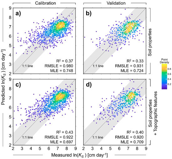
Figure 4. Relationship between the measured and predicted logarithmic $K_s$ value. Multiple linear regressions were conducted with the calibration data set, which represented 70% of the total data set, and validated by the validation data set, which consisted of the rest of the data. (a,b) show analysis with only soil properties, and (c,d) show analysis with topographic features in addition to soil properties. The grayed-out parts are the ranges of the 95% prediction interval limits of the 1:1 lines.

3.5. Model Sensitivity

Ten variables were analyzed for sensitivity analysis, and four highly sensitive variables were selected (Figure 5). All multipliers were not applied to variables having the upper limit. For example, for the sand fraction, since the maximum value of the sand fraction is 100%, the sensitivity analysis was performed up to multiplier 4. Sensitivity analysis showed that the bulk density and sand fraction, which are soil properties, and the slope and catchment area, which are topographic features, had the great effect on $K_s$. $K_s$ was increased when the sand fraction and catchment area increased, and $K_s$ was decreased when the bulk density and slope increased. However, clay, organic matter, elevation, TWI, plan curvature, and profile curvature did not significantly affect the $K_s$.

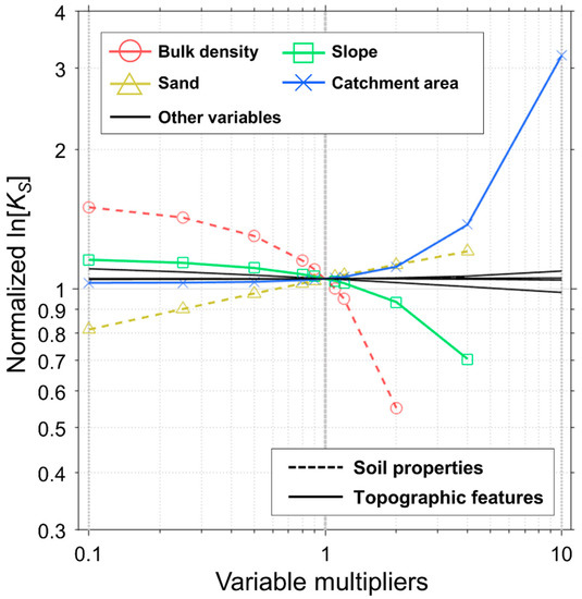
Figure 5. Sensitivity results for logarithmized $K_s$. Only the four most sensitive variables are colored, and the variables of soil properties are shown with dashed lines. Large vertical differences from the line y = 1 indicate a relatively high sensitivity for estimating the saturated hydraulic conductivity.

4. Discussion

4.1. Different Characteristics of K_S in Forest Soil

Figure 3 shows the use of the PTFs from previous research to estimate the $K_s$ of the forest soil. The measured $K_s$ was more than 10 times larger than the $K_s$ predicted by previous research. Using the PTFs of previous research can therefore lead to the underestimation of the $K_s$ of forest soil. Because they did not focus on the forest soil and the ranges of the soil properties used for developing the PTFs were different. Unlike the soil of cultivated land, grassland, or bare land, forest soil is not compacted and large and small pores are widely distributed. Therefore, forest soil has a relatively low bulk density. As presented in Table 4, the ranges of the soil size distribution in previous research and this study are similar. On the other hand, the bulk density of the forest soil in South Korea was smaller and beyond the range of previous research. This could be one of the reasons for the higher $K_s$ of forest soil in South Korea.

In forests, various types of plants are growing and have a great influence on the soil hydrology [25,26]. Piaszczyk et al. [27] showed that dead trees in forests can have a great impact on the soil’s physical properties. Furthermore, some studies have shown that organic matter produced from the roots of trees or understory plants in forests has a significant impact on the physical structure of forest soil [22,23,28]. Due to these characteristics, forest soil has a high permeability.

4.2. K_S Differences by Forest Stand, Geological, and Topographical Features

Forest soil can be affected by a number of topographical factors and the type of forest stand. As shown in Table 6, it was found that differences in the $K_s$ by forest stand, bedrock, and landform were statistically significant. First, there was a difference in the $K_s$ for different forest stands, where the $K_s$ of broadleaf and mixed forests was higher than that of coniferous forest. The type of forest can have a great influence on the soil hydrology [25]. This can be explained by the root distribution difference between coniferous and broadleaf trees. Burch [24] demonstrated that coniferous trees have straight roots in a vertical direction, while broad-leafed trees spread wide in the lateral direction and produce a large number of rootlets. In other words, in the case of broadleaf and mixed forests, it is assumed that the pores of the soil are more advanced than those of coniferous forests due to the root system of trees, and thus, broadleaf and mixed forests have higher $K_s$. Secondly, almost all of the broadleaf trees in South Korea are deciduous trees, which can produce a thicker litter layer than coniferous trees. Litter layers can produce higher organic carbon contents, which are related to lower bulk densities [27,29], so the $K_s$ increases.

Soil is made by weathering from the bedrock. Therefore, soil properties are highly affected by the bedrock. Plaster and Sherwood [30] showed that soil from metamorphic rock can include a high rate of the sand fraction. On the other hand, soil with fine particles is produced from sedimentary rock. Table 6 shows that the soil from sedimentary rock had the lowest $K_S$, and the soil from metamorphic rock had the highest $K_s$. The 1456 samples of forest soil also showed that the sand fracture contents were 40.6%, 35.6%, and 48.2% in igneous, sedimentary, and metamorphic rock, respectively, from which it was confirmed that soil from metamorphic rock has the highest permeability. This is consistent with the analysis of previous research [30].

The $K_s$ of forest soil also differed, depending on the landform. The lower concave segment is the part where the soil does not erode but is deposited, unlike other landforms. As the soil is deposited, the soil is not compacted, so there is a lot of space for water to move in the soil, which is the reason for the high $K_s$. The 1456 samples showed a lower bulk density in the lower concave segment than other landforms. Martin [31] also identified that the soil property changes were those associated with the downward movement of water and soil, and there was a deeper topsoil depth and higher organic matter content in the lower concave segment, which is the lower part of the mountain. These differences can lead to high $K_s$. Topsoil and subsoil also showed a difference in $K_s$. Subsoil is located below topsoil, so the soil compaction derived from the gravity leads to lower $K_s$. The subsoil soil layer also has lower organic matter contents than topsoil, which can lead to higher bulk densities and lower and lower $K_s$ [27,29]. In this study, topsoil contained 2.5% more organic matter than subsoil.

Forest soil is affected by various topographical factors, such as the forest type, bedrocks, and the landform directly related to the erosion and sedimentation. Therefore, in order to understand the characteristics of the $K_s$, all of these factors must be considered and analyzed.

4.3. Relationship between K_S and Soil and Topographic Features

The relationship between $K_s$ and soil and topographic features can be found in Table 8 and Table 9. If the coefficient is positive, the variable is positively correlated with the $K_s$. Therefore, $K_s$ increases as the sand fraction and upper catchment area increase, and $K_s$ decreases as the bulk density, elevation, and slope increase. The sand fraction and bulk density are directly related to the porosity. Therefore, a higher sand fraction and lower bulk density result in a high porosity, which can lead to a higher $K_s$. The lower the elevation, the higher the $K_s$, and this can be explained by the erosion and deposition process in the mountain slope. In other words, a low elevation area is also the part where the forest soil is deposited, so the soil layer is getting deeper and a higher porosity can be formed [32]. However, it can be highly related to the relationship between the elevation and other topographic features. In the lower concave segment, the $K_s$ is higher than that of other landform types (Table 6). This could be the major reason for the negative relationship between the $K_s$ and the elevation, and further research is needed to clarify the effects of the elevation on the $K_s$. The slope and catchment area can also be explained by similar reasons. The erosion progresses as the slope increases; on the other hand, deposition progresses as the slope decreases. Additionally, as the upper catchment area increases, more water and soil are transported down the hill. In other words, the lower the elevation and the lower the slope, which is related to the bigger upper catchment area, the deeper the soil layer and the lower the bulk density, which leads to higher $K_s$.

The organic matter, TWI, plan curvature, and profile curvature, however, did not significantly affect the $K_s$. Nemes [33] explained that the organic matter in soil may increase the total porosity of the soil, thereby increasing the hydraulic conductivity, but in contrast, it can reduce the $K_s$ by retaining the water. In other words, one measure of organic matter contents alone cannot fully explain the $K_s$ since the effect of organic matter on the $K_s$ of forest soil is complex. The TWI, plan curvature, and profile curvature were also used as important factors for estimating the moisture content of soil, which is one of the most important soil properties [34]. However, it was found that these factors did not have a significant role in explaining the $K_s$.

Figure 4 shows that the model’s performance increased when the topographic features were added, which can be confirmed through the sensitivity analysis (Figure 5). Four highly sensitive variables are the bulk density, sand fraction, slope, and catchment area, which can explain the $K_s$ well. The bulk density and sand fraction are soil properties, but the slope and catchment area, which are topographic features, also highly affected the $K_s$. In other words, it can be seen that $K_s$ is not only directly affected by soil properties but also greatly affected by topographic features. Therefore, topographic features should be considered when forest soil characteristic analyses are carried out.

4.4. Limitations and Suggestions for Future Research

In this study, non-linearity was considered by conducting the preprocessing of 10 soil and topographic characteristic variables to estimate $K_s$. Furthermore, 16 categories were divided through statistical analysis and the linear relationship with $K_s$ was analyzed for each category. We confirmed that the soil properties and topographic features highly affect the $K_s$ of forest soil in this study. In South Korea, a soil investigation is being conducted on a national scale. With these database and topographic data, the $K_s$ can be estimated on a national scale by using the PTFs. Because a lot of hydraulic simulation models use the $K_s$ as an important input variable, these PTFs can be useful for running these models and for understanding the water cycle.

This model, however, still does not have a high performance. This is because the $K_s$ of forest soil is affected by more site and environmental factors than the above variables used in this study. Moreover, it is difficult to explain all of these nonlinear relationships with simple multiple linear regression. Therefore, it may be possible to construct a model with a higher performance when the other factors highly related to the $K_s$ are found and analyzed. Recently, machine learning has been used to develop a model that predicts the $K_s$, in which case the performance of the model is increased [1,34]. However, the machine learning model is difficult to access for other researchers, so it is not easily available for other researchers. For these reasons, the machine learning model was not covered in this paper. Further research can use artificial intelligence and deep learning technology to check the nonlinear relationship between the $K_s$ and various topographical factors in forest soil, and then use several nonlinear models to develop PTFs with a high performance. In addition, it is expected that a more accurate prediction of $K_s$ on a national scale can be conducted when artificial intelligence and the deep learning model is developed using these forest soil data.

5. Conclusions

In South Korea, forest covers about two-thirds of the land area of the whole country. Due to these geographical characteristics, understanding the soil properties in forests is important for sustainable water management. The $K_s$ is one of the most important input variables for running a hydraulic simulation model. Therefore, developing PTFs for predicting the $K_s$ is necessary. In this study, data from 1456 sampling points were collected throughout South Korea, which are located in the temperate climate zone, and PTFs to predict the $K_s$ from soil and topographic features were developed. The $K_s$ of the broadleaf and mixed forests was higher than that of the coniferous forests, which is because of the root characteristic differences and the litter layer by forest type. The $K_s$ of the soil based on igneous and sedimentary rocks was higher than that of the soil based on metamorphic rocks. This is because of the formation of sandy soil during the weathering of metamorphic rocks. In addition, soil located in the lower concave segment had a lower bulk density and higher $K_s$ because the soil located in the lower concave segment is deposited rather than eroded, unlike other landforms. Furthermore, the $K_s$ of subsoil was lower than that of topsoil due to soil compaction by gravity and organic matter contents. Many previous researchers have only considered soil properties to predict the $K_s$. However, since forests display spatial variability, topographic features should be considered, in addition to soil properties. The PTF model performance increased when topographic features were added. As a result, the $K_s$ of the forest soil was increased when the bulk density, clay, elevation, and slope were decreased and the sand fraction and upper catchment area were increased. The organic matter, TWI, plan curvature, and profile curvature did not highly affect the $K_s$ of the forest soil. According to the sensitivity analysis, the bulk density, sand fraction, slope, and catchment area highly affected the $K_s$. Therefore, the topographic features were as important in predicting the $K_s$ as the soil properties of the forest soil.

References

- Araya, S.N.; Ghezzehei, T.A. Using machine learning for prediction of saturated hydraulic conductivity and its sensitivity to soil structural perturbations. Water Resour. Res. 2019, 55, 5715–5737. [Google Scholar] [CrossRef]
- Du, E.; Link, T.E.; Gravelle, J.A.; Hubbart, J.A. Validation and sensitivity test of the distributed hydrology soil-vegetation model (DHSVM) in a forested mountain watershed. Hydrol. Process. 2014, 28, 6196–6210. [Google Scholar] [CrossRef]
- Simunek, J.; Van Genuchten, M.T.; Sejna, M. HYDRUS: Model use, calibration, and validation. Trans. ASABE 2012, 55, 1263–1274. [Google Scholar]
- Beven, K. TOPMODEL: A critique. Hydrol. Process. 1997, 11, 1069–1085. [Google Scholar] [CrossRef]
- Kabat, P.V.; Van den Broek, B.J.; Feddes, R.A. SWACROP: A water management and crop production simulation model. ICID Bull. 1992, 2, 61–83. [Google Scholar]
- Wösten, J.H.M.; Pachepsky, Y.A.; Rawls, W.J. Pedotransfer functions: Bridging the gap between available basic soil data and missing soil hydraulic characteristics. J. Hydrol. 2001, 251, 123–150. [Google Scholar] [CrossRef]
- Keesstra, S.; Mol, G.; De Leeuw, J.; Okx, J.; De Cleen, M.; Visser, S. Soil-related sustainable development goals: Four concepts to make land degradation neutrality and restoration work. Land 2018, 7, 133. [Google Scholar] [CrossRef]
- Keesstra, S.D.; Bouma, J.; Wallinga, J.; Tittonell, P.; Smith, P.; Cerda, A.; Montanarella, L.; Quinton, J.N.; Pachepsky, Y.; Van Der Putten, W.H.; et al. The significance of soils and soil science towards realization of the United Nations Sustainable Development Goals. Soil 2016, 2, 111–128. [Google Scholar] [CrossRef]
- Bouma, J. Using soil survey data for quantitative land evaluation. Adv. Soil Sci. 1989, 9, 177–213. [Google Scholar]
- Wösten, J.H.M. Pedotransfer functions to evaluate soil quality. Dev. Soil Sci. 1997, 25, 221–245. [Google Scholar]
- Jabro, J.D. Estimation of saturated hydraulic conductivity of soils from particle size distribution and bulk density data. Trans. ASAE 1992, 35, 557–560. [Google Scholar] [CrossRef]
- Puckett, W.E.; Dane, J.; Hajek, B.F. Physical and mineralogical data to determine soil hydraulic properties. Soil Sci. Soc. Am. J. 1985, 49, 831–836. [Google Scholar] [CrossRef]
- Saxton, K.E.; Rawls, W.; Romberger, J.S.; Papendick, R.I. Estimating generalized soil-water characteristics from texture. Soil Sci. Soc. Am. J. 1986, 50, 1031–1036. [Google Scholar] [CrossRef]
- Julià, M.F.; Monreal, T.E.; del Corral Jiménez, A.S.; Meléndez, E.G. Constructing a saturated hydraulic conductivity map of Spain using pedotransfer functions and spatial prediction. Geoderma 2004, 123, 257–277. [Google Scholar] [CrossRef]
- Wösten, J.H.M.; Lilly, A.; Nemes, A.; Le Bas, C. Development and use of a database of hydraulic properties of European soils. Geoderma 1999, 90, 169–185. [Google Scholar] [CrossRef]
- Yang, H.; Choi, H.T.; Lim, H. Effects of forest thinning on the long-term runoff changes of coniferous forest plantation. Water 2019, 11, 2301. [Google Scholar] [CrossRef]
- Dane, J.H.; Puckett, W. Field soil hydraulic properties based on physical and mineralogical information. In International Workshop on Indirect Methods for Estimating the Hydraulic Properties of Unsaturated Soils; University of California: Riverside, CA, USA, 1994; pp. 389–403. [Google Scholar]
- Chirico, G.B.; Medina, H.; Romano, N. Functional evaluation of PTF prediction uncertainty: An application at hillslope scale. Geoderma 2010, 155, 193–202. [Google Scholar] [CrossRef]
- Young, M.H.; Caldwell, T.G.; Meadows, D.G.; Fenstermaker, L.F. Variability of soil physical and hydraulic properties at the Mojave Global Change Facility, Nevada: Implications for water budget and evapotranspiration. J. Arid Environ. 2009, 73, 733–744. [Google Scholar] [CrossRef]
- Sorensen, R.; Zinko, U.; Seibert, J. On the calculation of the topographic wetness index: Evaluation of different methods based on field observation. Hydrol. Earth. Syst. Sci. 2006, 10, 101–112. [Google Scholar] [CrossRef]
- Campbell, G.S.; Shiozawa, S. Prediction of hydraulic properties of soils using particle-size distribution and bulk density data. In International Workshop on Indirect Methods for Estimating the Hydraulic Properties of Unsaturated Soils; University of California: Riverside, CA, USA, 1992; pp. 317–328. [Google Scholar]
- Perie, C.; Ouimet, R. Organic carbon, organic matter and bulk density relationships in boreal forest soils. Can. J. Soil Sci. 2008, 88, 315–325. [Google Scholar] [CrossRef]
- Prévost, M. Predicting soil properties from organic matter content following mechanical site preparation of forest soils. Soil Sci. Soc. Am. J. 2004, 68, 943–949. [Google Scholar] [CrossRef]
- Burch, W.H.; Jones, R.H.; Mou, P.; Mitchell, R.J. Root system development of single and mixed plant functional type communities following harvest in a pine-hardwood forest. Can. J. Soil Sci. 1997, 27, 1753–1764. [Google Scholar] [CrossRef]
- Cerda, A.; Borja, M.E.L.; Ubeda, X.; Matinez-Murillo, J.F.; Keesstra, S. Pinus halepensis M. versus Quercus ilex subsp. Rotundifolia L. runoff and soil erosion at pedon scale under natural rainfall in Eastern Spain three decades after a forest fire. Forest Ecol. Manag. 2017, 400, 447–456. [Google Scholar] [CrossRef]
- Keesstra, S.D.; Van Dam, O.; Verstraeten, G.V.; Van Huissteden, J. Changing sediment dynamics due to natural reforestation in the Dragonja catchment, SW Slovenia. Catena 2009, 78, 60–71. [Google Scholar] [CrossRef]
- Piaszczyk, W.; Lasota, J.; Błońska, E. Effect of organic matter released from deadwood at different decomposition stages on physical properties of forest soil. Forests 2020, 11, 24. [Google Scholar] [CrossRef]
- Yue, C.; Huang, Y.; Wenjuan, S.U.N. Using organic matter and pH to estimate the bulk density of afforested/reforested soils in northwest and northeast China. Pedosphere 2017, 27, 890–900. [Google Scholar]
- Jonsson, B.G.; Ekström, M.; Esseen, P.A.; Grafström, A.; Ståhl, G.; Westerlund, B. Dead wood availability in managed Swedish forests-Policy outcomes and implications for biodiversity. Forest Ecol. Manag. 2016, 376, 174–182. [Google Scholar] [CrossRef]
- Plaster, R.W.; Sherwood, W.C. Bedrock weathering and residual soil formation in Central Virginia. Geol. Soc. Am. Bull. 1971, 82, 2813–2826. [Google Scholar] [CrossRef]
- Martin, W.K.E.; Timmer, V.R. Capturing spatial variability of soil and litter properties in a forest stand by landform segmentation procedures. Geoderma 2006, 132, 169–181. [Google Scholar] [CrossRef]
- Meinert, D.; Nigh, T.; Kabrick, J. Landforms, geology and soils of the MOFEP study sites. In Missouri Pzark Forest Ecosystem Project Symposium: An Experimental Approach to Landscape Research; General Technical Report NC-193; U.S. Forest Service, North Central Forest Experiment Station: St. Paul, MN, USA, 1997; pp. 56–68. [Google Scholar]
- Nemes, A.; Rawls, W.J.; Pachepsky, Y.A. Influence of organic matter on the estimation of saturated hydraulic conductivity. Soil Sci. Soc. Am. J. 2005, 69, 1330–1337. [Google Scholar] [CrossRef]
- Jin, X.; Wang, S.; Yu, N.; Zou, H.; An, J.; Zhang, Y.; Wnag, J.; Zhang, Y. Spatial predictions of the permanent wilting point in arid and semi-arid regions of Northeast China. J. Hydrol. 2018, 564, 367–375. [Google Scholar] [CrossRef]
© 2020 by the authors. Licensee MDPI, Basel, Switzerland. This article is an open access article distributed under the terms and conditions of the Creative Commons Attribution (CC BY) license (http://creativecommons.org/licenses/by/4.0/).