Application of Rehabilitation and Active Pressure Control Strategies for Leakage Reduction in a Case-Study Network

Abstract

The paper discusses the results of a simulation analysis to evaluate the potential of rehabilitation measures and active pressure control strategies for leakage reduction in a water distribution network (WDN) in southern Italy. The analysis was carried out by using a simulation model developed under the EPANET-MATLAB environment. The model was preliminarily calibrated based on pressure and flow measurements acquired during a field monitoring campaign in two districts of the WDN. Three different scenarios of leakage reduction including (i) pipe rehabilitation (scenario S1), (ii) implementation of pressure local control (S2), and (iii) introduction of remote real-time pressure control (RTC) (S3) were simulated and compared with the current scenario of network operation (S0). Results of the simulations revealed that a combination of the used strategies can improve network performance by a significant reduction of water leakage. Specifically, 16.7%, 35.0%, and 37.5% leakage reductions (as compared to S0) can be obtained under scenarios S1, S2, and S3, respectively.

1. Introduction

The level of service in water distribution networks (WDNs) is related to critical issues such as the frequency of breaks and the amount of background leakage in the network. Very often such issues are the cause of pressure drops in the network pipes, which are eventually detrimental to users’ water demand satisfaction [1]. Modeling of the network coupled with information gained through measurement of flows and pressures can significantly contribute to the identification of anomalies in the WDN and the proper estimation of leakage levels, as well as to the selection of actions for network rehabilitation and technological renewal [2,3].

For instance, strategies include methods for identifying pipes with high rehabilitation priority [4], as well as methods to reduce pressure (and, thus, leakage) in the WDN [5,6]. Pipe rehabilitation/replacement programs require acquiring knowledge about the characteristics of the pipes (typically, material, diameter, age, current status, and historical frequency of breaks) [7]. Most pressure control methods are based on dividing the WDN into district metered areas (DMAs) and on installing pressure control valves (PCVs) at their entrance for limiting pressure values in the downstream conduits [5]. Normally, PCVs allow local pressure control (they allow controlling the pressure value locally at the valve outlet) with the aim to control pressure levels in the whole downstream district. Therefore, local control relies on the use of hydraulic models of the network to predict pressure levels in the downstream nodes of the district [8,9]. Hydraulic models are also adopted to determine the optimal placement of control valves for leakage reduction [10,11]. However, use of models does not assure the proper control of pressure in all circumstances. Indeed, because of the uncertainty in the estimation of the spatiotemporal distribution of nodal water demands and energy losses in the WDN, large network portions might exhibit pressure excess/deficit during the day as compared to setpoint values.

In recent years, the adoption of remote real-time control (RTC) has been shown to outperform methods based on architectures of local control with increased potential for pressure control and leakage reduction in WDNs [12,13,14,15]. RTC has been used in various modalities in the field of water engineering for the control of both urban drainage systems [16] and water distribution systems.

Differently from systems based on local control, remote RTC systems use (distributed) remote information about the present situation of the WDN in order to improve the effectiveness of pressure (and, thus, leakage) control.

Typically, pressure sensors are installed in the network (in nodes that are far from the control valve site) and acquire pressure measurements in a continuous way. Then, pressure measurements are transmitted in real time (normally using GSM) to controllers, specific devices that are programmed to dynamically adjust the PCVs [17,18]. Adjustments are carried out based on appropriate strategies and algorithms, in order to drive the pressure at the remote monitoring node/s to the desired setpoint. Many of the available studies on adoption of techniques of remote RTC of pressure in WDNs (e.g., [17,18,19,20,21]) have mainly invoked the use of simulation approaches. However, in most of the cases, models have been applied to WDNs, without being preliminarily calibrated on the basis of measurements in the network. In line of principle, such an approach cannot always assure accurate evaluation of the level of water leakage in the network due to the predictive error of the used model.

In this paper, a simulation analysis was carried out to evaluate the potential of rehabilitation measures and active pressure control strategies for leakage reduction in a WDN in southern Italy. The reliability of the obtained results is corroborated by the preliminary calibration of the model used for the simulations based on measurements acquired in the WDN during a specific campaign of monitoring. The experimental campaign was carried out separately for two network districts and included monitoring of pressure and flows at different nodes of the network.

The paper is structured in sections. First, the methods are presented, including the description of the water distribution network, the details of the monitoring campaign, the used simulation model, as well as the considered scenarios of simulation for leakage reduction. Secondly, results of the model calibration are presented, with emphasis on the obtained level of accuracy of the model. Third, simulation results are discussed for the purpose of comparing scenarios of application of strategies of rehabilitation and active pressure control for leakage reduction in the WDN.

2. Materials and Methods

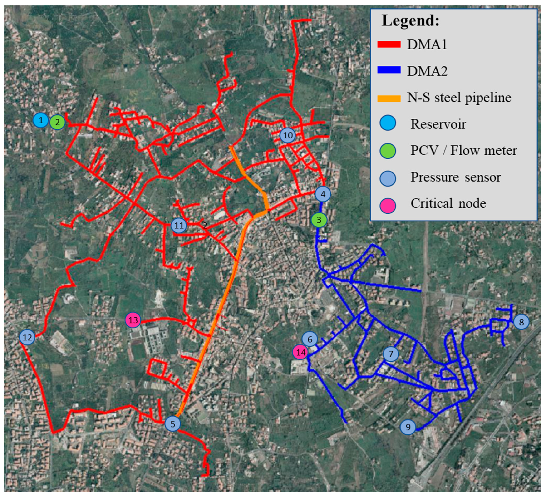
2.1. Case-Study Network

A portion of the municipal WDN of the town of San Giovanni la Punta (Italy) was selected as case-study to evaluate benefits of some rehabilitation and active pressure control strategies.

The WDN (see Figure 1) consists of about 39 km of pipes and supplies about 6100 users (about 2400 households). Two main DMAs were identified in a conjunct work carried out with the water company that manages the water distribution in the network. The two districts supply the northwest area (namely district DMA1, pipes reported in red in Figure 1) and the southeast area (namely district DMA2, pipes reported in blue in Figure 1) of the town.

The whole system is supplied by the reservoir “Alto”, which is located in the northern part of the town at 422 m a.s.l. (maximum capacity approximately equal to 100 m³). The reservoir is supplied by well pumps operated through use of an inverter-based system that adjusts the inlet to maintain a constant water level of 2 m in the reservoir during a period of 24 h. A cast iron conduit conveys flow from the reservoir to the main branches and loops of the WDN including a 2 km long steel pipeline with the function of north–south main distribution line (reported in orange in Figure 1). Most of the pipes larger than DN200 in the WDN are made of steel and cast iron, and date back to the 1980s and 2000s, respectively. Conversely, the small conduits are almost entirely in HDPE and were installed in the early 2000s. Various surveys carried out during the last decade by the water company have revealed the occurrence of leakages in several branches of the WDN. In this regard, a point of weakness of the network concerns the described north–south main distribution line. Indeed, this line is affected by high leakage levels that are the cause of pressure problems (and inadequate water supply) for several households belonging to DMA1.

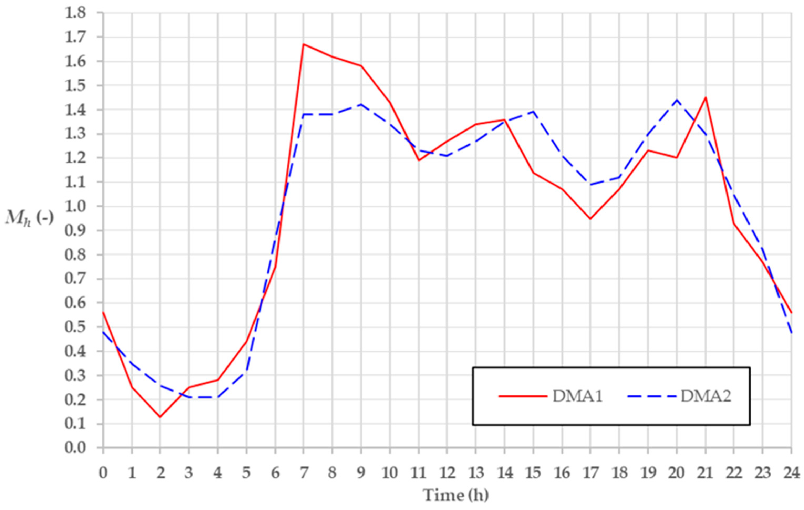
2.2. Monitoring Campaign

A campaign of monitoring was carried out during the research work to explore the behavior of the network in terms of water consumption and pressure in the two districts.

The Specific objective of the experimental monitoring was to identify critical issues in the current operation of the WDN (e.g., identify areas of leakage, hydraulic malfunctioning, etc.). A further objective was to set up a dataset of measurements to be used for the calibration of the simulation model adopted for the analysis of the WDN.

The experimental campaign was carried out separately for the two districts (in the months of October 2018 for DMA2 and April 2019 for DMA1). Installation of pressure sensors and devices required preliminary works aiming at isolation of network sectors and assessment of the condition and settings of existing valves in the network. A flow meter (at the inlet of the district) and five pressure sensors were installed in nodes of each DMA (see Figure 1) for two consecutive weeks. During such periods, flows and pressures were monitored at intervals of 1 and 10 min, respectively. The flow meters used allowed flows to be measured with an accuracy of 0.5%, while pressure sensors provided pressure measurements with 0.1% accuracy. All the data were stored locally and downloaded at the end of the monitoring period for the successive analyses. Recorded measurements enabled determining the daily pattern of the pressure in the two districts, thus, identifying areas at low or high pressure (thus, more or less prone to leakage) in the network during the 24 h. Furthermore, the analysis of the data allowed determining the daily pattern of flows supplied to the two DMAs, thus enabling a measure of the total sum of household consumption and of water leakages in the two districts.

Moreover, the comparison of the data of flow with quarterly data of grouped billed consumption (provided by the water company for each household of the WDN) allowed to unbundle leakage contribution by the total measured flow.

2.3. Model of the Network

A hydraulic model of the network was set up to assess benefits determined by implementation of scenarios of rehabilitation and active pressure control in order to reduce leakage levels in the WDN.

The extended period simulation (EPS) of the WDN was performed, i.e., the simulation was run assuming successive conditions of steady state for 24 h of the day.

Simulations were carried out under the MATLAB environment through the EPANET-MATLAB Toolkit [22]. The toolkit allows exploiting the tools of EPANET software, developed by the EPA (U.S. Environmental Protection Agency) for the simulation of water distribution networks [23]. The adopted skeletonization of the network was taken from the GIS owned by the water utility, which includes not only the primary level of loops but also the secondary one (i.e., the level of pipe branches before the building/household level). Overall, the network was skeletonized using 921 links and 869 nodes. The adopted skeletonization allowed considering a level-wise description of the network (primary and secondary branches and loops) appropriate for the correct allocation of nodal demands consistently with both acquired measurements and available billing data.

Preliminarily, pipe roughness was estimated based on the available information from surveys concerning pipe material and level of pipe corrosion. Notably, the inspection of pipes in different manholes of the network revealed a (high) level of corrosion of the north–south distribution pipeline typical of pipes in operation for several years. Differently, the plastic pipes and those in cast-iron showed better conditions, consistent with their lesser age. The inspection was carried out in about twenty manholes distributed in a rather uniform way in the two DMAs, thus providing an idea of the global conditions of the whole WDN. Roughness values for the three types of pipe materials were properly selected from the literature [24] based on the observed conditions from the field survey.

On this background, values of Hazen–Williams roughness coefficients were set equal to 140, 95, and 75 for pipes in HDPE, cast iron, and old steel, respectively.

Network leakage was evaluated using a pressure-driven approach [25], based on the following equation:

$$Q_k=\beta P_k^{\alpha }{{\displaystyle \sum }}_{J=1}^{n_{j,k}}\frac{L_{j,k}}{2}$$

(1)

where $Q_k$ (L/s) is the leak at the k-node and $P_k$ (m) is the corresponding pressure; n_j,k is the total number of j-pipes converging to node k; $L_{j,k}$ (m) is the length of pipe j converging to node k; and α and β are leakage coefficients to be calibrated.

The analysis of the scientific literature shows efforts to characterize the behavior of leakage in WDNs in terms of values of the leakage exponent α. The value 1.18 has been proposed based on field data [26]. Values ranging between 0.5 and 2.5 have been found depending on pipe material, on the background soil hydraulic characteristics, and on the prominent type of leak [27,28,29,30]. Instead, β has been shown to depend on the level of leakage and on the description of the WDN. Very often, given their large variability, the values of these two coefficients have been chosen in the literature based on the use of specific calibration procedures [31].

A pressure control module was developed in MATLAB. The module was coupled to the hydraulic model to allow the simulation of potential benefits deriving from adoption of active control of pressure in the WDN based on remote RTC [12]. The control module allows implementing architectures of RTC systems and to use various types of PCVs (e.g., screw-based valves; plunger valves, etc.) for pressure control in the WDN. A control strategy (i.e., the sequence of control actions to drive the pressure to the setpoint) derived from the literature [17] was implemented in the module, which assumes that pressure at each of the two DMAs is controlled on the basis of the pressure value in one node (critical node) of the district. Specifically, in the pressure control module, it is assumed that pressure measurements acquired at the critical node are remotely transmitted in real time to the controller that operates the adjustment of the PCV. The control algorithm implemented in the pressure control module provides (at each control time step) the valve shutter displacement $∆a$ (-) based on the deviation $e_t$ (m) at time t between the current pressure value and the related setpoint value at the critical node:

$$∆a=a_{t+∆t_c}-a_t=-K{e}_t,$$

(2)

where $a_t$ and $a_{t+∆t_c}$ are valve opening degrees at time t and $t+∆t_c$, respectively; Δt_c is the control time step, and K (m⁻¹) is the controller gain.

Equation (2) shows that $∆a$ is proportional to $e_t$ through $K$. Therefore, with respect to the shutter position $a$, the adopted algorithm shows the characteristics of an integral-type controller. Moreover, the negative sign in Equation (2) allows considering the negative proportionality between $∆a$ and $e_t$, if gain $K$ is assumed to be intrinsically positive.

Finally, valve regulation is constrained by the limits 0 and 1 (saturation), corresponding to valve fully closed (0) and fully open (1). The control module allows also including limits (of the valve manufacturer) on the mechanical velocity of the shutter of the valve, to prevent risks of unwanted transients in the network [12].

2.4. Model Calibration

The availability of measurements in the network allowed the calibration of the simulation model, thus, increasing the reliability of the simulation results concerning the potential benefits due to implementation of leakage control strategies in the WDN.

Calibration was carried out using the Genetic Algorithm Toolbox available in MATLAB environment. The adopted procedure is based on a recent application [31] and consists in calibrating simultaneously (through a genetic algorithm) the optimal values of the hourly multipliers of the daily curve of consumption and the optimal values of parameters α and β of Equation (1) for leakage evaluation. The values of the leakage parameters were assumed the same for all the network pipes, except for the coefficient β related to the steel north–south steel pipeline that was evaluated separately, to improve model results.

In order to correctly describe the demand dynamics in the network, hourly demand multipliers of each DMA were considered, i.e., coefficients that multiply the average daily consumption and provide the hourly demand in the nodes of the WDN.

Average hourly measured values of flow and pressure, recorded during the monitoring campaign at each DMA, were provided as model input with the aim of identifying the optimal leakage parameters and hourly demand multipliers by minimizing the following objective function:

$$OF={{\displaystyle \sum }}_{h=1}^{n_h}{{\displaystyle \sum }}_{i=1}^{n_i}{\left(\frac{P_{C_{i,h}}-P_{M_{i,h}}}{P_{M_{i,h}}}\right)}^2,$$

(3)

where P_C (m) and P_M (m) are computed and measured pressure values, respectively; n_i is the total number of installed pressure sensors; and n_h is the number of hourly values considered.

Use of Equation (3) was subject to the constraint that total inflow to each DMA is always equal to the sum of household consumption and leakage in the district, at any time step of the simulation.

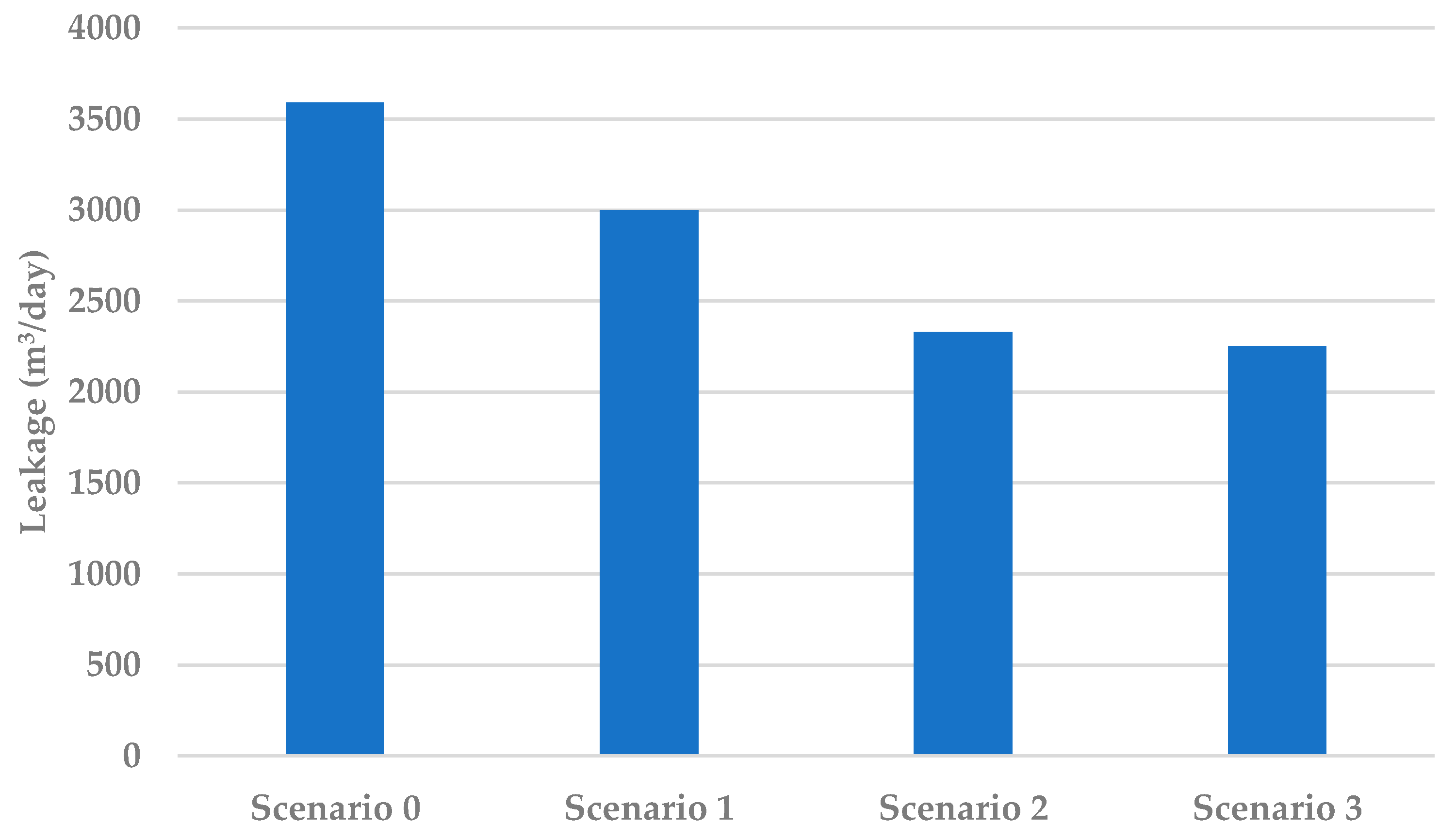
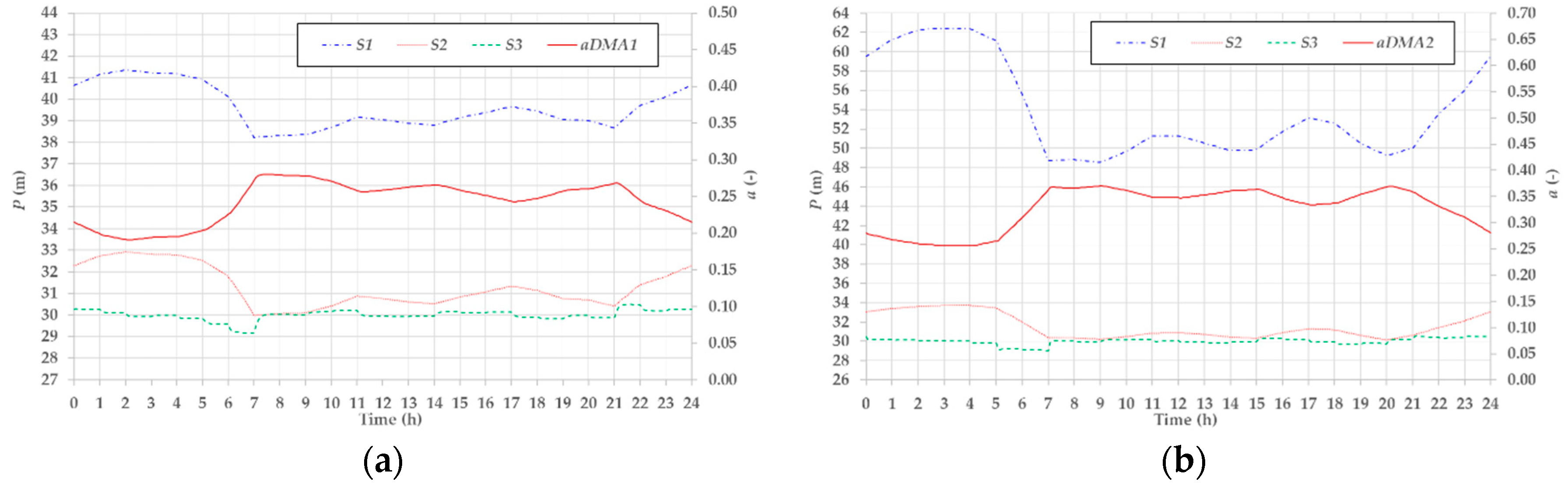
2.5. Scenarios of Simulation

Three main scenarios were considered for the simulations that include options of rehabilitation/active pressure control of the WDN. The first scenario (S1) concerns the rehabilitation of the described north–south steel pipeline in order to eliminate leakages identified during the field surveys. Such scenario includes improvement of water supply to users of DMA1 as determined by the re-arrangement of circulation of flows in the conduits.

The second scenario (S2) adds up to S1 the installation of two PCVs to allow local control of the pressure in the network. The two PCVs are assumed to be conventional screw-based valves and to be installed at the inlet of each DMA (PCV1 at node 2 of the DMA1 and PCV2 at node 3 of the DMA2, as shown in Figure 1). In this scenario, each valve is set with the objective of reducing as much as possible pressure levels in the respective DMA, while ensuring the full demand satisfaction to all the users of the district. This is obtained by preliminarily identifying the critical node of each DMA, that is the node with the lowest value of pressure in the district during 24 h (node 13 for DMA1 and node 14 for DMA2). Then, the scenario considers that pressure at the critical nodes can never drop down below the minimum value of 30 m. Accordingly, the local pressure setpoint at PCV1 and PCV2 outlet was set to 7.5 and 33 m for DMA1 and DMA2, respectively.

The third scenario (S3) considers the adoption of a remote RTC for pressure control in the WDN. Two plunger valves (DN300 for DMA1 and DN80 for DMA2) are assumed to be installed at the same sites as in scenario S2. Recent laboratory experiments have shown this type of valve to provide potential for accurate RTC in WDNs [32]. The scenario assumes the same pressure setpoint (30 m) at the two critical nodes as for scenario S2 (nodes 13 and 14). However, in comparison to scenario S2, the valves are directly controlled on the basis of the remote pressure measurements acquired in real time at the critical nodes. Simulation of scenario S3 included preliminary identification of a suitable value of the controller gain K to perform effective pressure control in the two districts without the occurrence of permanent pressure oscillations [33]. In agreement with previous literature results (e.g., [20,34], the simulations under RTC were carried out using control time $∆t_c$ = 5 min.

Scenarios S1, S2, and S3 were compared to scenario zero (S0), the current reference scenario in which no actions are taken to reduce leakage levels in the network.

3. Results

3.1. Results of the Monitoring Campaign and Leakage Level Estimation

On the one hand, results of the analysis of the data of the monitoring campaign with specific reference to flow measurements at node 2 show that average daily flow to the whole WDN is equal to 56.5 L/s. Moreover, flow measurements at the inlet of DMA2 reveal that average daily inflow to this district is 11.8 L/s. By difference, nodes of DMA1 are supplied with total average daily flow of 44.7 L/s.

On the other hand, the analysis of the billed consumption (from the database of the households) points out consumption for the whole WDN corresponding to an average value of the flow of 14.9 L/s. The same analysis at the scale of DMA, provides 9.9 L/s for DMA1 and 5.0 L/s for DMA2. This last result is consistent with the spatial distribution of population, since about 2/3 of the total population served by the WDN belongs to DMA1.

Based on the above, a comparison of the results of the monitoring campaign and of the billed consumption would confirm a huge level of leakage in the WDN (about 73.6% of the total inflow, i.e., about 92.2 m³/day/km). The same comparison at the scale of DMA shows that leakage levels for DMA1 and DMA2 are equal to 78% (107.4 m³/day/km) and 58% (53.4 m³/day/km), respectively.

3.2. Results of Model Calibration

Figure 2 reports optimal values of the hourly demand multipliers, M_h, for consumption at both DMA1 and DMA2 as a result of the model calibration in the scenario of simulation S0.

The figure shows that the two patterns are rather similar with the occurrence of three main peaks of consumption (the first at early morning, the second at lunch time, and the third at dinner time) as well as with the minimum flow value occurring during the night. Slight differences are shown between the two DMAs with the first peak being larger and in advance for DMA1 as compared to DMA2 due to the widespread presence of commercial activities in DMA1.

Additionally, the calibration returned the optimal values of leakage coefficients of Equation (1). Specifically, the calibration procedure returned α = 0.87 and β = 2.85 × 10⁻⁵. Such values were attributed to both types of pipes, i.e., stainless steel and HDPE. It was not considered the opportunity to differentiate the coefficients for the two types of pipe material given the very modest incidence of pipes in stainless steel as compared to that of pipes in HDPE. As expected, according to the results of the optimization, a larger value of the coefficient was obtained (β = 4.77 × 10⁻⁴) for the north–south steel pipeline.

Results are consistent with previous literature results from similar applications [31,32,33,34,35,36,37], showing values of demand multipliers to range between 0.1 and 1.7, α values close to 1 and β values between 10⁻⁵ and 10⁻⁴.

Values of the absolute mean percent error (MAPE) and of the root mean squared percent error (RMSPE) as obtained by the optimization process for flow and pressure values at the various nodes of installation are shown in

Table 1. Results of model calibration. Values of absolute mean percent error (MAPE) and root mean squared percent error (RMSPE) for flow and pressure.

	DMA1						DMA2
	Flow	Pressure					Flow	Pressure
Node	2	10	11	12	4	5	3	6	7	8	9
MAPE	0.017	0.037	0.040	0.032	0.031	0.022	0.006	0.016	0.014	0.020	0.014
RMSPE	0.020	0.045	0.051	0.038	0.039	0.026	0.008	0.020	0.017	0.025	0.018

for DMA1 and DMA2. Remarkably, the table shows maximum value of MAPE for pressure values to be 4% for DMA1 and 2% for DMA2, while the largest value for the flow is 1.7% as obtained for DMA1. Consistently, maximum RMSPE values obtained for the two DMA are 5.1% and 2.5% at nodes 11 and 8, respectively.

3.3. Results of Simulation Scenarios

Scenarios of intervention described previously in Section 2.5 were simulated in order to evaluate the potential for leakage reduction. The simulations were run with reference to water demands of a “average” day as obtained based on the measured flow discharges during the monitoring campaign. The results of the simulations are summarized in Figure 3.

The figure shows that scenario S1 of rehabilitation of the leaking segments of the north–south steel pipeline allows to reduce total daily leakage volume from about 3600 m³/day to about 3000 m³/day (about 2082 m³/day for DMA1 and 918 m³/day for DMA2). Globally, this would mean recovering about 16.7% (about 6.95 L/s) of the current network leakage. In addition, the rehabilitation of the pipeline leads to improved pressure levels in the WDN, that is reflected into an improved satisfaction of the nodal water demands with specific reference to nodes of DMA1 that were characterized by supply deficit.

As scenario S2 is considered, Figure 3 shows that the total leakage volume in the WDN drops down to 2330 m³/day (1726 m³/day in DMA1 and 604 m³/day in DMA2), that is a 35% leakage reduction with respect to the current scenario S0 (about 14.7 L/s recovered). The figure shows also that replacement of the two PCVs with valves controlled by remote RTC (scenario S3) has further potential to improve the pressure control action with respect to scenario S2. The total leakage volume in the WDN drops down to about 2252 m³/day, that is a 37.5% leakage reduction as compared to S0 (about 15.6 L/s recovered).

Leakage reduction obtained in both scenarios S2 and S3 is strictly depending on the decreasing of the pressure level in the network during the 24 h of the day. The results of local control of the pressure as obtained by using the two PCVs are shown in Figure 4. The figure shows pressure to decrease at the two critical nodes 13 and 14 for DMA1 and DMA2, respectively. However, the desired setpoint of 30 m is achieved only in some hours, while the pressure remains higher than the setpoint for the rest of the day (on average 31.5 and 31.3 m for the two critical nodes). Figure 4 also reports the results of the simulation of scenario S3 with the adoption of remote RTC. The simulation was performed using K = 0.005 m⁻¹ (as obtained by preliminary runs aimed at the tuning of the controller). The figure shows that the used value of the gain allows driving the pressure (at both critical nodes) to the setpoint without incurring in the generation of oscillations of the pressure during the day. Remarkably, the RTC system is able to maintain each pressure setpoint in an accurate way during the 24 h. Specifically, the figure highlights that the maximum pressure deviation from the setpoint is smaller than 1 m at both DMAs (against 3–4 m in the case of local control of S2). Figure 4 also reports the curve of the valve opening settings aDMA1 and aDMA2 in the two districts. As shown, openings/closures of the valve shutter are consistent with the daily water demand pattern at the two DMAs. In fact, the two plunger valves are adjusted by the control algorithm in order to close majorly during night hours (when pressure levels are normally higher) and to open during the peaks of the water demand.

As already discussed, the simulations under EPS were performed considering a day with average characteristics among the days of the monitoring campaign. However, it should be stressed that benefits of remote RTC as compared to local control of pressure are normally emphasized under conditions of high spatiotemporal variability of water demands in the WDN. In fact, while local control remains affected by uncertainty in water demands, in principle, remote RTC systems are able to assure appropriate pressure control in real time in all the circumstances.

An important aspect that deserves discussion concerns the concurrent use of the two PCVs installed at the two DMAs. In fact, PCV2 significantly reduces pressure levels at DMA2 while sustaining pressure in the upstream DMA1, thus reducing beneficial effects of pressure reduction as determined by PCV1. In this regard, the results of a further simulation (not presented here) of the WDN that includes implementation of PCV1 only, allowed quantifying that the pressure value at node 4 (upstream of PCV2) would be about 4 m less than the pressure value determined at the same node in scenario S2.

The accuracy (thus the transferability into practice) of the simulation results obtained deserves specific discussion. The availability of measurements from the monitoring campaign allowed appropriate calibration of the simulation model, with the average MAPE (Table 1) corresponding to absolute error in pressure in the order of 0.5 m (for a 30 m setpoint). Based on the results of the simulations, such an error is generally smaller than pressure differences as obtained by the comparison of the different scenarios, thus, confirming the reliability of the results of leakage reduction.

Finally, it should be stressed that, although strategies of active pressure control such as those discussed in this paper may help reducing leakage levels in WDNs, they can also be a cause of reduction of the network resilience during emergency conditions (e.g., firefighting scenarios). However, strategies of remote RTC may allow performing a real-time adjustment of the pressure control valves in the network, according to the requirements, preventing water hammer conditions and restoring appropriate levels of pressure in the WDN to cope with the emergency.

4. Conclusions

A simulation analysis was carried out to evaluate the potential of rehabilitation measures and active pressure control strategies for leakage reduction in a WDN in southern Italy.

Three main scenarios were considered for the simulations. The first scenario (S1) concerned the rehabilitation of a steel pipeline of the WDN in order to eliminate leakages that were identified during the survey of the network. The second scenario (S2) added to S1 the installation of two PCVs to allow local control of the pressure in the network. The third scenario (S3) considered the adoption of a remote RTC for pressure control in the WDN by means of two plunger valves in place of the PCVs adopted in S2. The three scenarios were compared to scenario zero (S0), i.e., the current reference scenario in which no actions are taken to reduce leakage levels in the network.

The analysis has shown that a combination of the used strategies can significantly improve the network performance. Specifically, rehabilitation of the steel pipeline (scenario S1) would provide a significant reduction of the current leakage level of the WDN. Addition of local pressure control (scenario S2) would add further benefits. The adoption of remote RTC (scenario S3) in comparison with local pressure control increases leakage reduction. Additional benefits of remote RTC as compared to local control of PCVs would be observed under conditions of high spatiotemporal variability of water demands in the WDN.

Two main aspects played an important role in corroborating the reliability of the results of the analysis. Firstly, simulations were based on the results of the accurate calibration of model parameters relying on a program of measurements carried out during the monitoring campaign. Secondly, the modeling of the pressure control processes by using local control of PCVs and remote RTC was carried out based on the literature results of consolidated experimental investigations.

Evidently, the results of this analysis must be considered as preliminary and open to further research work. Transferability of the obtained results requires testing the methodology on other WDNs with different hydraulic characteristics and topology. In addition, in real cases, the choice of measures of intervention to adopt would require the evaluation of the benefit in terms of leakage reduction, but cannot prescind also a comprehensive analysis of the costs (including economic, environmental, and social costs) of each scenario of implementation.

References

1. Berardi, L.; Laucelli, D.B.; Simone, A.; Mazzolani, G.; Giustolisi, O. Active Leakage Control with WDNetXL. Procedia Eng. 2016, 154, 62–70. [Google Scholar] [CrossRef] [Green Version]
2. Wu, Z.Y.; Sage, P.; Turtle, D. Pressure-Dependent Leak Detection Model and Its Application to a District Water System. J. Water Resour. Plan. Manag. 2010, 136, 116–128. [Google Scholar] [CrossRef]
3. Romano, M.; Kapelan, Z.; Savic, D. Geostatistical techniques for approximate location of pipe burst events in water distribution systems. J. Hydroinform. 2013, 15, 634–651. [Google Scholar] [CrossRef]
4. Berardi, L.; Giustolisi, O.; Kapelan, Z.; Savic, D. Development of pipe deterioration models for water distribution systems using EPR. J. Hydroinform. 2008, 10, 113–126. [Google Scholar] [CrossRef] [Green Version]
5. Thornton, J. Water Loss Control Manual; McGraw Hill Professional: New York, NY, USA, 2002. [Google Scholar]
6. Ciaponi, C.; Franchioli, L.; Murari, E.; Papiri, S. Procedure for Defining a Pressure-Outflow Relationship Regarding Indoor Demands in Pressure-Driven Analysis of Water Distribution Networks. Water Resour. Manag. 2015, 29, 817–832. [Google Scholar] [CrossRef]
7. Le Gat, Y.; Eisenbeis, P. Using maintenance records to forecast failures in water networks. Urban Water 2000, 2, 173–181. [Google Scholar] [CrossRef]
8. Prescott, S.L.; Ulanicki, B. Improved Control of Pressure Reducing Valves in Water Distribution Networks. J. Hydraul. Eng. 2008, 134, 56–65. [Google Scholar] [CrossRef]
9. Nicolini, M.; Zovatto, L. Optimal Location and Control of Pressure Reducing Valves in Water Networks. J. Water Resour. Plan. Manag. 2009, 135, 178–187. [Google Scholar] [CrossRef]
10. Pezzinga, G.; Gueli, R. Discussion of “Optimal Location of Control Valves in Pipe Networks by Genetic Algorithm” by LFR Reis, RM Porto, and FH Chaudhry. J. Water Resour. Plan. Manag. 1999, 125, 65–67. [Google Scholar] [CrossRef]
11. Creaco, E.; Pezzinga, G. Comparison of Algorithms for the Optimal Location of Control Valves for Leakage Reduction in WDNs. Water 2018, 10, 466. [Google Scholar] [CrossRef] [Green Version]
12. Campisano, A.; Modica, C.; Reitano, S.; Ugarelli, R.; Bagherian, S. Field-Oriented Methodology for Real-Time Pressure Control to Reduce Leakage in Water Distribution Networks. J. Water Resour. Plan. Manag. 2016, 142, 04016057. [Google Scholar] [CrossRef]
13. Berardi, L.; Simone, A.; Laucelli, D.B.; Ugarelli, R.M.; Giustolisi, O. Relevance of hydraulic modelling in planning and operating real-time pressure control: Case of Oppegård municipality. J. Hydroinform. 2018, 20, 535–550. [Google Scholar] [CrossRef] [Green Version]
14. Page, P.R.; Abu-Mahfouz, A.M.; Mothetha, M.L. Pressure Management of Water Distribution Systems via the Remote Real-Time Control of Variable Speed Pumps. J. Water Resour. Plan. Manag. 2017, 143, 04017045. [Google Scholar] [CrossRef] [Green Version]
15. Creaco, E.; Walski, T. Operation and Cost-Effectiveness of Local and Remote RTC. J. Water Resour. Plan. Manag. 2018, 144, 04018068. [Google Scholar] [CrossRef]
16. Campisano, A.; Schilling, W.; Modica, C. Regulators’ setup with application to the Roma–Cecchignola combined sewer system. Urban Water 2000, 2, 235–242. [Google Scholar] [CrossRef]
17. Campisano, A.; Creaco, E.; Modica, C. RTC of Valves for Leakage Reduction in Water Supply Networks. J. Water Resour. Plan. Manag. 2010, 136, 138–141. [Google Scholar] [CrossRef]
18. Giustolisi, O.; Ugarelli, R.M.; Berardi, L.; Laucelli, D.B.; Simone, A. Strategies for the electric regulation of pressure control valves. J. Hydroinform. 2017, 19, 621–639. [Google Scholar] [CrossRef] [Green Version]
19. Bakker, M.; Rajewicz, T.; Kien, H.; Vreeburg, J.H.G.; Rietveld, L. Advanced control of a water supply system: A case study. Water Pr. Technol. 2014, 9, 264–276. [Google Scholar] [CrossRef] [Green Version]
20. Page, P.R.; Abu-Mahfouz, A.M.; Yoyo, S. Parameter-Less Remote Real-Time Control for the Adjustment of Pressure in Water Distribution Systems. J. Water Resour. Plan. Manag. 2017, 143, 04017050. [Google Scholar] [CrossRef] [Green Version]
21. Creaco, E.; Campisano, A.; Modica, C. Testing behavior and effects of PRVs and RTC valves during hydrant activation scenarios. Urban Water J. 2018, 15, 218–226. [Google Scholar] [CrossRef]
22. Eliades, D.G.; Kyriakou, M.; Vrachimis, S.; Polycarpou, M.M. EPANET-MATLAB toolkit: An open-source software for interfacing EPANET with MATLAB. In Proceedings of the 14th International Conference on Computing and Control for the Water Industry (CCWI 2016), Amsterdam, The Netherland, 1–4 November 2016. [Google Scholar]
23. Rossman, L.A. EPANET 2: Users Manual; National Risk Management Research Laboratory: Cincinnati, OH, USA, 2000. [Google Scholar]
24. Williams, G.S.; Hazen, A. Hydraulic Tables: The Elements of Gagings and the Friction of Water Flowing in Pipes, Aqueducts, Sewers, etc. as Determined by the Hazen and Williams Formula and the Flow of Water Over Sharp-Edged and Irregular Weirs, and the Quantity Discharged, as Determined by Bazin’s Formula and Experimental Investigations Upon Large Models; J. Wiley & Sons: Hoboken, NJ, USA, 1908. [Google Scholar]
25. Germanopoulos, G. A technical note on the inclusion of pressure dependent demand and leakage terms in water supply network models. Civ. Eng. Syst. 1985, 2, 171–179. [Google Scholar] [CrossRef]
26. Goodwin, S.J. The Results of the Experimental Programme on Leakage and Leakage Control; WRC Environmental Protection: Swindon, UK, 1980. [Google Scholar]
27. Greyvenstein, B.; Van Zyl, J.E. An experimental investigation into the pressure—leakage relationship of some failed water pipes. J. Water Supply Res. Technol. 2007, 56, 117–124. [Google Scholar] [CrossRef]
28. Farley, M.; Trow, S. Losses in Water Distribution Networks: A Practitioners’ Guide to Assessment, Monitoring and Control. Water Intell. Online 2015, 4. [Google Scholar] [CrossRef]
29. Al-Ghamdi, A.S. Leakage–pressure relationship and leakage detection in intermittent water distribution systems. J. Water Supply Res. Technol. 2011, 60, 178–183. [Google Scholar] [CrossRef]
30. Ferrante, M. Experimental Investigation of the Effects of Pipe Material on the Leak Head-Discharge Relationship. J. Hydraul. Eng. 2012, 138, 736–743. [Google Scholar] [CrossRef]
31. Di Nardo, A.; Di Natale, M.; Gisonni, C.; Iervolino, M. A genetic algorithm for demand pattern and leakage estimation in a water distribution network. J. Water Supply Res. Technol. 2015, 64, 35–46. [Google Scholar] [CrossRef]
32. Campisano, A.; Modica, C.; Musmeci, F.; Bosco, C.; Gullotta, A. Laboratory experiments and simulation analysis to evaluate the application potential of pressure remote RTC in water distributions networks. Water Res. 2020, 183, 116072. [Google Scholar] [CrossRef] [PubMed]
33. Ziegler, J.G.; Nichols, N.B. Optimum Settings for Automatic Controllers. J. Dyn. Syst. Meas. Control. 1942, 115, 220–222. [Google Scholar] [CrossRef]
34. Creaco, E.; Franchini, M. A new algorithm for real-time pressure control in water distribution networks. Water Supply 2013, 13, 875–882. [Google Scholar] [CrossRef]
35. Letting, L.; Hamam, Y.; Abu-Mahfouz, A.M. Estimation of Water Demand in Water Distribution Systems Using Particle Swarm Optimization. Water 2017, 9, 593. [Google Scholar] [CrossRef] [Green Version]
36. Tucciarelli, T.; Criminisi, A.; Termini, D. Leak Analysis in Pipeline Systems by Means of Optimal Valve Regulation. J. Hydraul. Eng. 1999, 125, 277–285. [Google Scholar] [CrossRef]
37. Maskit, M.; Ostfeld, A. Leakage Calibration of Water Distribution Networks. Procedia Eng. 2014, 89, 664–671. [Google Scholar] [CrossRef] [Green Version]
Figure 1. Sketch of the water distribution network (WDN) with identification of significant nodes (with critical nodes in magenta), districts district metered area 1 (DMA1) (in red) and DMA2 (in blue), and north–south main distribution line (in orange).
Water 12 02215 g001
Figure 2. Results of model calibration. Hourly demand multipliers for the two DMAs.
Water 12 02215 g002
Figure 3. Potential leakage reduction under implementation of the different scenarios.
Water 12 02215 g003
Figure 4. Pressure levels at the critical nodes of (a) DMA1, and (b) DMA2 under scenarios S1, S2, S3.
Water 12 02215 g004