Assessment of Surface Water Quality Using Multivariate Analysis: Case Study of the Crati River, Italy

Abstract

The water vulnerability of the Crati river (Calabria, Italy), was assessed by applying chemometric methods on a large number of analytical parameters. This study was applied to a data set collected in the years 2015–2016, recording 30 physical–chemical and geological parameters at 25 sampling points, measured both for water and for sediments. The processing of the data by principal component analysis (PCA) allowed for highlighting the influence of the components most responsible for pollution. The accumulation of heavy metals in the water was detected only in two samples near the source of the river. On the contrary, their concentration values in the sediments exceeded the legal limit in several sites, probably due to their proximity to urban areas. In this case, high concentrations of chromium, mercury and nickel were detected both at the mouth of the river and along the valley. Lead was only detected in one sediment sample. The multivariate analysis techniques proved to be very useful to completely characterize the areas surrounding a river course and facilitate the development of a risk map to monitor health risks to the local population.

1. Introduction

Environmental stability is often modified by man to meet his needs, but in many cases, this behavior involves the pollution of air, water and soil with a deterioration in the quality of life. The quality of surface waters is a useful indication of the status of a territory, reflecting the effects of human activities on natural ecosystems [1]. Urbanization, industries, land use, modern agricultural practices and animal husbandry, alone or in synergy, can affect aquatic ecosystems and, if these alterations are not limited, the natural balance of ecosystems can be irreversibly compromised.

In order to minimize the negative impact of human activities on aquatic systems, the development of rapid and reliable systems for monitoring water quality is a research priority in this field [2]. The main target for assessing the environmental status of rivers, lakes, groundwater and coastal waters is the regular detection of water pollutants and the causes of their presence [3,4].

The absence or inadequate treatment of urban waste water causes the release of organic substances, bacteria and compounds containing nitrogen or phosphorus into sewers and, in turn, into rivers [5]. This negligence, together with the waste of industrial and agricultural activities, are the main sources of water pollution, with significant repercussions on the health of plants, animals and humans.

In the present study, many physical–chemical and geological parameters were recorded during a monitoring program from September 2015 to March 2016 on the waters of the Crati River and its main tributaries, in order to prepare a risk map of the of the study area [6].

In recent years, the development of new analytical methodologies has allowed for the processing of physical and chemical data at a speed unthinkable a few decades ago and has made it possible to solve complex analytical systems through multivariate analysis, which allows for the simultaneous use of all the variables involved. Statistical information for each variable is extracted from the collected experimental data, identifying the correlations between the variables or any outlier data. In most cases, a mathematical model is built that predicts the quantitative values of a variable (the response) from the values of a set of variables (the predictors) measured for known samples. Such methods are called regression methods. In a second phase, the model can undergo an optimization process, in which the number of variables or samples can be modified and the data that appear discordant with the rest (outliers) are eliminated. This model must necessarily be subjected to a validation process, consisting of a series of statistical and applicative tests to ascertain the effectiveness of the model in predicting new samples with unknown composition.

In this work, chemometric techniques have been applied to data matrices in order to develop a multivariate model capable of correlating environmental conditions with health and quality of life [7,8,9,10,11,12,13,14,15,16]. Data processing was performed using dedicated software, capable of managing the complexity of the system and simultaneously assessing the impact of single analytical parameters. Multivariate analysis was able to select and consider the parameters containing the most representative information, thus providing a highly reliable response on the quality of the water and the surrounding environment [17,18,19]. The results of this investigation can be very useful for developing a risk map of the studied area as an important reference document for potential epidemiological studies.

2. Materials and Methods

2.1. Study Area

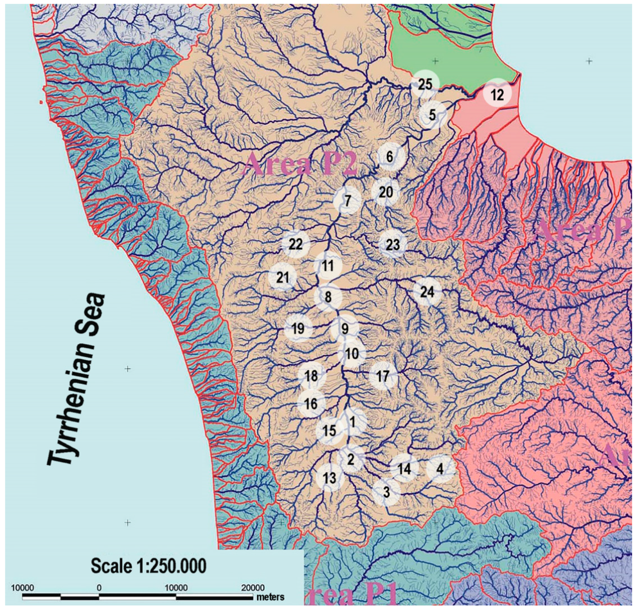
The Crati River is in Calabria, a region of south of Italy. The studied area is bounded by a watershed from the Tyrrhenian Sea to the Ionian Sea (CS) toward the south and by that of the rivers Noce, Lao, Crati and other small basins toward the north. The territory is situated between the Tyrrhenian coast and the peak of Coccovello mountain and extends to the other mountain peaks of Rocca Rossa, Murgia del Principe, Sirino and Zaccana, up to the Grattaculo. The area reaches the Pollino promontory where Dolcedorme (2271 m above sea level) reaches the highest peak in the area, followed by the peaks of Timpone Rotondella and Timpone Neviera and finally descends to the Ionian coast. This area is completely surrounded by the sea.

The studied region shows the predominantly mountainous orographic configuration with a very harsh mountain range, often with deep valleys and steep slopes. In the south of the region, the upland Sila has a considerable extension and is characterized by large shelves of around 1300 m, including the most important peaks of Botte Donato (1929 m above sea level), Montenero (1881 m), Volpintesta (1730 m) and Gariglione (1785 m).

2.2. Sampling

The monitored sites were included in the geographic information system, WGS84 World Geodetic System 1984, which describes the main characteristics of the water: name, basin code and geographic coordinates [20,21]. According to this georeferencing system, the Italian territory is located in zone 33 N (12° to 18° equator parallels).

Table 1. Georeferencing of the sampling points.

n	Site	Sampling Point	Territory	WGS84 33N North	WGS84 33N East
1	River Head	Crati River 13	Zumpano	4353248	608714
2		Crati River 15	Cosenza	4349227	609404
3		Crati River 16	Aprigliano	4344566	614193
4		Crati River 17	Aprigliano	4346446	621277
5	Mouth of river	Crati River 1	Corigliano Calabro	4392908	620350
6		Crati River 2	Terranova di Sibari	4386956	614668
7		Crati River 3	Santa Sofia d’Epiro	4382060	607969
8	Downstream of purifiers	Crati River 4	Bisignano	4368764	605805
9		Crati River 7	Lattarico/Montalto Uffugo	4364667	607776
10		Crati River 8	Luzzi/Montalto Uffugo	4362207	608213
11		Crati River 9	Rende	4373900	605149
12		Crati River 10	Corigliano Calabro	4396715	628213
13	Tributaries	Busento River	Cosenza	4346356	606441
14		Cardone Torrent	Cosenza	4347897	616037
15		Campagnano River	Rende	4352384	606533
16		Emoli Torrent	Rende	4355775	604189
17		Arente Torrent	Castiglione Cosentino	4359164	613541
18		Settimo River	Montalto Uffugo	4359369	604367
19		Annea Torrent	Montalto Uffugo	4365519	602364
20		Galatrella Torrent	Terranova di Sibari	4382782	613773
21		Finita Torrent	Lattarico	4372149	600294
22		Turbolo Torrent	Mongrassano	4376036	602243
23		Duglia Torrent	Mongrassano	4375974	614532
24		Mucone River	Bisignano	4370307	619125
25		Coscile River	Sibari	4396816	618629

lists the east and north geographic coordinates of the sampling sites monitored in this study.

The sampling sites were distributed along the Crati River as follows: four at the river head (samples Crati13, Crati15, Crati16, Crati17), seven located downstream of the purifier (samples Crati2, Crati3, Crati4, Crati7, Crati8, Crati9, Crati10) and 14 at the mouth of the river (samples Crati1, Busento, Cardone, Campagnano, Emoli, Arente, Settimo, Annea, Galatrella, Finita, Turbolo, Duglia, Mucone, Coscile). These sampling sites correspond to the long-term monitoring sites of the Regional Agency for the Environment of Calabria and were therefore selected according to the protocol detailed in the Dlsg N. 60/2000 [22]. The geographical area and the sampling sites are reported in Figure 1.

The data were collected from September 2015 to July 2016. Sampling was carried out according to Italian standards [23]. All water samples were collected in sterile plastic and glass bottles for the analysis of inorganic and organic compounds, respectively, and stored at 4 °C until analysis. These samples were analyzed without treatment. The sediment sampling was carried out at points located far from drains and the riverside by means of a cylindrical core, drilling to a depth of about 10 cm by vertical sinking. Each sediment surface sample weighing 1 kg was sealed in a transparent plastic bag to minimize sample contamination [24]. The sediment samples, still wet, were weighed, homogenized and transferred to a glass container. Subsequently, the samples were dried in a stove at a constant temperature of 105 °C until a constant weight, which was recorded as dry weight. Finally, the samples were ground by crushing any agglomerates and sieved through a 2-mm net. For the measurement of radioactivity, the sediment samples were placed in a 1000 mL Marinelli beaker.

Thirty analytical parameters were recorded for each sample, according to the Italian and European protocols [23,24,25,26,27,28,29,30]: pH, temperature, flow velocity, electrical conductivity, dissolved oxygen, total nitrogen (total N), nitric nitrogen (NO₃⁻), nitrous nitrogen (NO₂⁻), ammonium ion (NH₄⁺), total phosphorus (total P), cadmium (Cd), iron (total Fe), chrome (Cr), nickel (Ni), lead (Pb), boron (B), aluminum (Al), arsenic (As), selenium (Se), zinc (Zn), copper (Cu), mercury (Hg), pesticides (e.g., alachlor, atrazine, aldrin, heptachlor, hexachlorobenzene, endosulfan, methoxychlor) and gamma radiation. The determination of pH, temperature, flow velocity, electrical conductivity and dissolved oxygen was performed in situ using multiparameter probes. The concentration of pesticides and heavy metals and the measurement of radioactivity were performed within 48 h of sampling.

The analytical parameters were averages of six determinations. All the relative standard deviation values fell within the range 1.16–5.03%, demonstrating both the low uncertainty and the robustness of the analytical methods applied.

2.3. Instruments and Software

Analytical determinations were carried out at the Physics Laboratory and Water Unit of the Regional Environment Agency of Calabria, Department of Cosenza, Italy. The concentration of pesticides was determined by GC-MS using the Agilent 5975C GC system coupled with the Agilent 5973 MS detector. The concentration of heavy metals was performed by the Shimadzu UV-160 atomic absorption spectrophotometer at a wavelength of 220 and 882 nm in a 1-cm quartz cell and by an Agilent 7500 to carry out inductively coupled plasma spectrometry using argon gas.

The Unscrambler X 10.5^® software package (Camo Process As., Oslo, Norway), equipped with several statistical packages, supported the application of multivariate algorithms. It also allowed for the optimization of the calibration models and the development of validation procedures.

2.4. Multivariate Analysis

The application of chemometric techniques is very useful for describing many variables in an analytical system and to define possible relationships between them. Principal Component Analysis (PCA) is one of the most important data reduction methods for a multivariate data set [17,18,19]. It is characterized by the ability to reduce the dimensionality of a data matrix, while retaining most of the original information. A linear combination is applied to transform the original variables (X) into a limited number of new principal components (PCs)

X = t₁p₁^′ + t₂p₂^′ +…+ t_Ap_A^′ + E

(1)

where t_n are the score values, p_n are the loading values and E is the residual matrix.

This chemometric approach defines the minimum number of PCs capable of describing the total sum of the data matrix square. The object classes are defined by scores and loadings. The scores contain all the information concerning the objects (experiment, sample, etc.) and correspond to their projection in the space of the principal components. The loadings are instead the projections of the variables (x, y and z) in the PC space.

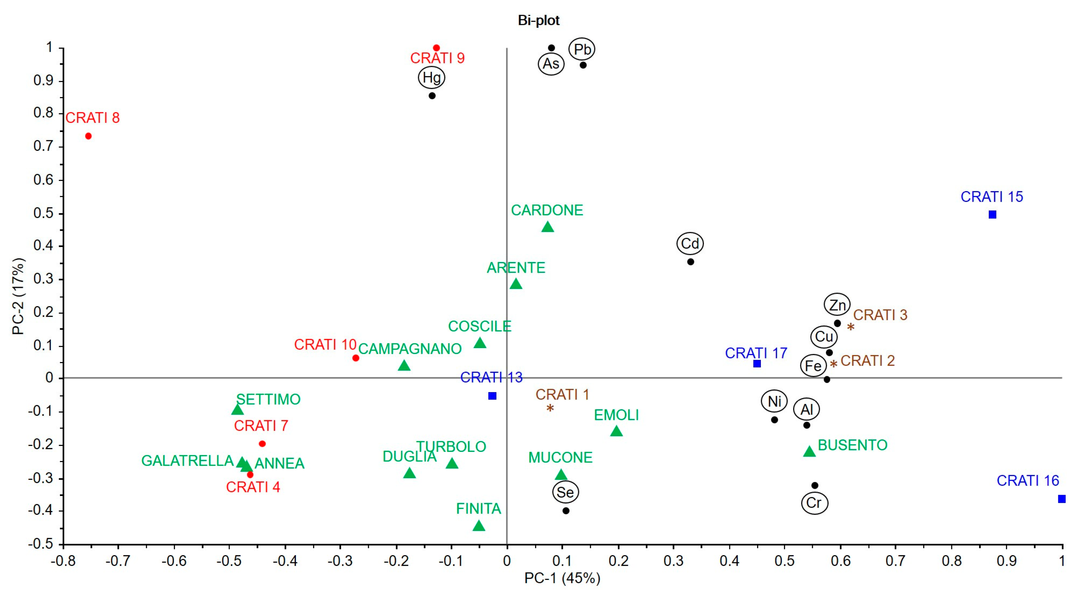
Scores and loadings can be represented on a bi-plot. This is a two-dimensional scatter plot or a score map for two specific components (PCs), with the X-loadings displayed on the same plot. It enables the simultaneous interpretation of sample properties and variable relationships.

2.5. Data Sets

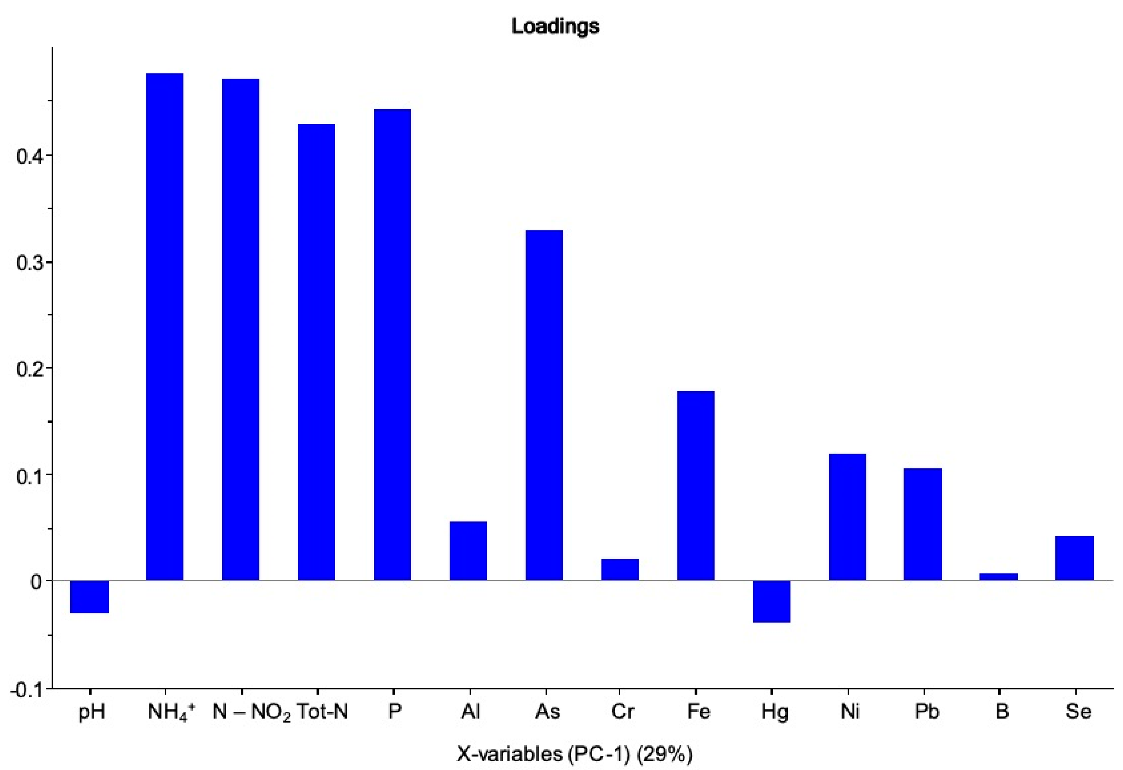
Two data sets were built, respectively, for water and sediment samples. Each set was built using 30 analytical parameters per site, for a total of 750 values. Firstly, a selection of the variables carrying the most useful information was made. This selection represents a critical step that must be carefully considered, because the exclusion of important variables can lead to misleading results in building the model. The amount of relevant information does not necessarily increase when multiple variables are included, indeed, random noise may even increase. Figure 2 shows the bar plot of the loadings, describing the different contributions of each variable in building the principal components. The importance of the different variables for the components is here evident.

The variance value was adopted as a discriminating criterion for selecting the parameters, discarding those showing a relative standard deviation (RSD) value of less than 10%. The raw data were normalized before applying PCA by using the weighted standard deviation procedure, in order to balance the weight of each value measured on different scales on a common scale.

Table 2. Data set including the analytical parameters measured for the water samples. The concentration values are expressed as μg/mL. Measured values higher than those allowed by the reference standard are shown in bold.

Samples	pH	NH₄⁺	N-NO2	N Total	Total P	Al3+	As	Cr	Fe Total	Hg	Ni	Pb2+	B	Se
Crati 13	8.0	0.19	0.06	1.37	163	0.9	0.09	0.4	36	0.3	0.5	3.0	5.0	0.04
Crati 15	8.1	0.19	0.08	1.64	191	0.9	0.09	0.4	43	0.09	0.4	5.0	5.0	0.04
Crati 16	7.5	0.19	0.06	0.49	77	0.9	0.8	0.4	12	0.09	0.9	0.4	10.0	0.04
Crati 17	7.2	0.19	0.009	0.31	8	25.0	0.09	0.4	34	0.09	0.4	0.4	1.0	0.04
Crati 1	8.1	0.40	0.03	2.50	55	0.9	0.4	2.0	2.0	0.10	2.0	0.4	21.0	0.20
Crati 2	7.8	0.50	0.03	2.10	59	0.9	0.4	1.0	0.6	0.10	1.0	0.4	20.0	0.20
Crati 3	7.3	0.60	0.03	2.10	90	0.9	0.5	2.0	10	0.09	2.0	0.4	50.0	0.20
Crati 4	7.8	2.00	0.09	3.60	148	0.9	0.6	1.0	80	0.09	2.0	3.0	0.0	0.10
Crati 7	7.8	5.50	0.20	6.78	250	0.9	1.0	1.0	49	0.09	0.9	2.0	0.0	0.20
Crati 8	7.5	2.60	0.15	1.30	301	5.0	0.7	1.0	65	0.09	21.0	2.0	0.0	0.10
Crati 9	7.6	4.00	0.20	5.28	306	14.0	0.8	0.4	39	0.09	0.4	3.0	41.0	0.04
Crati 10	8.0	2.80	0.10	3.84	284	0.9	0.6	1.0	48	0.09	1.0	3.0	0.0	0.20
Busento	8.3	0.20	0.10	1.58	121	0.9	0.09	0.4	39	0.09	0.4	6.0	10.0	0.04
Cardone	7.5	0.19	0.09	1.26	128	0.9	0.5	0.4	38	0.09	0.5	4.0	19.0	0.10
Campagnano	8.3	0.19	0.009	0.29	80	0.9	0.09	0.4	7.0	0.09	9.0	0.4	3.0	0.04
Emoli	8.0	0.19	0.02	0.82	38	0.9	0.4	0.5	37	0.09	0.4	4.0	5.0	0.04
Arente	6.5	0.19	0.009	0.83	17	0.9	0.4	0.4	41	0.09	0.4	3.0	14.0	0.10
Settimo	8.0	0.19	0.009	0.72	50	0.9	0.7	0.4	22	0.09	0.9	2.0	0.0	0.20
Annea	7.7	0.19	0.05	0.17	60	0.9	0.5	0.4	55	0.09	0.9	4.0	45.0	0.04
Galatrella	8.4	0.20	0.01	1.20	62	0.9	0.09	0.5	36	0.09	2.0	3.0	0.0	0.20
Finita	8.1	0.20	0.009	0.70	20	0.9	0.09	1.0	36	0.09	1.0	3.0	0.0	0.04
Turbolo	7.9	0.70	0.01	1.61	32	0.9	0.4	2.0	0.4	0.09	2.0	0.4	42.0	0.30
Duglia	7.5	0.60	0.02	1.40	120	0.9	0.09	0.4	116	0.09	1.0	0.4	0.0	0.10
Mucone	7.4	0.19	0.009	0.90	111	3.0	0.09	0.4	45	0.09	0.4	0.4	0.0	0.10
Coscile	8.1	0.60	0.01	1.81	35	0.9	0.5	2	0.4	0.09	2.0	0.4	20.0	0.04

and

Table 3. Data set including the analytical parameters calculated for the sediment samples. The concentration values are expressed as mg/mL. Measured values higher than those allowed by the reference standard are shown in bold.

Samples	Al3+	As	Cd Total	Cr	Fe Total	Hg	Ni	Pb2+	Se	Cu	Zn
Crati 13	20123	2.3	0.09	33.2	22962	0.04	18.9	10.8	0.09	14.3	53.7
Crati 15	24450	2.6	0.20	49.0	28694	0.05	24.6	26.3	0.10	25.3	116.4
Crati 16	29266	1.3	0.10	71.1	46164	0.04	33.9	8.8	0.20	25.1	95.5
Crati 17	27787	4.4	0.09	62.1	29285	0.04	32.3	4.6	0.00	15.3	67.5
Crati 1	24714	2.5	0.09	41.2	24831	0.04	20.2	7.3	0.09	13.8	61.5
Crati 2	29927	3.5	0.10	54.4	31342	0.04	26.8	11.7	0.10	20.8	80.8
Crati 3	31502	3.5	0.10	56.2	30765	0.06	28.2	12.7	0.10	21.2	82.4
Crati 4	12667	0.6	0.09	26.1	13150	0.04	12.7	3.5	0.09	10.5	34.3
Crati 7	13158	1.1	0.09	21.9	16102	0.04	12.6	5.6	0.09	8.5	41.3
Crati 8	8240	5.0	0.09	13.4	13965	0.12	8.1	4.7	0.09	5.1	26.8
Crati 9	14520	5.0	0.09	21.3	18970	0..06	14.8	59	0.10	16.5	48.7
Crati 10	17580	2.4	0.09	27.1	18720	0.06	17.1	8.1	0.09	9.4	45.3
Busento	19106	1.5	0.10	43.6	28096	0.04	33.9	8.8	0.20	25.1	95.5
Cardone	21103	2.3	0.10	35.9	28632	0.10	19.9	20.3	0.09	13.5	62.9
Campagnano	12629	1.3	0.09	18.6	13470	0.07	37.3	8.7	0.09	11.5	61.5
Emoli	26361	2.4	0.09	57.8	21083	0.05	29.8	5.9	0.09	13.9	45.8
Arente	19563	4.9	0.09	18.6	25699	0.04	22.6	12.1	0.10	16.7	55.3
Settimo	13961	2.2	0.09	23.1	16141	0.04	12.2	5.5	0.09	5.9	34.0
Annea	12141	1.1	0.09	27.2	16146	0.04	16.1	3.6	0.09	4.9	33.6
Galatrella	9282	0.9	0.09	29.0	12524	0.04	16.8	3.8	0.09	11.7	25.6
Finita	20112	1.7	0.09	38.1	17499	0.04	17.2	6.0	0.40	12.9	50.5
Turbolo	13720	1.3	0.09	37.1	18347	0.04	23.0	2.9	0.09	19.8	38.1
Cocchiato	14533	2.3	0.09	21.3	13354	0.04	9.6	4.9	0.10	7.3	37.3
Duglia	23902	0.7	0.09	31.1	22854	0.04	11.8	6.1	0.09	10.3	42.6
Mucone	26918	0.9	0.10	42.1	27165	0.04	16.3	5.2	0.09	13.1	51.6
Coscile	17438	2.9	0.09	38.0	20571	0.06	23.6	9.3	0.09	12.8	55.6

list the values of the selected parameters (means of six measurements) from the analysis of water and sediment samples, respectively.

3. Results

The PCA multivariate approach was applied to the data sets, considering the sampling sites as objects and the measured parameters as variables. The algorithm decomposed the original variables into main components (PCs). Then, the original input matrix (matrix X) was transformed into the matrix of the multivariate model. This matrix consisted of two new matrices represented by the scores, containing all the information concerning the objects (experiment, sample, etc.) and the loadings, which were the projection of the variables (x, y and z) in the PC space.

Figure 3 and Figure 4 show the bi-plot graphs, which respectively represent scores and loadings for the water and sediment samples. The graphs show how the sampling sites could be grouped according to the variables considered.

4. Discussion

The bi-plots reported in Figure 3 and Figure 4 enable the identification of the main characteristics of the sampling points through a simultaneous evaluation of the chemical–physical parameters. This allows for a clearer and more immediate evaluation with respect to the interpretation of the data of Table 2 and Table 3, which is usually difficult to carry out because the variables are evaluated one at a time.

The analysis of the data pattern through chemometric processing identified different groups (clusters) of samples with distributions reflecting the geographical position. The distance between the samples is the criterion usually adopted to establish their similarity, two samples close to each other in PC space are more similar than the others. From the viewpoint of the variables, their distances and distribution in the PC space help to highlight direct or inverse correlations. Variables in the same quadrant are directly correlated, while variables in diagonally opposed quadrants are negatively correlated.

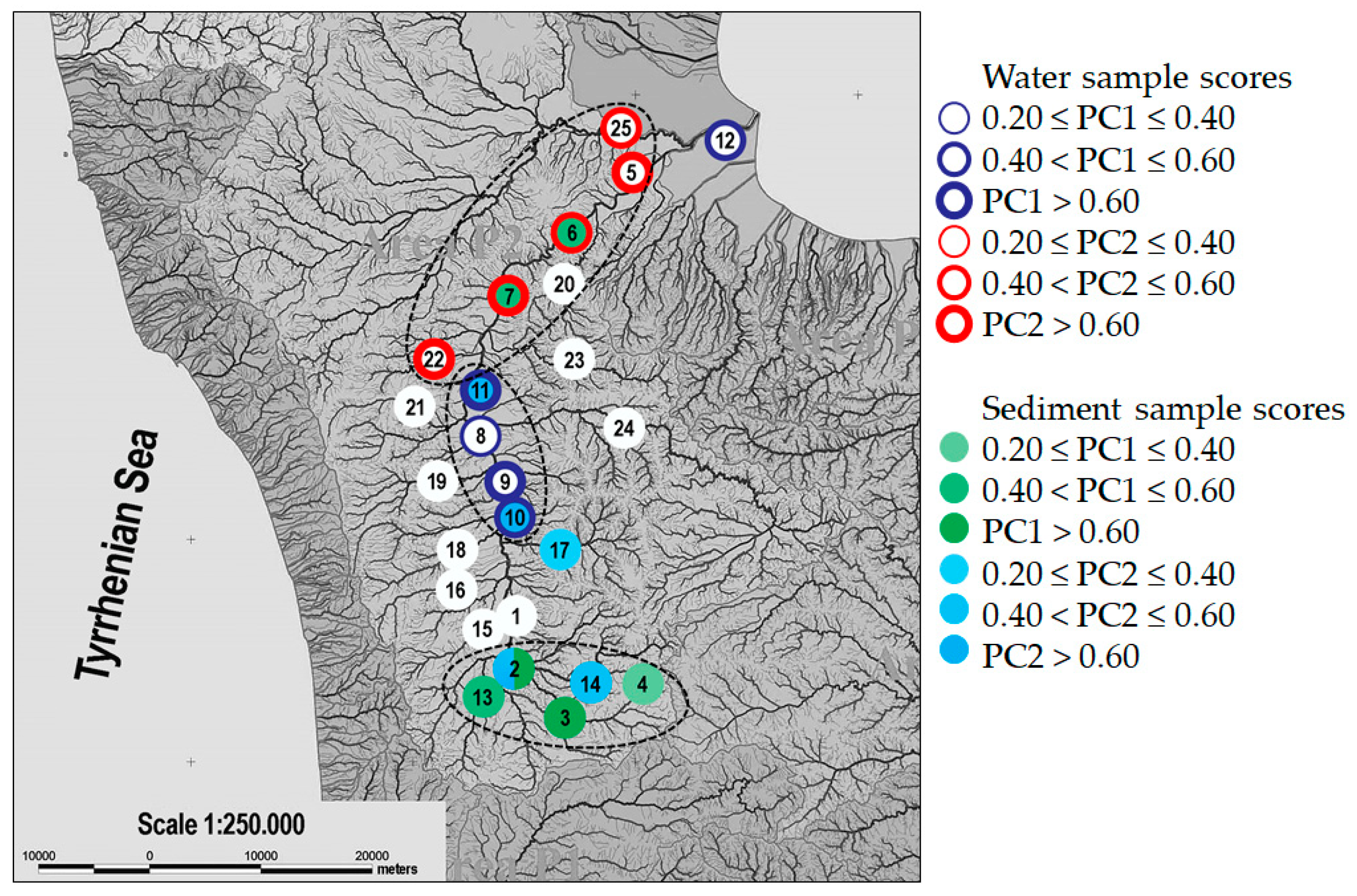
According to the results represented in both bi-plots, a risk map can be elaborated, as reported in Figure 5.

The water and sediment withdrawal sites were colored according to the values of the PC1 and PC2 scores [31]. PC1 in water monitoring (29.0% of explained variance, EV) showed higher positive loading values for nitrogen, P and As content, by identifying a corresponding cluster of samples in the risk map. Samples near the river source and the main tributary channel have similar characteristics regarding ammonium, total nitrogen, chromium and nickel, which remain at relatively lower values than in the other sampling points. For the withdrawals along the Crati Valley, Crati 4, 7, 8, 9 and 10, similar values are obtained for the arsenic, total nitrogen, ammonia, phosphorus and nickel parameters, with values above average (Figure 5). Information stored in PC2 (19% EV) grouped the samples collected at the mouth of the river, Crati 1, 2, 3, Coscile and Turbolo, have similar concentrations of total chromium, selenium and boron. It should be noted that, in this territorial area, the tributaries have similar characteristics to the sites near the river mouth, probably due to the fact that the effluent withdrawals were also made downstream and therefore can be enriched or contaminated by the same pollutants. This type of pollution could be due to anthropogenic activities in the sampling sites studied. In fact, in this area, it was possible to detect the presence of construction sites, agricultural crops and landfills.

The analysis of sediment showed less correlation between the samples and geographic location. However, through PCA and the graphical reports (bi-plots), it was possible to outline a distribution of the withdrawal points on the risk map. In particular, PC1 (49% EV) contained information relating to cadmium, zinc, copper, iron, aluminum, nickel and chromium, with a cluster of samples characterized by high concentrations of these parameters in Crati 2, 3, 15, 16, 17 and Busento. PC2 (17% EV) described the cluster of the samples Arente, Cardone, Crati 8, 9 and 15 as having higher values of mercury, arsenic and lead. The Crati 8 and Cardone sites had high values of mercury and Crati 9 a concentration of lead above the allowed limits. The analyzed data showed that the limits established by the environmental quality standards reported in the Decree 260 of 08/11/2010 were exceeded only with regard to the analysis of metals.

Many metals are dangerous because they insidiously penetrate our bodies through various vectors and tend to accumulate. Polluted surface waters can be included among the main culprits of these types of contaminants. In general, the values that exceed the limits established by current legislation are due to the anthropic activities that gravitate to the sampling sites: construction sites, agricultural crops and, in particular, the presence of industrial waste landfills, without excluding the biological crops.

As highlighted in the present work, multivariate analysis can be very useful in the production of a risk map that highlights the most critical areas and provides indications to the territorial control offices.

5. Conclusions

The monitoring of the Crati River in southern Italy was carried out for a period of 7 months by analyzing the waters and sediments of 25 sampling sites distributed along the river and its main tributaries. Two data sets were built, each including 750 values, recording 30 analytical parameters per site and processed with multivariate methods. These procedures first allowed the selection of the parameters carrying the most useful information. The selected data were elaborated by principal component analysis with the aim to find the relationship between the chemical composition of the sampling sites and the different geographical locations. The multivariate analysis allowed the clustering of the samples and the elaboration of a risk map. The results showed that, in the sites close to the river source, there was a concentration above the allowed limits of chromium in the water and nickel in the sediments, probably due to the presence of construction material. In the Crati Valley, however, where most of the inhabited centers are concentrated and therefore the presence of waste and landfills is massive, there are high levels of mercury, nickel and lead, both in water and in sediments. The sites near the river mouth had concentrations higher than the norm of chromium and nickel, in both matrices analyzed. The chemometric models have proven to be valid for the characterization of the environmental matrices. They are a useful tool to objectively and reliably describe the quality level of water and sediment matrices and to highlight the changes that can prove dangerous for the local population. The predictive capabilities of the model provide a valid means for routine analysis, at the service of the offices that manage and control water and intervention strategies. In fact, the obtained results allowed us to produce a risk map able to provide information to better assess the risk of pollution and provide assistance to communities to help them act to reduce risks to human health and the environment.

References

- Bandow, N.; Gartiser, S.; Ilvonen, O.; Schoknecht, U. Evaluation of the impact of construction products on the environment by leaching of possibly hazardous substances. Environ. Sci. Eur. 2018, 30, 14. [Google Scholar] [CrossRef] [PubMed]
- Skrbic, B.D.; Kadokami, K.; Antic, I. Survey on the micro-pollutants presence in surface water system of northern Serbia and environmental and health risk assessment. Environ. Res. 2018, 166, 130–140. [Google Scholar] [CrossRef] [PubMed]
- Grace, M.A.; Clifford, E.; Healy, M.G. The potential for the use of waste products from a variety of sectors in water treatment processes. J. Clean. Prod. 2016, 137, 788–802. [Google Scholar] [CrossRef]
- Kong, L.; Kadokami, K.; Wang, S.; Duong, H.T.; Chau, H.T.C. Monitoring of 1300 organic micro-pollutants in surface waters from Tianjin, North China. Chemosphere 2015, 122, 125–130. [Google Scholar] [CrossRef] [PubMed]
- Ahmad, I.; Chelliapan, S.; Othman, N.; Mohammad, R.; Kamaruddin, S.A. A review of municipal solid waste (MSW) landfill management and treatment of leachate. Int. J. Civ. Eng. Technol. 2018, 9, 336–348. [Google Scholar]
- De Luca, M.; Oliverio, F.; Ioele, G.; Husson, G.P.; Ragno, G. Monitoring of water quality in South Paris district by clustering and SIMCA classification. Int. J. Environ. Anal. Chem. 2008, 88, 1087–1105. [Google Scholar] [CrossRef]
- Box, G.E.P.; Draper, N.R. Empirical Model-Building and Response Surfaces; John and Wiley and Sons: New York, NY, USA, 1987. [Google Scholar]
- Draper, N.; Smith, H. Applied Regression Analysis; John and Wiley and Sons: New York, NY, USA, 1981. [Google Scholar]
- Jackson, J.E. A User’s Guide to Principal Components; John and Wiley and Sons: New York, NY, USA, 1991. [Google Scholar]
- Krzanowski, W.J. Principles of Multivariate Analysis. A User’s Perspective; Oxford Press: Oxford, UK, 1998. [Google Scholar]
- Mardia, K.V.; Kent, J.T.; Bibby, J.M. Multivariate Analysis; Academic Press: London, UK, 1998. [Google Scholar]
- Muangthong, S.; Shrestha, S. Assessment of surface water quality using multivariate statistical techniques: Case study of the nampong river and songkhram river, Thailand. Environ. Monit. Assess. 2015, 187, 548. [Google Scholar] [CrossRef] [PubMed]
- Ragno, G.; Ioele, G.; De Luca, M.; Garofalo, A.; Grande, F.; Risoli, A. A critical study on the application of the zero-crossing derivative spectrophotometry to the photodegradation monitoring of lacidipine. J. Pharm. Biomed. Anal. 2006, 42, 39–45. [Google Scholar] [CrossRef] [PubMed]
- Ragno, G.; Vetuschi, C.; Risoli, A.; Ioele, G. Application of a classical least-squares regression method to the assay of 1, 4-dihydropyridine antihypertensives and their photoproducts. Talanta 2003, 59, 375–382. [Google Scholar] [CrossRef]
- Zhang, X.; Wang, Q.; Liu, Y.; Wu, J.; Yu, M. Application of multivariate statistical techniques in the assessment of water quality in the Southwest New Territories and Kowloon, Hong Kong. Environ. Monit. Assess. 2011, 173, 17–27. [Google Scholar] [CrossRef] [PubMed]
- Zhou, F.; Liu, Y.; Guo, H. Application of multivariate statistical methods to water quality assessment of the watercourses in Northwestern New Territories, Hong Kong. Environ. Monit. Assess. 2007, 132, 1–13. [Google Scholar] [CrossRef] [PubMed]
- De Luca, M.; Ragno, G.; Ioele, G.; Tauler, R. Multivariate curve resolution of incomplete fused multiset data from chromatographic and spectrophotometric analyses for drug photostability studies. Anal. Chim. Acta 2014, 837, 31–37. [Google Scholar] [CrossRef] [PubMed]
- Dinc, E.; Ragno, G.; Ioele, G.; Baleanu, D. Fractional wavelet analysis for the simultaneous quantitative analysis of lacidipine and its photodegradation product by continuous wavelet transform and multilinear regression calibration. J. AOAC Int. 2006, 89, 1538–1546. [Google Scholar] [PubMed]
- Rizeei, H.M.; Azeez, O.S.; Pradhan, B.; Khamees, H.H. Assessment of groundwater nitrate contamination hazard in a semi-arid region by using integrated parametric IPNOA and data-driven logistic regression models. Environ. Monit. Assess. 2018, 190, 633. [Google Scholar] [CrossRef]
- Gumma, M.K.; Pavelic, P. Mapping of groundwater potential zones across Ghana using remote sensing, geographic information systems, and spatial modeling. Environ. Monit. Assess. 2013, 185, 3561–3579. [Google Scholar] [CrossRef]
- Idrografico, M.d.L.P.-S. Le Sorgenti Italiane: Elenco E Descrizione, Pubblicazione N. 14 Del Servizio, Vol. VI, Calabria (Con Bacini Lucani Con Foce Al Tirreno); Istituto Poligrafico dello Stato: Roma, Italy, 1941. [Google Scholar]
- Dlsg N. 60. Quadro Per L’azione Comunitaria in Materia Di Acque; Direttiva del Parlamento Europeo e del Consiglio, ISPRA: Roma, Italy, 2000. [Google Scholar]
- APAT-IRSA. Metodi Analitici Per Le Acque; I.G.E.R. srl: Capannori, Italy, 2003; Volume 1. [Google Scholar]
- APAT. Protocollo Per Il Campionamento Dei Parametri Fisico-Chimici a Sostegno Degli Elementi Biologici Nei Corsi D’acqua Superficiali; APAT: Rome, Italy, 2007. [Google Scholar]
- Balzamo, S.; Carere, M.; Ferrara, F.; Macchio, S.; Polesello, S.; Rusconi, M. Le sostanze prioritarie nel biota: Criteri per il monitoraggio e i metodi di analisi. Biol. Ambient. 2017, 31, 1–6. [Google Scholar]
- Dlsg N. 152. Norme in Materia Ambientale; ISPRA: Roma, Italy, 2006. [Google Scholar]
- Dlsg N. 230. Radiazioni Ionizzanti E Radioprotezione; ISPRA: Roma, Italy, 1995. [Google Scholar]
- Dlsg N. 260. Criteri Tecnici Per La Classificazione Dello Stato Dei Corpi Idrici Superficiali. Modifica Norme Tecniche Dlgs 152/2006; ISPRA: Roma, Italy, 2010. [Google Scholar]
- ISPRA. Linee Guida Per Il Monitoraggio Della Radioattività; Consiglio Federale delle Agenzie Ambientali: Roma, Italy, 2012.
- UNI 9882. Determinazione Dei Principali Radionuclidi Nel Latte; Ente Italiano di Normazione: Milano, Italy, 1991.
- Tepanosyan, G.; Sahakyan, L.; Belyaeva, O.; Saghatelyan, A. Origin identification and potential ecological risk assessment of potentially toxic inorganic elements in the topsoil of the city of Yerevan. J. Geochem. Exp. 2016, 167, 1–11. [Google Scholar] [CrossRef]
© 2020 by the authors. Licensee MDPI, Basel, Switzerland. This article is an open access article distributed under the terms and conditions of the Creative Commons Attribution (CC BY) license (http://creativecommons.org/licenses/by/4.0/).