1. Introduction
From different studies and witnessed abnormalities around the globe, it is now clear that climate change has brought and will bring vulnerabilities. CO
2 in the atmosphere has set the record in 2018 since preindustrial era (1850–1900) [
1]. Consequently, global mean temperature has been rising 1.5 °C above preindustrial (1850–1900) era [
1]. Other key indicators of the critical situation are Sea Level Rise (SLR) and Sea Ice Extent (SIC); both are the direct consequence of greenhouse gas (GHG) increase in the atmosphere. SLR has hit the record in 2019 of 3.2 mm/year during the 1993–2019 period and also Arctic extent has been decreasing [
1]. On the local scale, the warming has been consistent with the weather and climate variabilities related to climate change; North America has been unusually cold due to the crisis [
1]. Extreme precipitations, more frequent hurricanes, intense tropical cyclones, unexpected thunderstorms and tornados, severe cold breaks, prolonged droughts, and seasonal timing shifts are expected to be common ([
2,
3,
4,
5,
6,
7]). These threats not only target human communities but also do threaten ecosystems functionality.
Significant changes in hydrological regimes in most part of the land surface of the planet will be likely to occur by midcentury (2050) [
8]. The Fourth Assessment Report (AR4) [
9] of the Intergovernmental Panel for Climate Change (IPCC) regarding the anthropogenic impact on the hydrological cycle like precipitation, snowmelt, and earlier spring peak flows, reported medium to high confidence where the latter was very likely ([
9,
10]). Climate change will adversely change streamflow and water quality and consequently will jeopardize freshwater ecosystems [
11].
In Southeast of the US, seasonal drying has been observed for spring, fall, and winter and in summer the soil moisture increased during 1988–2010 [
10]. Although potential evapotranspiration (PET) is projected to increase, evapotranspiration (ET) as the 2nd largest component of the hydrological cycle requires further studies to see possible implications ([
10,
12]). Projections show 4.3 °C and 7.72 °C rise by mid-century (2036–2065) and late-century (2071–2100) under RCP 8.5, respectively [
13]. Projections under RCP 8.5 by mid-century also reveal 40–50 days per year with temperature greater than 32 °C as a key temperature threshold [
13]. Changes in numbers of nights below 0 °C show an increase of 10–15 days for the Southeast [
14]. Projected warm weather will increase ET, leading to reduced water availability and ground water recharge ([
15,
16,
17]). Uptake of soil water by forests is expected to increase, leading to decline in water yield under increased temperature and decreased precipitation in the Southeast region including Alabama ([
15,
16]). Longer growing season and increased wildfire likelihood were also projected for southeast US forests [
18]. Projected population growth and land use change will worsen the situation and pose a threat to the economy and unique ecosystems, and land use change in the Southeast, which ultimately exacerbates water scarcity, is faster than in any other areas in the US [
19].
The Southeast has been categorized as the second most vulnerable region to weather and climate disasters in the US for the past three decades (1980–2012). Hurricanes can be considered as disasters for the coastal area, and tornados and storms are disasters for inland regions where they are close to the gulf and Atlantic coasts [
19]. Many factors contribute to the climate of the Southeast region including closeness to the Atlantic Ocean and the Gulf of Mexico and El Nino-Southern Oscillation (ENSO), and land falling tropical weather systems [
14]. Projections for annual runoff and consequent stream flow in the Southeast indicate declines, which is consistent with long-term (multi-seasonal) droughts [
10]. Moreover, historically, river floods have been decreasing in most parts of the Southeast at least 6% percent per decade ([
10,
20]). River floods are more complex as a direct result of the heavy precipitation, and topography, soil moisture, channel condition, and anthropogenic influences such as land use change are thought to play the key roles [
10]. These highlight the importance of hydrological analysis with respect to non-stationary stressors in the region.
Few studies like Ge Sun et al. [
16] have studied the impact of climate change in watershed scale in the Southeast. They demonstrated the importance of water supply stress and showed increase in runoff and sediment yield due to increase in erosivity and/or vegetation cover loss. They also stated that climate change and possible future stressors like population growth, land use change (LUC), energy security, and policy shift would interact with surface and groundwater availability [
16].
There are LUC impact studies, but the land use scenarios are limited. Chen et al. [
21] investigated only agricultural land use change and projected 12% to 20 % decline in crop ET by the mid and end of the 21st century, respectively [
21]. Qihui Chen et al. [
22] have studied the effect of historical LUC within a watershed in China and found small impacts on hydrological extremes [
22]. Villamizar et al. [
23] have studied LUC within a watershed in Colombia with 3 hypothetic LUC and identified strategic points for conservation practices [
23]. Marhaento et al. [
24] studied climate and LUC in a tropical watershed in Indonesia and found intensification in annual stream flow and surface runoff if the drivers combined; the LUC scenarios used in the study were based on extrapolation of trends [
24]. Separate and combined effect of climate and LUC were investigated by Tamm et al. [
25], and they found strong linear correlation forest cover change and annual runoff. Their study area was heavily forested, and afforestation and deforestation LUC scenarios were used [
25]. Wang et al. [
26] have studied a coastal watershed in southwest Alabama using a spatially explicit LUC based on population growth. They found small effects in changes in streamflow but significant changes in partitioning streamflow causing higher surface runoff [
26]. Impacts of afforestation and deforestation on hydrological response have also been studied ([
18,
27,
28]); and consistent results have not been an outcome of the impact of forest on water yield [
27]. There are few LUC impact studies in the Southeast of the US; and the Southeast region in the US has been experiencing rapid LUC comparing to other regions in the country [
29]; therefore, there is a need for LUC impact studies in this region.
Moreover, catchment specific characteristics like seasonality and storm frequencies have implications in the flood peaks [
30]. Natural hazards like drought, flood, and in general vulnerabilities produced by climate are results of regional behavior not global ([
31,
32]). Moreover, it is essential to improve regional projections to determine the mechanisms of the regional forcings and related climate impacts clearly [
33]. Although, most studies on hydrological future projections have come to the conclusion that water balance components will be affected under climate scenarios, the hydrological response itself varies depending on region-specific characteristics, topography, geography, location, and precipitation regimes [
28]. Previous studies have revealed the general impacts of climate change for the entire Southeast of the US. On the other hand, since climate variables should be calculated to investigate climate change impact on hydrology, it is necessary to couple an improved downscaled General Climate Models (GCMs) with SWAT [
34]. In the past few years, researchers have used the predecessors of the GCMs ([
28,
31,
34,
35]). Therefore, in this study we coupled an improved downscaled GCMs on the watershed scale, in the Southeast of the US.
The novelty of the work is that we used the Coupled Model Intercomparison Projects–Phase 5 (CMIP5) downscaled data with increased robustness and detailed outcome combined with new LUC projections based on the Shared Socioeconomic Pathways (SSP). These maps are consistent with four IPCC emissions scenarios with improved demographic and spatial allocation models. We carried out the investigation on the subbasin scale with new developed techniques for data preparation. This study provides greater details on combined effects of the drivers for a better understanding of the hydrological processes in the Southeast of the US. The findings provide the basis to analyze combinations of what conservation practices and when and where may have the least impact on natural land cover, while incorporating socioeconomic planning. This study better integrates direct relation and feedbacks between future land use pattern and their influence on land cover and resulting changes in hydrological response (water balance variables). Mitigation activities and adaptation planning across related sectors can benefit from stablishing this type of data and the findings. The results can be put into the overall research body and also can serve as a basis for comparison and decision-making processes.
We used SWAT for hydrological modeling and coupled it with three representative GCM models in which the data are downscaled using a new developed method called Localized Constructed Analogs (LOCA). The goals of the study are (i) to establish a robust hydrological model for the watershed, (ii) to couple the detailed projections with a new downscaling method as well as new LUC scenarios, and (iii) to analyze the response of the watershed to the future stressors.
4. Future Climate Data
A set of benchmark emissions scenarios referred to Representative Concentration Pathways or RCPs [
57] are possible development trajectories for the main climate change drivers [
58]. Research on the multi-gas emissions scenarios were the base of the RCPs development ([
59,
60,
61,
62,
63,
64]). They collectively encompass (extending to year 2100) radiative forcing values from 2.6 to 8.5 W/m
2 relative to year 1750 (59, 27). These scenarios are as follows: RCP2.6, RCP4.5, RCP6, and RCP8.5. RCP 2.6 is a mitigation scenario, and its goal is to keep the global mean temperature rise under 2 °C ([
57,
65,
66]). The radiative forcing for RCP2.6 increases up to around 3 Watts per square meter (W/m
2) before 2100 and then declines ([
66,
67]). Under RCP4.5 and RCP6, concentration of GHGs are stabilized (without overshoot) after 2100 [
65]. RCP4.5 stops increasing radiative forcing at 4.5 W/m
2 by year 2100, and the forcing becomes constant afterward [
68]. RCP6 pathway controls the increasing radiative forcing at 6 W/m
2 without exceeding the value afterward [
69]. GHGs emissions increase by around 2060 and then decline until 2100 [
69]. RCP8.5 assumes high population and slow economic growth, which leads to increasing GHGs emissions resulting in radiative forcing as high as 8.5 W/m
2 by the end the 21st century, and it is assumed to rise afterward [
70]. Additional actions are required to halt continuously rising level of GHG concentrations, which are due to the growth of global population and economic activities [
71]. These actions are dependent on the political and socio-economic conditions on the global scale ([
63,
66]). Taking the current global political condition and its possible future pathway into account, we selected the RCP 4.5 and RCP6.0 as moderate and severe pathways, respectively.
The General Climate Models (GCMs) use these RCPs to produce future climate data. The main source of climate projections is the modeling results of the Coupled Model Intercomparison Projects (CMIP3 and CMIP5) [
28]. Since GCMs’ horizontal resolution is low, it is difficult to derive regional scale climate information from them [
72]. In general, GCM results are not reliable for models with resolution less than 200 km [
73]. Hydrological processes occur on a scale (in order of 10 km) at which GCMs (resolution of 1° to 2.5° latitude-longitude) cannot provide reliable results ([
74,
75]). Moreover, GCMs are not able to capture frequency and magnitude of extreme events ([
76,
77]). Therefore, for important climate variables like precipitation and temperature, it is necessary to use higher resolution. Downscaling techniques have been used rigorously to produce climate variables from GCMs on the desired scale for hydrological modeling of climate change impact studies ([
28,
78,
79]). Between two types of the existing downscaling techniques which are dynamical and statistical, we used the statistical downscaling method. Statistical method downscales GCMs’ output based on the historical relationship between large- and small-scale conditions [
80]. In this study, we used a statistical downscaling called Localized Constructed Analogs (LOCA). LOCA chooses analog days from observed data and applies a multiscale spatial matching scheme to estimate suitable downscaled climate variables [
80]. More realistic regional patterns of precipitation, better estimates of extreme events, and reduced number of light-precipitation days are the advantages of LOCA [
80]. More information on LOCA can be found here:
http://loca.ucsd.edu/ [
81].
Considering the complexity of the GCMs, CMIP5 outputs are inevitably biased ([
82,
83]). Bias correction (BC) is the process of transforming GCM outputs using algorithms in order to adjust the outputs ([
35,
83]). Basically, biases are detected by comparing the observation and simulation results, and then, they are used to correct baseline and projections ([
35,
83]). Bias-corrected inputs for hydrological modeling improve the result; hence, bias correction is needed for GCMs output ([
84,
85]). LOCA as a downscaling technique was improved by constructed analogs (CA) process containing a bias correction step ([
80,
86]). The BC in LOCA includes 3 steps. First, a preconditioning technique is used to correct the annual cycle, and then, two different distribution techniques are used, one for temperature and one for precipitation, and finally, a frequency-dependent bias correction (FDBC) is used to adjust the sequencing of variation for different time scales, since the sequencing for GCM outputs potentially differs from observed ones ([
84,
87]). We obtained and analyzed CMIP5 output, the LOCA dataset, for three models, CCSM4, GISS-E2-R, and GFDL-CM3, under RCP4.5 and RCP6.0 from Downscaled CMIP5 Climate and Hydrology Projections (
https://gdo-dcp.ucllnl.org/) ([
82,
88,
89,
90,
91]). The downloaded data are bias-corrected 1/16th degree latitude-longitude (~6 km × 6 km) daily precipitation (mm/day), and maximum and minimum temperature (°C) projections. Hereafter, the downloaded dataset, which is downscaled and bias corrected by LOCA, is referred to as “the CMIP5 multi-model ensemble LOCA”. The LOCA dataset contains future projections under RCP4.5 and RCP6.0 for 32 GCMs for the conterminous US from 1950 to 2099. For selected models, errors w.r.t. of observation from Livneh et al. [
92] in the Southeast of the US are less than 5%, 0.5 °C, and 0.5 °C for daily precipitation, daily maximum temperature, and daily minimum temperature, respectively ([
80,
92]). From the evaluation and verification results, it can be concluded that the LOCA performance is better for the Southeast region compared to other regions across the US (
http://loca.ucsd.edu/).
In hydrological projection process using GCMs, their initial condition, future scenarios, and hydrological model incorporate uncertainties to the result [
93]. Ouyang et al. [
94] have concluded that different results in the future projections are partially due to the different climate models [
94]. Considering the many numbers of the GCMs and the variability they could cover based on the model skill and independency, we selected the three models to be able to analyze broad extents of changing climate variables within the UCS; in this way, we were able to address the uncertainty ([
28,
95,
96]). Locating and Selecting Scenarios Online (LASSO) tool from Environmental Protection Agency (EPA) (
https://lasso.epa.gov/) was used to filter out the selected model from 32 GCMs. Through the different steps of the tool, we have examined climate parameters variabilities with two time periods (annual and seasonal) and selection strategies to reach the goal of three representative models. Models’ name, their associated institution, type of experiment, and ensemble member are shown in
Table 3 [
97].
5. Scenario Development
Two projection periods, both under RCP4.5 (moderate) and RCP6.0 (severe) were presented, mid-century (2040–2069) and late-century (2070–2099). The results of hydrological simulation were shown in monthly, seasonal, and annual time scales. The seasons were defined as DJF (winter: December, January, February), JJA (summer: June, July, August), MAM (spring: March, April, May), and SON (fall: September, October, November).
SWAT incorporates CO
2 to account for its impact on plant water requirements and on level of the potential evapotranspiration (PET) [
46]. It takes the CO
2 concentration amount as a single input value for each subbasin. The CO
2 concentration values for the historical and future projections are shown in
Table 4. The values are derived from [
67].
Projected population for the conterminous US indicates significant increase in demand for food, energy, and urban development [
98]. From 2001 to 2011, the Southeast region (AL, AR, FL, GA, KY, LA, MS, NC, SC, TN, and VA) has lost more than 100 and 1400 sq
2 agricultural land and forest, respectively, and gained 600 sq
2 developed land cover [
99]. For UCS and Pea and Yellow River Subbasin, farming land decreased 27.21% and urban area increased 42.55% from 1992 to 2011 [
38]. Regarding land use condition in the future, there have been few studies (national US and global scale) based on different scenarios including Special Report on Emissions Scenarios (SRES), RCP, and Shared Socioeconomic Pathways (SSP) by the Intergovernmental Panel for Climate Change (IPCC) ([
98,
99,
100,
101,
102,
103]). Sohl et al. [
98] using a different land use forecasting model has predicted 22.9% to 61% increase in urban land cover for conterminous US by the year 2050. They projected noticeable loss of natural covers, which was due to expansion of anthropogenic land uses. The fourth National Climate Assessment reported 50% and 80% increase in urban land use allocation by 2100 under SSP2 and SSP5, respectively, with 2010 land use condition as the baseline [
99]. To account for these changes, we obtained and analyzed projected land covers for each decade until 2100 from the Fourth National Climate Assessment dataset through Global Change Explorer (GCX) [
104]. The land use scenarios (land-use change scenarios for the conterminous United States forecast decadally from 2000 to 2100) used in this study are the results of the Integrated Climate Land Use Scenario ICLUSv.2 model. ICLUS couples demographic growth model with a spatial allocation model (Spatially-Explicit Regional Growth Model (SERGoM) [
105] and produces land use scenarios consistent with IPCC [
102]. Bierwagen et al. [
106] has studied the model and related components. The maps were verified by developing a regression tree model and with values from three “ground-truth” datasets generated from high-resolution aerial photography, which showed good fit of R
2 = 0.96 (y = 0.624x + 5.730). They also compared conditions in 1989 for 56 watersheds (14-digit Hydrologic Unit Code) and found good fit with R
2 = 0.96y = 0.823x − 1.060) [
106]. These maps are based on SSP scenarios with 19 land cover classes ([
106,
107]). One possible caveat, however, is that there is not much agreement between different forecasting models, and they appear to be at the initial stage of development [
102]. Future projection results for all models in this study were presented in monthly, seasonal, and annual averages and compared to the historical result to analyze the future hydrological condition within the UCS. Then, we did the same comparison for SWAT simulation, mainly discharge. Corresponding land use projections to projection periods (mid-century and end-century) were used in SWAT modeling to simulate the discharge and evapotranspiration (ET). Finally, we used box plots to show the changes of the climate and hydrological variables.
SWAT: For this study we used Soil and Water Assessment Tool (SWAT). SWAT is assemblages of mathematical equations representing different parts of the hydrological cycle including movement, fate, and transport of water and sediments and nutrients in and on soil, through groundwater, and in river streams and reservoirs ([
108,
109]). The development of the model started in the early 1990s, and it has been evolving by USDA (United States Department of Agriculture) agricultural Research Service (ARS) ([
110,
111]). It is a process-based and semi-distributed continuous-time river basin scale model ([
110,
112]). It has been written in Fortran language including more than 310 subroutines representing different parts of the hydrological and bio-geochemical processes ([
112,
113]). It was originally developed to evaluate water resources management and Nonpoint Source (NPS) pollution in large river basin [
110]. It has proven to be effective for its purposes and computationally efficient and can be used for long term continuous simulation including climate change impact studies ([
110,
111]). It operates on a daily time step and outputs daily, monthly, and yearly results ([
110,
111]). SWAT splits a watershed into subwatersheds that are further split into hydrologic response units (HRUs) ([
110,
111]). HRUs are nonspatial units and unique combination of homogeneous land use, soil, slope, and management characteristics ([
110,
111]). This gives SWAT the capability to model surface runoff, infiltration, soil water movement, ET, in-stream transformations, sediment movement, canopy interception, plant uptake, and nutrients circulation including biogeochemical processes at HRU level [
46]. Main components of a SWAT model for a given watershed are weather, hydrology, erosion/sedimentation, plant growth, nutrients, pesticides, agricultural management, stream routing and pond/reservoir routing [
113]. Simulation in SWAT has two parts, land phase and routing phase; in land phase, the amount of water, sediment, nutrient, and pesticide loadings are regulated into the main channel in each subbasin, and in the routing phase, in- stream processes including water movement, sediment transport, and the nutrients loading are simulated ([
46,
110]). In SWAT, water balance is the base of all the processes, and the hydrological cycle is climate driven; thus, SWAT requires precipitation, minimum and maximum temperature, solar radiation, relative humidity, and wind speed in daily time scale ([
110,
114]).
SWAT uses Equation (1) to simulate water balance ([
46,
108]):
where
and
are soil water content for beginning and end of the model, respectively.
t (day) is time.
is rainfall;
is surface runoff;
is evapotranspiration;
is percolation to vadose zone, and
is return flow amount, and all variables are in mm ([
46,
108]).
Water yield as part of subbasins blue water is the amount of water after leaving HRUs and entering the main channel is calculated with Equation (2) ([
46,
47,
115]):
where WYLD is the amount of water yield,
is surface runoff,
is return flow amount,
is the amount of lateral flow,
is transmission losses, and the abstracted water from the pond; all variables are in mm ([
34,
47,
116]).
In SWAT, surface runoff can be estimated in two ways: SCS (Soil Conservation Service) runoff curve number method (USDA-SCS, 1972) and the Green and Ampt infiltration method (1911) [
46]. We used the former. Equation (3) is SCS runoff curve number method ([
46,
108]):
where
is surface runoff;
is rainfall; and
S is retention parameter. 0.2
S is estimated as the initial abstraction including surface storage [
46]. Retention parameter varies through the watershed and time owing to changes in soil, land use, and management [
46].
S is estimated as follows:
where
CN is the curve number which is adjusted for different soil moisture level and slope [
46].
For surface runoff Equation (3) was used. For flow routing the variable storage coefficient method were used ([
46,
117]). Since our modeling required simulation of CO
2 climate change effects, the Penman–Monteith method was used for calculation of potential evapotranspiration ([
118,
119,
120]). Actual Evapotranspiration (AET) was calculated by procedure established by Richtie [
121]. The UCS was delineated into 54 subbasin and 1821 HRUs. “SWAT2012 rev64” version was used to perform the modeling.
6. Calibration
Calibration can be manually done or through a combination of manual and auto calibration procedures [
122]. Our approach to calibrate and validate was the later through a split-sample strategy [
122]. To evaluate the performance of the model, we have first carried out a sensitivity analysis (SA) manually and then using SWAT Calibration and Uncertainty Procedures (SWAT-CUP) to filter out insensitive parameters to reduce the computational workload of the calibration ([
123,
124,
125,
126]). Sensitivity analysis is to estimate how much model outputs change with respect to each model parameter (input) change ([
110,
126]). First, a set of parameters were selected according to UCS hydrologic characteristics and the literature ([
110,
127,
128,
129,
130,
131,
132]). Then, using one-factor-at-a time sensitivity analysis, initial parametrization was carried out and parameters were optimized, and their initial ranges were predicted ([
127,
133,
134]). After a set of manual calibration using the first set of parameters, we used SWAT-CUP to modify the selected parameters and perform sensitivity and uncertainty analysis [
110]. We used the Sequential Uncertainty Fitting version algorithm (SUFI2) within SWAT-CUP ([
132,
135]). The SUFI2 is based on the inverse modeling and is to estimate parameters using observed data ([
132,
135]). In other words, it uses initial large parameter uncertainty and through steps, decreases the uncertainty until the uncertainty range falls within a range/band called 95% Prediction Uncertainty (95PPU) ([
135,
136]). SUFI2 uses a global search approach to carry out optimization and uncertainty analysis, and it can handle many parameters ([
135,
136]). For accuracy quantification of the model, our objective function includes Nash–Sutcliffe Efficiency (NSE), Coefficient of Determination (R
2), Percent Bias (PBAIS), and RMSE-observations standard deviation ratio (RSR) ([
125,
137,
138,
139]). The metrics for satisfactory thresholds were selected based on the literature ([
127,
138,
140]).
Table 5 shows the objective function and the thresholds of the metrics and final results for calibration and validation periods. Following are the formulas used for these metrics.
where
is the ith measured stream flow;
is
ith simulated stream flow;
is the mean of observed stream flow data;
is the mean of simulated data, and
n the total number of observations.
NSE value between 0.0 and 1 is considered acceptable with 1 being the optimal value indicating the plot of observed versus simulated fits perfectly ([
138,
139]). For R
2, the higher the value, the lesser the error variance and values greater than 0.5 are considered to be acceptable ([
138,
140]). Negative PBIAS means overestimation, and positive PBIAS means underestimation, with 0 being the optimal value. RSR ranges from 0.0 to a positive large number, with 0.0 being the optimal condition meaning the RMSE is zero. The lower RSR, the lower residual variation, indicating better model performance [
138]. NSE, R
2, and RSR are unitless and PBAIS has the unit of the constituent being evaluated, which for our case is cms (m
3/s). The global sensitivity analysis (where all parameters are allowed to change through analysis) were carried out through SWAT_CUP to prioritize the most responsive parameters and remove parameters with smaller sensitivity from further sampling [
132]. Through the SA, a multiple regression analysis was used to determine the parameter sensitivity statistics (t-stat and
p-value) [
136]. t-stat and
p-value were used to describe the relative significance and significance of sensitivity, respectively [
116]. Sensitive parameters correspond to larger absolute t-stat values among the parameters and to smaller
p-values (close to 0; commonly accepted threshold is 0.05) [
136]. Based on the SA, the following parameters were identified as responsive: SOL_AWC (Available water capacity of the soil layer), RCHRG_DP (Deep aquifer percolation fraction), CH_K2 (Effective hydraulic conductivity in main channel alluvium), SLSUBBSN (Average Slope Length), ESCO (Soil evaporation compensation coefficient), GWQMN (Threshold water level in the shallow aquifer for the base flow), and ALPHA_BF (Baseflow alpha factor).
Table 6 shows final parameters and their fitted values. It is worth to mention that the SA result is the prediction of the average changes of the objective function being produced by changes in a given parameter as other parameters are also changing [
141]. p-factor and r-factor were also considered for SUFI2 performance evaluation as well as measuring the goodness of calibration ([
132,
135]). p-factor is the percentage of observations covered by the 95PPU, and r-factor is the ratio of the 95PPU average thickness and the standard deviation of the observations ([
127,
136]). The extent from 2.5% to 97.5% of the cumulative distribution of the simulated variable resulting from the Latin hypercube sampling is 95PPU ([
127,
132,
135]). p-factor ranges from 0 to 1; p-factor greater than 0.7 means acceptable goodness of fit; r-factor varies between 0 and infinity; here, r-factor less than 1.5 was considered satisfactory ([
127,
132,
135,
136]).
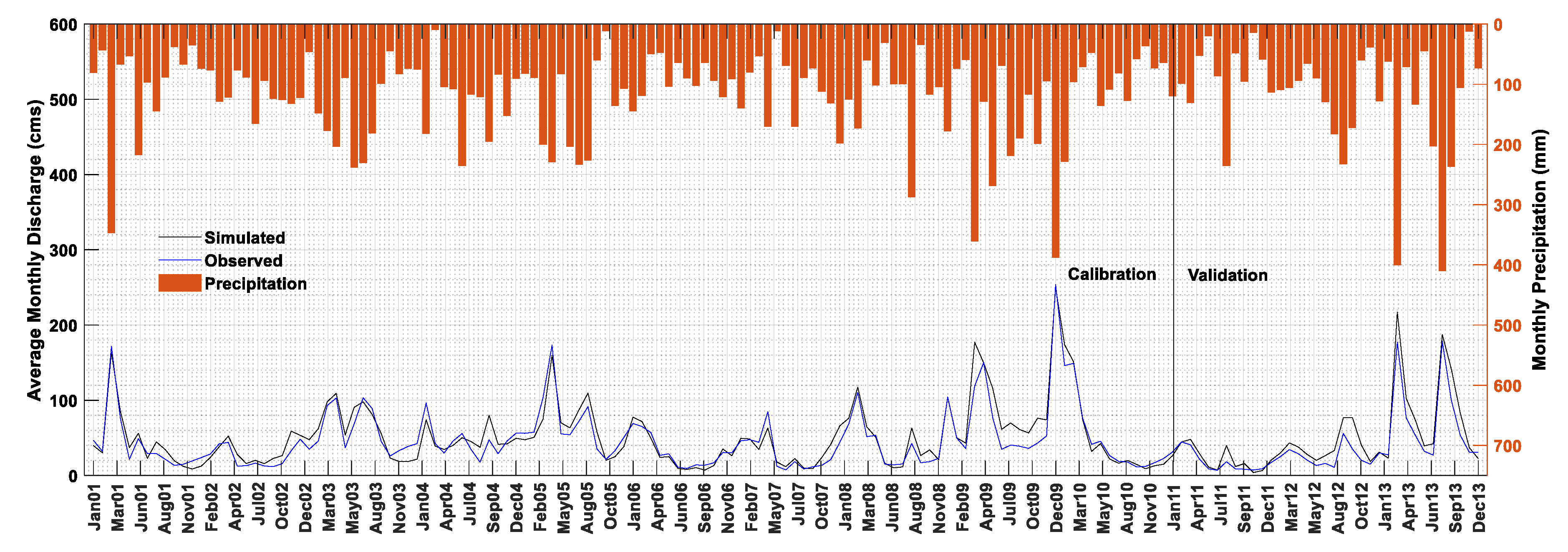
Table 5 shows the goodness of fit metrics. The selected parameters were used to calibrate SWAT at two USGS site (Newton (USGS2361000) and Bellwood (USGS2361500)) for subbasins 29 and 52, respectively. Observed data from the later site is used for SA and uncertainty analysis. The number of simulations was 450 with 4 iterations. SWAT was performed for the period from 1998 to 2013. The period from 1998 to 2000 was considered as warm up; the period from 2001 to 2010 was the calibration period and from 2010 to 2013 was the validation period. Given the final values for the model performance metrics (
Table 5) and the accepted thresholds, it was determined SWAT stream flow estimation for the UCS was efficient.
Figure 2 shows the calibration result for both calibration (2001–2010) and validation period (2011–2013).
7. Results and Discussion
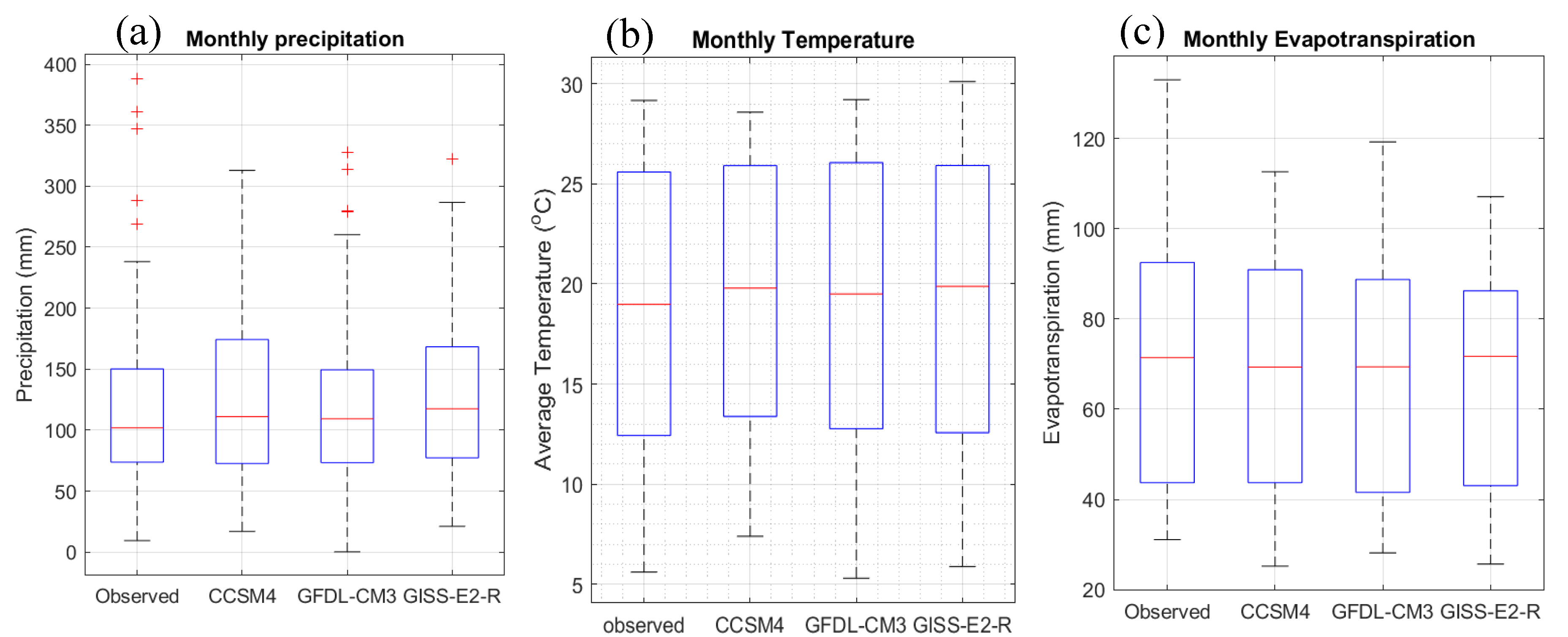
The CMIP5 multi-model ensemble LOCA results for precipitation and temperature during baseline period show consistency with the observed values (
Figure 3). Between the 3 models, GFDL-CM3 has the closest distribution to the observed precipitation with the 6.8% median difference and the closest number of outliers. The 25th percentile for the observation and GFDL-CM3 are 71.4 and 74.68 °C respectively. The 75th percentiles are the same (148.3 °C). Therefore, it indicates similar distribution.
Figure 3b illustrates the temperature distribution for the observed and baseline periods. It represents quiet similarity, especially for model GFDL-CM3, where the distance is between 25th and 75th percentile and the whiskers’ length are the same. The median difference of models (CCSM4, GFDL-CM3, GISS-E2-R) from the observed ones are 4.2%, 2.6%, and 4.7%, respectively. We also compared the baseline ET from the climate data with the observation period (
Figure 3c).
Figure 3c also demonstrates similar distribution from the 25th to the 75th percentiles from all datasets. However, upper whiskers for the observation is longer. This difference has no implication on the study, since here, we are not focused on extreme weather situations.
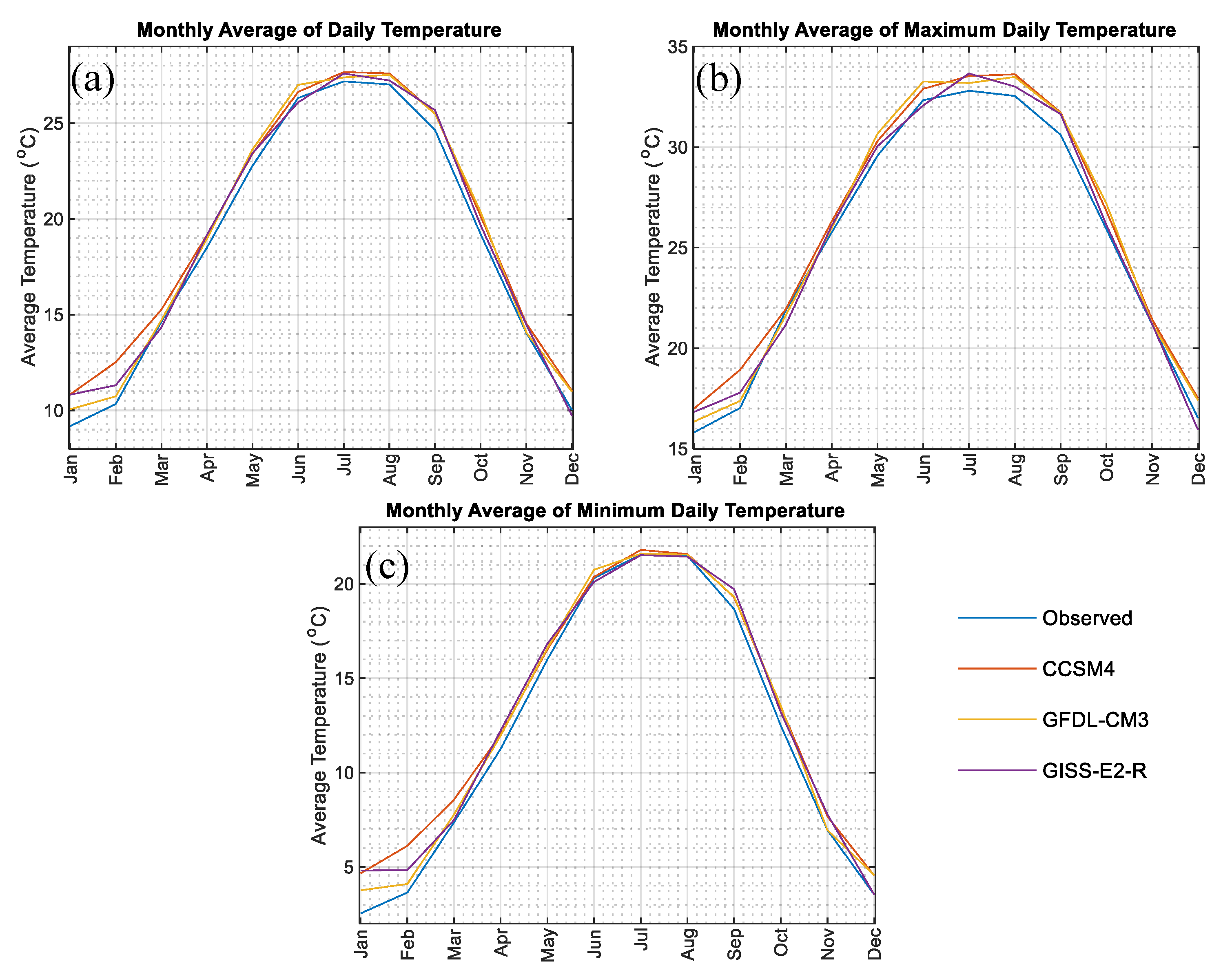
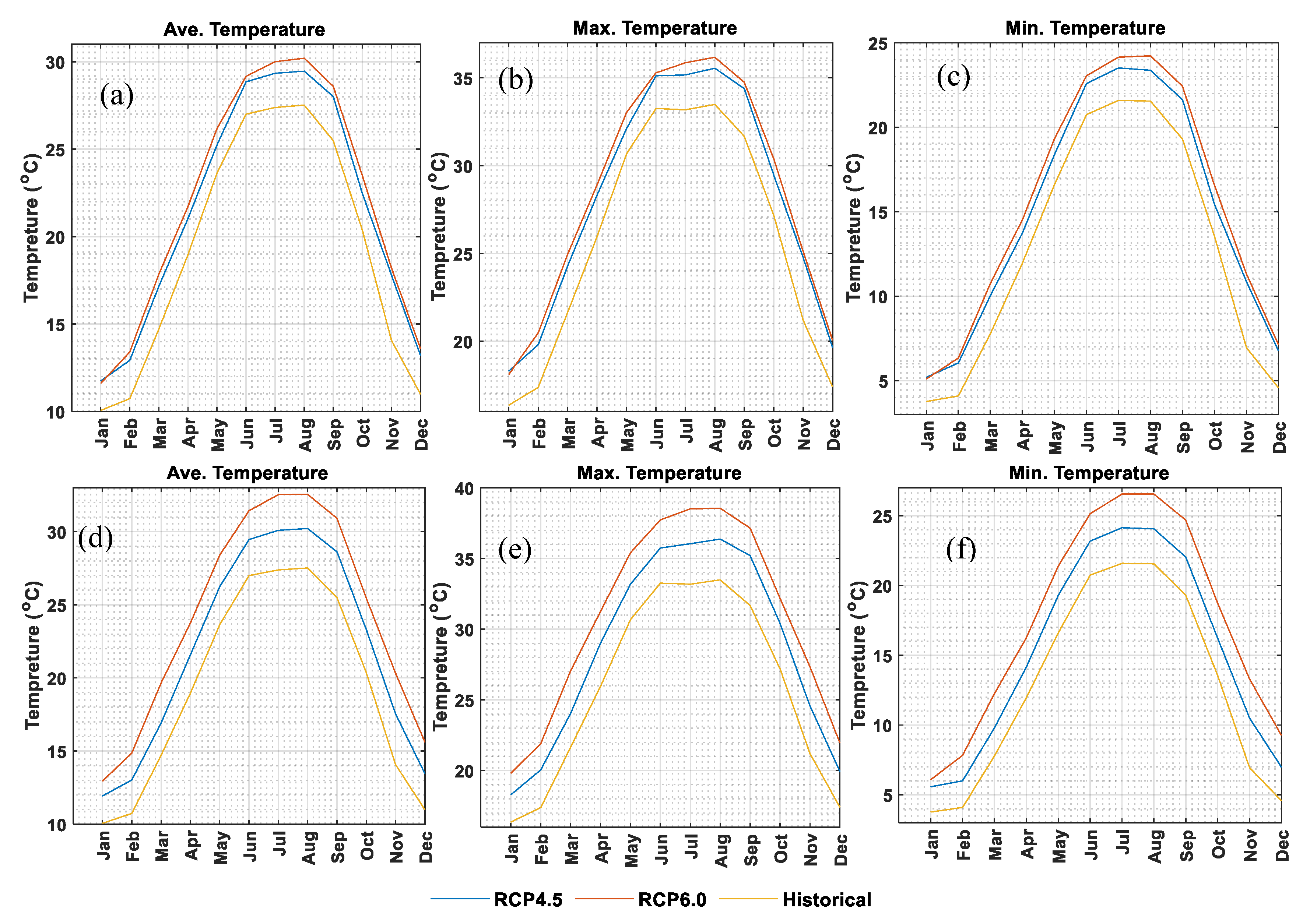
Average maximum and minimum temperature have important repercussions on hydrological implications.
Figure 4 represents monthly average of basin-wide daily maximum temperature (
Figure 4b), monthly average of basin-wide daily minimum temperature (
Figure 4c), and monthly average of basin-wide daily temperature (
Figure 4a). For average temperature (
Figure 4a), models match the observed average temperature, from mid-March to June (spring) and from mid-September to mid-November (fall). For winter (DJF) and summer (JJA), however, there are differences up to 1 °C. This trend is the same for maximum temperature (
Figure 4b) and minimum temperature (
Figure 4c). However, the discrepancies for maximum temperature during summer (the peak of the graph) and for minimum temperature during winter (the legs of the graph) are more noticeable. This behavior indicates that the more extreme the temperature, the bigger the difference between the models and the observed data.
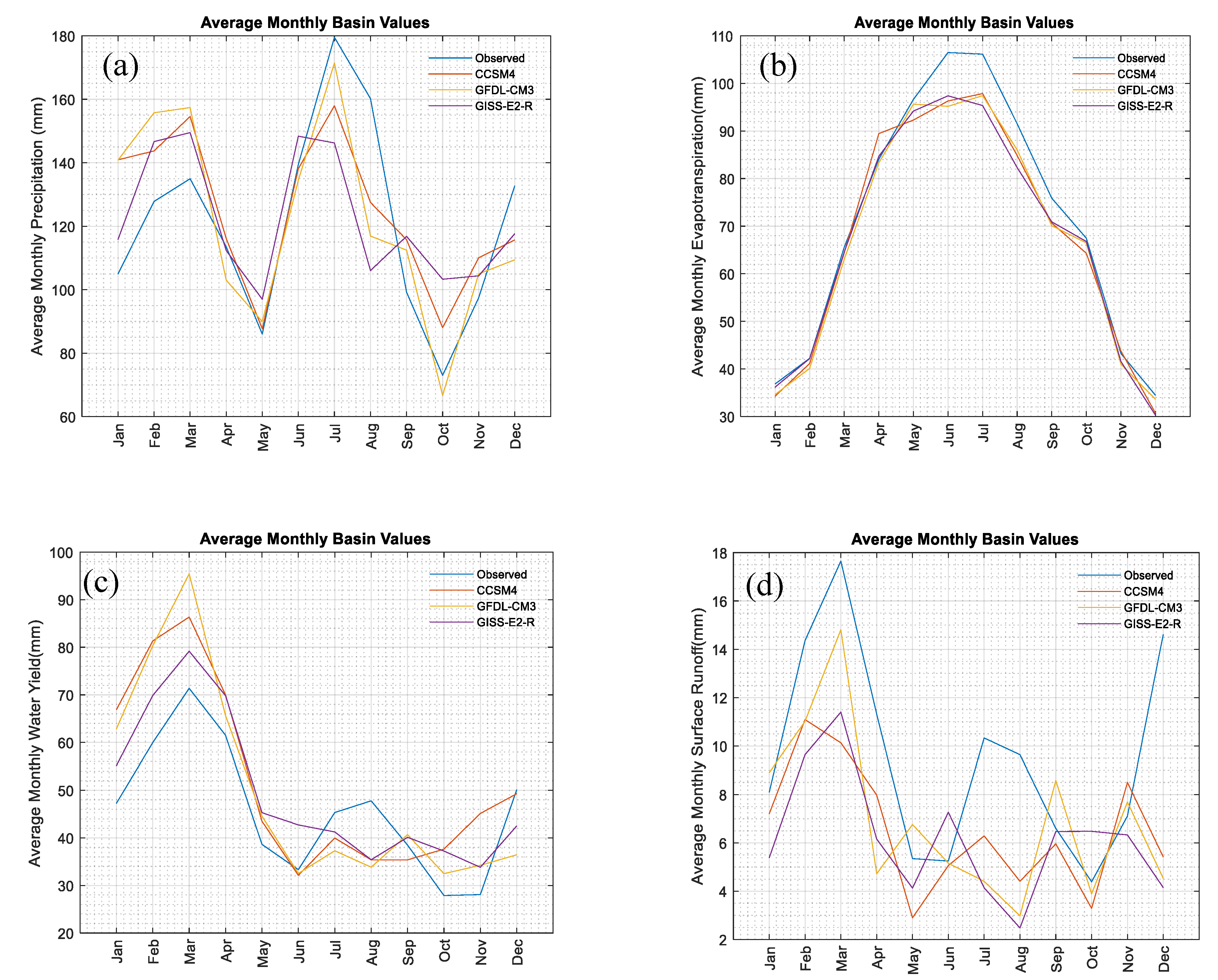
Figure 5 shows the monthly average of precipitation, ET, water yield, and surface runoff for 10 year for both the baseline and observed periods. From mid-March to mid-June and September and November, the average observed rainfall is the same as the models’ prediction with negligible differences. During summer and winter, however, there exist some discrepancies. These discrepancies could be attributed to the model biases. As SWAT model uses these model results as climate data, the biases can be projected to the simulated hydrological results such as ET, water yield, and surface runoff. Model predictions for ET (
Figure 5b) match with the observed data except during summer with small differences of up to 8% in July. The highest level of water yield occurs during the month of March (
Figure 5c) where the difference with the model prediction is around 13%. During spring, summer, and fall, the models predict an amount of average water yield close to the observed data. Since surface runoff amount and water yield are linked, the yearly pattern of surface runoff follows the water yield pattern. Surface runoff is underestimated. For example, in March when the highest amount of surface runoff happens through the year, the models’ predictions are 17% low for CCSM4 and GISS-E2-R and 11% low for GDFL-CM3. This difference is due to land use changes through the time period. Therefore, it indicates the biases of the land use map. In this study, we have not looked for extreme events that partially account for these biases. Thus, considering the different source of inevitable biases, it can be concluded that the results based on the models are reliable.
9. Annual and Seasonal Impacts of Future Climate on Water Regime
To obtain data required for future water regime, the CMIP5 multi-model ensemble LOCA was integrated with the SWAT model. We then derived precipitation, surface runoff, water yield, ET, and discharge for Bellwood (USGS2361500) monitoring point. We analyzed the data at monthly, seasonal, and annual scales.
Table 8 represents the projected mean annual changes to hydrological components for the entire simulation period and each decade. Mean annual change to the discharge at Bellwood station has an increase of 30.45% under the moderate scenario and 29.67% increase under the severe scenarios during the entire simulation period. Similarly, mean annual surface runoff during the period has significantly increased with 337.4% and 325.66% under moderate and severe scenarios, respectively ([
16,
18]). Water yield also has shown increases of 18.34% and 18.08% under moderate and severe scenarios through the entire period. Slight decreases of 0.8% under the moderate scenario and 2.46% under the severe scenario were observed to mean annual ET during the entire simulation ([
16,
20,
24]).
Table 8 presents the simulated mean annual changes to water balance components for mid-century and late-century periods. During the mid-century, mean annual discharge at Bellwood station was estimated to increase by 24.2% under RCP4.5 and 32.93% under RCP6.0. for the late century. However, the mean annual discharge at the station shows 36.72% increase under RCP4.5 and 26.4% increase under RCP6.0 ([
10,
15]). Under the severe scenario, despite the increased urbanization, the discharge amount at the station is projected to decrease towards the end of the century ([
24,
26]). It can be suggested that the last decade of water balance variables has been affected dramatically (
Table 8). Average annual surface runoff during the mid-century is estimated to increase by 286.3% under RCP4.5 and 315.5% under RCP6.0. Mean annual surface runoff continues to increase during the late century by an average of 388.5% under the moderate scenario and 335.9% under the severe emissions scenarios [
26]. These changes indicate the significant impact of the land use change on water balance variables [
22]. Increases to mean annual water yield were observed under both scenarios of moderate and severe emissions by 12.55% and 21.42% during the mid-century. During the late-century, average annual water yield is expected to increase by 24.14% under RCP4.5. For RCP6.0, however, average annual water yield is estimated to increase by 14.73% compared to the baseline period. Increase in mean annual water yield under RCP6.0 compared to the increase under RCP4.5 is much smaller during the late century. This is partially due to the dramatic drop in the hydrologic components during the 2090s [
18]. Unlike the other variables, slight decreases occur to mean annual ET during the mid- and late century. For the mid-century, a decrease of 0.63% and 0.01%, respectively, under the moderate and severe scenarios, is estimated. During the late-century, average annual ET decreases further with 0.95% and 4.92% under RCP4.5 and RCP6.0, respectively [
10].
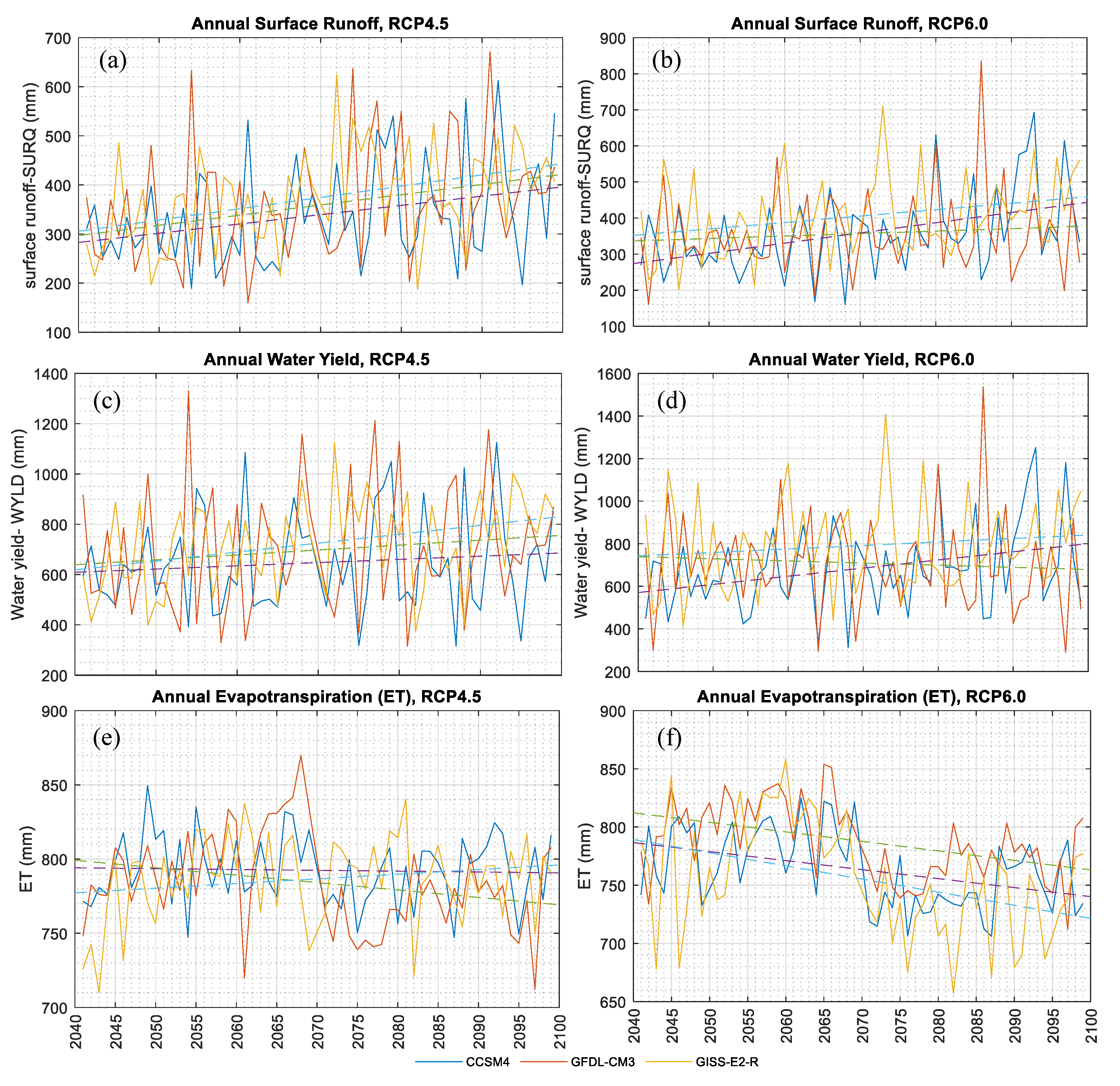
Figure 8 shows the mean annual trend of water balance variables (surface runoff, water yield, and ET) during the simulation period based on the models and under the scenarios. The regression lines for the surface under both scenarios indicate the increase during the entire simulation period. For water yield under the moderate scenario the regression lines for all models are slightly steep. The regression slope, however, increases under the severe scenario. The annual trend towards the end of the century shows an obvious decrease for ET under severe emissions scenarios ([
10,
12]).
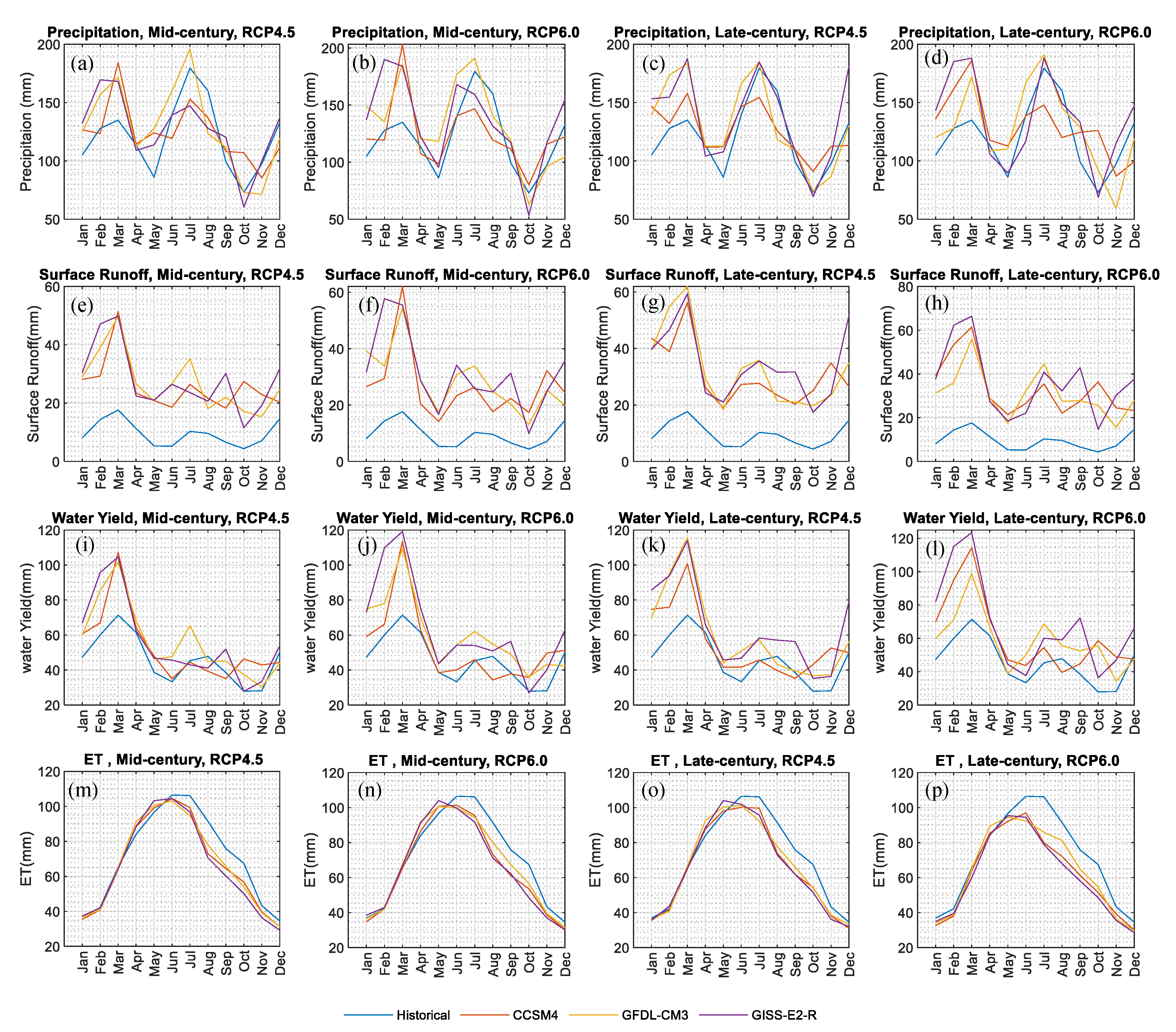
Basin-wide monthly average of the hydrological components is informative in investigating the water balance behavior of the watershed. The hydrological response to projected climate data in UCS changed for each month.
Table 9 and
Figure 9 illustrate these changes based on the models under both scenarios. During the mid-century, under moderate GHG emission, the largest change to precipitation is projected in May (during flooding season) with an increase of 48.5% compared to mean rainfall in the same month during the baseline period. For January, February, and March, it increases 18.9%, 22.6%, and 27.4%, respectively [
10]. The largest decrease in rainfall, however, is estimated in August and October with 23% and 26.7%, respectively (RCP4.5, Mid-century). During the late century under RCP4.5, the largest increase and decrease are projected in March with 36.1% and in August with 26.1%, respectively. For the severe emissions scenario, the largest rainfall increase and decrease during the mid-century are in January (41.8%) and December (21.1%), respectively. For the late century, however, precipitation decreases overall. The largest increase is expected to happen in September (29.9%) and the largest decrease in October (39.2%). Overall, August, October, and December are expected to be drier and January, March, and May are expected to be significantly wetter through the entire simulation period under both scenarios ([
12,
15,
17]). Similar to mean annual behavior of surface runoff, monthly estimates are also projected to increase dramatically [
26]. Under both scenarios, June has the highest increase of up to 5 times baseline period in monthly basin-wide surface runoff. The second highest increase is expected to happen in January with up to 4 times of the baseline period. The smallest increase in monthly mean surface runoff is projected in December with the lowest increase under RCP6.0 during the late century (36.2%) (
Table 9 and
Figure 9). Monthly behavior of water yield amount differs from rainfall and surface runoff [
25]. Under RCP4.5, overall water yield is projected to be higher than that of mid-century. The largest changes under the moderate scenario are estimated for February (+58.6%) and March (+62.1%) during the late century and in June (+42.9%) and July (+44.4%) during the mid-century (RCP4.5). Under the moderate scenario, water yield is estimated to decrease during the mid-century in December by 12.4% and in August by 6.3%. Mean water yield for each month indicates different behavior under the severe emissions scenario than expected. Under RCP6.0 and during the mid-century, January and June and October have increases of 58.4%, 62.7%, and 53.7%, respectively. Through the late century, however, November has the largest increase, 99.4%, in water yield amount. Under RCP6.0, water yield decreases only in December through the entire simulation period (
Table 9 and
Figure 9). Overall ET is expected to decrease slightly [
10]. For all months, mean ET drops except for April and May. Under both scenarios, the largest decrease is estimated in November with close to 20% drop. From
Figure 9, the level of decrease in ET during summer and fall can be easily distinguished. Monthly discharge projection is shown in
Figure 10 and
Table 9. Under both scenarios discharge is estimated to decrease in April and December at Bellwood station with the largest drop of 31.2% in December during the mid-century under severe emissions ([
9,
11,
30]). In other months, discharge is expected to increase. During the mid-century, the largest increase is observed in July (106.7%) and September (115.7%) under RCP4.5 and RCP6.0, respectively. During the late-century, February, July, and November have almost the same discharge under the moderate emissions. For the severe emissions conditions, however, September and November have the highest increases of 133.7% and 186.3%, respectively. The discharge projections indicate increases in the months in which rainfall is expected to decrease. This can be attributed to the land use change [
19].
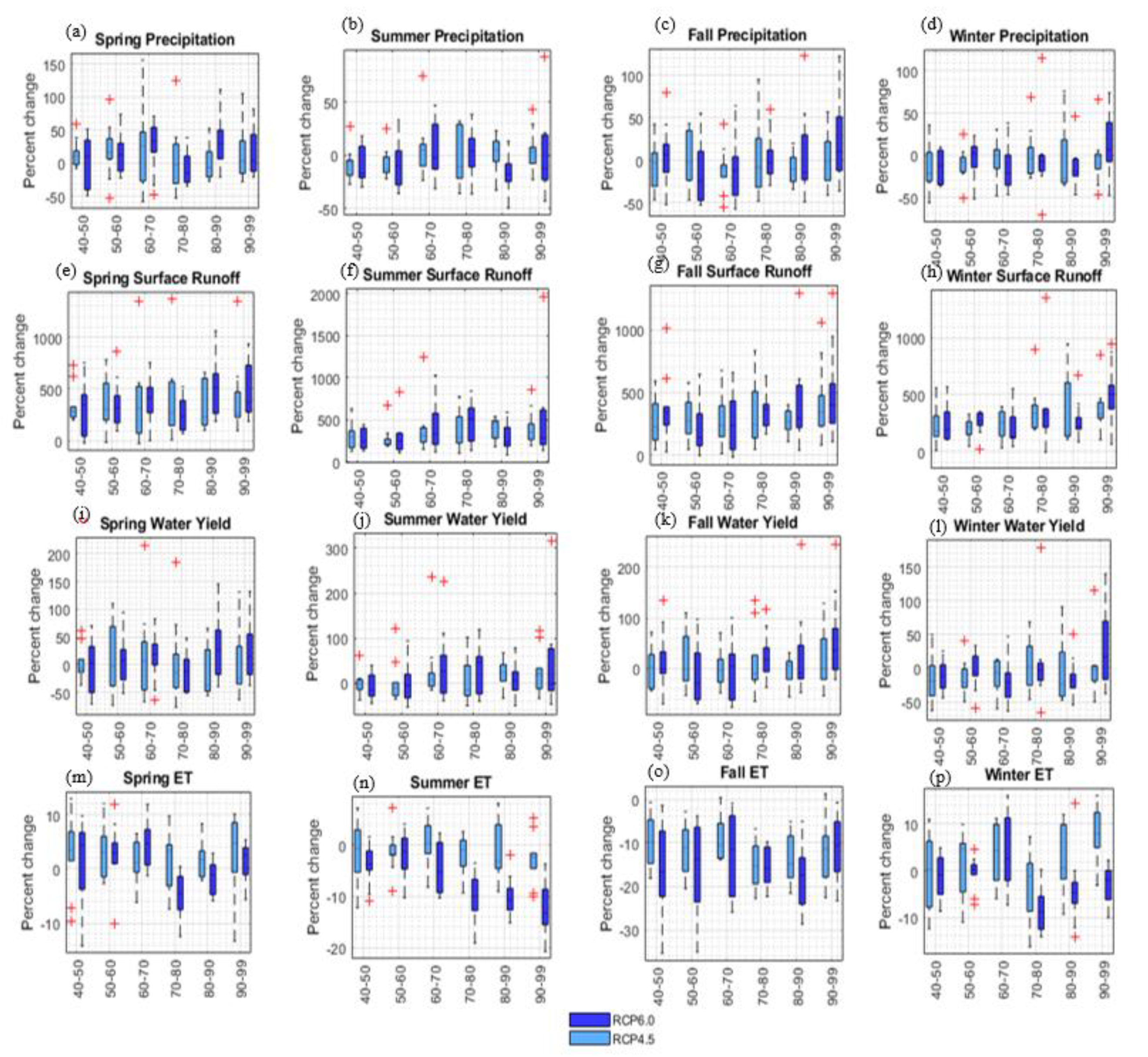
Seasonal variations are also expected in hydrological response to future climate data. Interquartile range (IQR) can be used to express this variability (
Figure 11). Outliers can be attributed to extreme weather [
35]. Moreover, larger IQRs indicate more frequent severe weather [
28]. The most frequent extreme rainfall in spring is expected during the 2060s under moderate emissions. These extreme behaviors, however, are expected two decades earlier (2040s) under severe emissions. Under moderate emissions, the 2050s have the wettest spring and the 2080s have the driest. Under severe emissions, the 2060s and 2070s have the wettest and driest spring, respectively (compared to the baseline period) ([
28,
129]).
IQR ranges for summer rainfall are noticeably smaller than those for spring, meaning smaller changes for summer rainfalls. Overall, IQR under RCP6.0 is longer indicating more under severe emissions. Moderate emissions, however, reflect more outliers indicating greater likelihood of heavy rainfalls during summer. Under RCP4.5, the 2070s and 2040s have the wettest and driest summers. Under RCP6.0, however, the 2060s and 2080s are expected to experience the wettest and driest summers ([
128,
129]).
Similar to summer rainfall, fall rainfall also has larger overall IQR under RCP6.0 than RCP4.5, indicating more changes under severe emissions. The smallest IQR ranging from −19.5% to −5.1% (under RCP4.5) is estimated during the 2060s where change variations indicate a noticeable number of outliers, meaning strong fall precipitations compared to the baseline period. A big portion of the 2090s’ IQR indicates increase, but for the 2050s a decrease is observed. This makes the end of the late century to have the wettest fall and the middle of the mid-century to have the driest fall (under RCP6.0) ([
28,
128]).
Projected winter rainfall has the shortest IQRs (smallest changes) compared to the other three seasons (in both emissions scenarios). For both scenarios, during the entire simulation period, IQRs and medians fall below the zero line, meaning decreased amount of precipitation during winter [
28]. The direst winter under severe emissions is projected for the end of the mid-century (60 s) where the median is −21.5%. Comparing the percent change variations for projected precipitation under both scenarios shows the largest changes in summer and winter when switching from RCP4.5 to RCP6.0. Similar results were observed by [
28].
Surface runoff variations show dramatic changes. For all seasons and under both scenarios, surface runoff is projected to increase up to several folds [
24]. For spring surface runoff, under RCP4.5, the largest IQR is expected by the end of the mid-century (2060s) ranging from 76.9% to 526.5%. Spring surface runoff, under RCP6.0, has an overall length of IQR shorter than that of RCP4.5, indicating less variations in percent changes. Comparison of spring surface runoff under both scenarios shows significant differences during the beginning of the simulation where moderate emissions make the shortest IQR while severe emissions make one of the largest variations. Through the entire simulation period, the overall IQR for summer surface runoff under RCP6.0 is larger than that of Rcp4.5, indicating more variations under severe emissions. For the fall surface runoff, the overall length for IQR varies through the simulation for both scenarios. The percent change values are also as high as spring’s and summer’s, indicating several fold surface runoffs. For winter surface runoff, the overall length of IQR under moderate emissions is greater than that of severe emissions, indicating more variation compared to the baseline period ([
26,
128]).
Water yield percent change variations indicates both increasing and decreasing amounts through all seasons [
34]. Since the surface runoff and water yield are related, water yield follows the same pattern as the surface runoff does, but due to affected partitioning, the level change differs ([
25,
26,
47]). For summer water yield, variations under RCP6.0 appear to be greater. This discrepancy is more obvious at the beginning and at the end of the simulation period. Under RCP4.5, the largest IQR, ranging from −28.7% to 38.8%, is projected at the beginning of the late-century period (2070s). RCP4.5 has resulted in more outliers than RCP6.0 indicating a higher chance of extreme amounts. For fall water yield, medians under both scenarios show mild changes towards the end the century. The overall length of IQR under RCP6.0 is longer than that of RCP4.5, indicating more variations under severe emissions. The largest IQR under RCP4.5 is estimated during 2050s (ranging from −24.6% to 63%). Under severe emissions, the largest variations are projected during 2050s ranging from −62.2% to 30.4%. Winter water yield projections indicate decrease during the mid-century period and slight increase by end of the century under both emissions scenarios [
23].
ET has the smallest changes and variations compared to other hydrologic variables during all seasons [
35]. Positive changes of ET during spring show general increase [
10]. Through the mid-century period, ET decreases (RCP4.5), while during the late century, it increases towards the end of the period. Under RCP6.0, during the late-century, decreases are observed, while RCP4.5 shows ET increases during the period. During summer, ET is expected to decrease always under RCP6.0. The largest (ranging from −4.6% to 3.9%) and the shortest (ranging from −1.99% to −0.02%) IQR are projected during the 2080s and the 2050s, respectively. ET during fall shows decrease for both scenarios and for the entire period. The projections indicate that the largest decrease is estimated during fall and under RCP6.0 up to −23.5% during the 2050s [
18]. Projection for ET during winter follows the same pattern as summer ([
13,
23]).
10. Implication of Future Water Regime
Here we integrated two types of projection: land use and climate data. Therefore, changes regarding land use and climate are the two main factors that affected the water regime [
26]. Results show consistency between the moderate and the severe emissions scenarios regarding the projected hydrological variables. Through the simulation period, precipitation increases; consequently, annual discharge increases. This increase is intensified by growing urbanization [
24]. Land use classes of URMD, URHD, and UIDU change from the mid-century period to the late-century period by 10%, 47%, and 12.5%, respectively. Therefore, even decreases of precipitation or attenuation in increase of rainfall towards the end of the century is compensated by more increasing impermeable land covers [
143]. These land use changes come along with a 23.1% decrease in forest cover (FRSE, FRSD, FRST), a 14.7% in hay cover (HAY) and a 11.8% in agricultural cover (AGRR). These changes affect regions’ microclimate impacting the water balance [
29]. RCP4.5 stabilizes atmospheric radiative forcing at 4.5 W/m
2 (650 ppm CO
2 eq) in 2100 ([
58,
68]); however, by the end of the mid-century period, the increase in the radiative forcing attenuates significantly. Unlike, RCP4.5, RCP6.0 keeps increasing by the end of the century and stabilizes the radiative forcing at 6.0 W/m
2 (850 ppm CO
2 eq); however, GHG emissions decline after the end of the mid-century period [
58]. Therefore, under RCP6.0, precipitation increases during the mid-century, and it declines during the late-century period. As a result, this decline is expected to be reflected in discharge amount, but urban-oriented land use change results in increased discharge ([
24,
26]). Similarly, surface runoff and water yield increase in the same manner. However, since discharge and water yield are linked to groundwater ([
46,
47,
144]), unlike surface runoff, they are indirectly affected. Surface runoff projection increases are significantly greater for all types of monthly, seasonal, and annual values. Annual results, for instance, show to be at least 3 times higher compared to the baseline. Similar studies have concluded the same result in the region ([
26,
28]). Increase in impermeable land covers (URMD, URHD, UIDU) decreases the amount of infiltration into the soil, and subsequently while baseflow contribution declines, surface runoff dramatically increases; this leads to more frequent and intense flooding ([
26,
145,
146]). Combined effects of increase in precipitation and temperature as well as imperviousness leads to a slight decrease in ET during the mid- and late century periods. Chen et al. [
21] have reported the same result. This indicates increased urbanization compensates for increased demand of evaporation and transpiration [
25]. Since, the vegetation and tree cover decrease under the land use scenarios, much less transpiration and plant uptake are estimated. It can be concluded that the increase in evaporation due to increase in urbanization cannot be offset by decrease in transpiration ([
24,
26]). Moreover, decline in soil water consumption and plant uptake due to less vegetation-covered lands can lead to increase in stream flow ([
28,
147]). Seasonal percent change analysis (
Figure 11) indicates that most dramatic changes (more frequent extreme situations) to climate and hydrological variables are projected at the beginning of the mid-century period when switching from moderate to severe emissions. Seasonal behavior also agrees with annual changes; however, it indicates more changes in winter and summer. Similar results were reported by Sunde et al. [
28] and Wang et al. [
26]. In a study ([
10]) for the entire southeast region, decline in storm water has been projected. The general increase in this study can be attributed to urban-oriented land use change as well as the watershed specific characteristics like seasonality and storm frequencies ([
28,
30,
31]).
Previous studies in the region have used CMIP3 or CMIP5 with general bias correction. CMIP5 with finer resolution and LOCA with more reliable climate data, now, have improved the future climate data projections ([
80,
148]). More realistic regional patterns of precipitation, better estimates of extreme events, and reduced number of light-precipitation days are the advantages of LOCA [
80]. These improvements have reflected more reliable results in this study. This study helped to fill the current need to investigate the combined effects of the most recent downscaled and bias-corrected climate projections and the land use projections based on SSP of IPCC. LUC scenarios used here are consistent with SSP and IPCC and couple improved demographic growth model with a spatial allocation model. There have been very few studies of this type investigating the integrated effects of projected land use and climate data on hydrological responses in the Southeast US on this study’s scale. UCS is mainly forested and agricultural which complicates the impacts and responses. More studies are required to investigate the combined effects of this type of watersheds where notable levels of humidity and proximity to the Gulf area which is exposed to more hurricanes and tropical storms affect the land use and hydrologic cycle. Wang et al. [
26] have studied an area close to UCS under CMIP3 and concluded the same results of this study. Because of the few number of research in the region where UCS locates and the also because of the approach used in this research, the result and projections brought here can be put into the overall research body and also can be served as a basis for comparison and decision making process. The approach also can be utilized for other watersheds to investigate the integrate the land use and climate projections to study the hydrologic response. A few Native American Reservations are located within UCS; therefore, this study can also be used to research the future climate impact on the reservations’ sustainability and the people. It should be noticed that we used SWAT weather generator to simulate wind speed, relative humidity, and solar radiation. The soil condition has not been changed, i.e., for all models the current condition was used. Models also had challenges predicting the monthly average temperature, monthly average of maximum temperature, and monthly average of minimum temperature for months of December, January, and in some cases February.


