Development of a SWAT Hydropower Operation Routine and Its Application to Assessing Hydrological Alterations in the Mekong

Abstract

Reservoir operations and climate change can alter natural river flow regimes. To assess impacts of climate and hydropower operations on downstream flows and energy generation, an integrated hydropower operations and catchment hydrological model is needed. The widely used hydrological model Soil and Water Assessment Tool (SWAT) is ideal for catchment hydrology, but provides only limited reservoir operation functions. A hydropower reservoir operation routine (HydROR) was thus developed for SWAT to analyze complex reservoir systems under different policies. The Hydrologic Engineering Center’s Reservoir System Simulation (HEC-ResSim) model, a well-established reservoir simulation model, was used to indirectly evaluate functionality of the HydROR. A comparison between HydROR and HEC-ResSim under a range of operation rule curves resulted in R² values exceeding 0.99. The HydROR was then applied to assess hydrological alterations due to combined impacts of climate change and reservoir operations of 38 hydropower dams in the 3S basin of the Mekong River. Hydropower production under climate change varied from −1.6% to 2.3%, depending on the general circulation model chosen. Changing the hydropower operation policy from maximizing energy production to maintaining ecological flows resulted in a production change of 13%. The calculation of hydrological alteration indices at the outlet of the 3S basin revealed that over 113% alteration in the natural river outflow regime occurred from the combined impacts of climate change and reservoir operations. Furthermore, seasonal flows and extreme water conditions changed by 154% and 104%, respectively. Alterations were also significant within the basin, and, as expected, were larger for high-head and small-river reservoirs. These alterations will adversely affect ecological dynamics, in particular, habitat availability. HydROR proved to be a valuable addition to SWAT for the analyses of complex reservoir systems under different policies and climate change scenarios.

1. Introduction

Hydropower reservoirs generate benefits by producing renewable energy that plays an essential role in the reduction of greenhouse gas emissions [1,2]. Currently, hydropower is one of the largest renewable electricity generation sources in the world. The total installed hydropower capacity worldwide has reached 1267 GW (Gigawatt) in 2018, generating 4185 TWh (Terawatt-hour), which accounts for 16% of the total electricity generated [3]. Hydropower is generated by converting potential energy into electricity. The water balance of the catchment determines the water inflows into a reservoir, and consequently affects the hydropower generation [4]. Hence, accurate simulation of catchment hydrology is essential for the management and operation of a reservoir.

A hydrological model mimics the real world system and is mainly used for predicting system behavior and for simulations of various hydrological processes [5]. Nowadays, hydrological models are considered essential tools for water resource management [6]. Hydropower reservoirs may alter the hydrologic regimes of rivers by shifting the seasonal flow patterns [7,8], by trapping sediments upstream of dams and by increasing the sediment transport capacity downstream of dams [9]. Hence the complex interaction of reservoir operations and natural hydrological processes must be captured. Examples of models that allow for reservoir operation simulations based on pre-specified rule curves include HEC-ResSim, the Water Rights Analysis Package (WRAP) modeling system and MODSIM. HEC-ResSim was developed by the US Army Corps of Engineers, Hydrologic Engineering Center, and is used to simulate reservoir operations at one or more reservoirs for various operational goals and constraints [10]. Applications include reservoir flood management, low flow augmentation and water supply for planning studies, detailed reservoir regulation plan investigations and real-time decision support [11]. The WRAP was designed for long-term, monthly time-step modeling assessments of hydrologic and institutional water availability and reliability for water supply diversions, environmental flow requirements, hydropower energy generation and reservoir storage [12]. MODSIM is a generic river basin management decision support system, originally conceived in 1978 at Colorado State University [13], making it the longest continuously maintained river basin management software package currently available from an open source. MODSIM considers hydropower reservoir operation by including reservoir balancing routines, allowing division of reservoir storage into several operational zones for controlling the spatial distribution of available storage in a river basin [14].

Despite the existence of models for the simulation of hydropower reservoirs, these have limited applicability in complex catchments to concurrently simulate flows, the water balance and sediment transport for changing climate and land use. This is particularly relevant as land management, climate and land use change impact surface runoff, shift seasonal flow patterns, alter dry and wet periods and change sediment fluxes, which eventually affects reservoir operation [15,16,17,18,19,20].

One hydrological model which has a basic built-in reservoir routine is the Soil and Water Assessment Tool (SWAT). SWAT is a physically-based hydrological model initially developed to assess stream flows, sediment yield, chemical yield and nutrient processes in large watersheds [21]. SWAT is extensively used around the world and it has been used to various levels of success in catchments in which hydropower development is ongoing [22,23,24,25,26]. However, SWAT lacks the capability to model complex hydropower reservoir operations and energy generation. To better understand the complex effects of hydropower operations on downstream flows, current applications in catchments have focused on externally linking SWAT with models such as HEC-ResSim [10]. This linked approach, however, is complex to set up and does not allow for simulating climate change and land use change impacts on reservoir operations simultaneously.

In this paper, the development, testing and implementation of a new SWAT hydropower reservoir operation routine (HydROR) to simulate hydropower reservoir operations, energy generation and their effects on flows downstream is presented. In an example application of SWAT with the HydROR, climate change impacts on energy production and hydrologic alterations due to reservoir operations were assessed for the Sesan, Srepok and Srekong (3S) sub-basins of the Mekong basin. The Mekong basin is the second most biodiverse region in the world [27], which includes 781 fish species [28]. The exceptional fisheries in the basin are dependent on river flows [29] and the annual natural flood pulse is the main driving factor of the high biodiversity [28,30]. The basin is undergoing rapid development and the riparian countries have been planning extensively to construct large reservoirs in the main stream, and along the tributaries of the Mekong [31]. These developments could alter the natural flow regime of the basin. Therefore, in this study, we applied the HydROR specifically to quantify hydrological alterations due to reservoir operations in the 3S basin.

2. Development of a Hydropower Reservoir Operation Routine for SWAT

2.1. SWAT Model

The Soil and Water Assessment Tool (SWAT) [21] is one of the ecohydrological models for the river basin scale which was developed in the early 1990s by the U.S. Department of Agriculture, Agricultural Research Service (USDA-ARS) [32,33]. Since then, SWAT has been continuously improved, capabilities have been added and it has been applied worldwide in water resources. The model was chosen for this work due to its versatility and the fact that the source code and extensive documentation are available in the public domain.

SWAT is a conceptual model that operates on a daily time step and can predict the impacts of land management practices on water, sediment and agricultural chemical yields (nutrient loss) in large and complex catchments with varying soils, land uses and management conditions over a long period of time [34]. Major components of the model are weather, hydrology, sedimentation, soil temperature, crop growth, nutrients, pesticides, bacteria and algae land management practices [34,35]. In the SWAT model, a river basin is divided into sub-basins, which are then further subdivided into hydrologic response units (HRUs) consisting of unique combinations of land use and soil characteristics based on topography. Various routines can be used to compute the relative impacts of land use, soil and weather within each HRU.

2.2. Existing Reservoir Routine in the SWAT

In SWAT, a reservoir, either man-made or naturally occurring, is an impoundment located on the main channel of the river system [34]. SWAT provides functions to account for the mass balance of water and sediment transported into and out of a reservoir [36]. A typical reservoir has an emergency spillway to control large floods safely and a principal spillway for frequent flood control. The reservoir outflow is determined based on the reservoir water balance:

$$V=V_{stored}+V_{flowin}-V_{outflow}+V_{pcp}-V_{evap}-V_{seep}$$

(1)

where V is the volume of water in the reservoir at the end of the simulation step (m³), V_stored is the volume of water stored in the reservoir at the beginning of the simulation step (m³), V_flowin is volume of water entering in the reservoir (m³), V_outflow is volume of water flowing out of the reservoir (m³), V_pcp is volume of precipitation falling on the reservoir (m³), V_evap is volume of evaporated water from the reservoir (m³) and V_seep is volume of water lost from the reservoir by seepage (m³).

The SWAT reservoir routine allows the user to determine V_outflow with one of four different methods: measured daily outflow, measured monthly outflow, average annual release rate for uncontrolled reservoir and controlled outflow with target release (Figure S1) [34]. In the measured daily or monthly outflow method, the reservoir outflow (V_outflow) is determined using time series data of daily or monthly outflow rate provided by the user. Contrarily, in the average annual release rate method, the reservoir releases water whenever the reservoir volume exceeds the principal spillway volume of the reservoir. In the target release method, the reservoir releases water as a function of the target storage and defined non-flood season [37]. In this way, the existing SWAT reservoir routine was primarily developed for those reservoirs which have adequate measured outflow data. In addition, SWAT allows one to simulate flood control reservoirs just accounting two flood limit levels and monthly flood storage, and it is especially suitable only for small reservoirs. Thus, the applicability of SWAT for highly-regulated, large-scale reservoirs with hydropower generation capacity is limited. In order to address this limitation, we developed a new algorithm for the SWAT reservoir routine to simulate hydropower reservoirs under predefined complex operational rules.

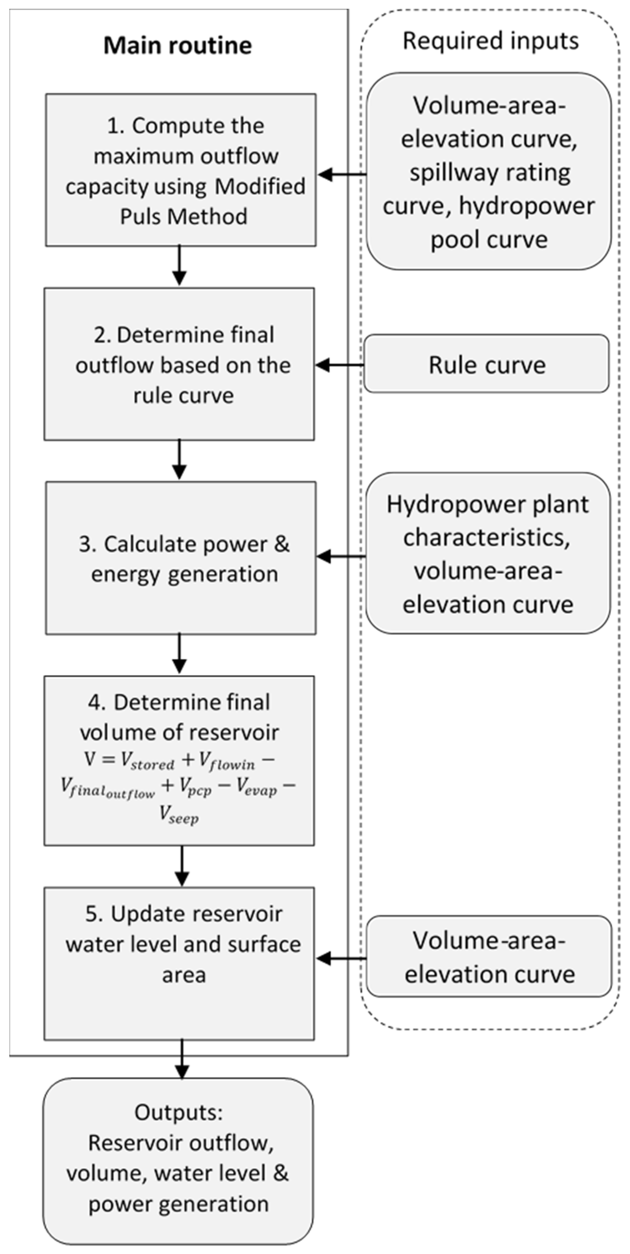
2.3. Hydropower Reservoir Operation Routine (HydROR)

A new hydropower reservoir operation routine (HydROR) was developed and integrated into SWAT. In the HydROR, the reservoir considered is a manmade structure and specifically used to generate hydropower and it replaces the existing simplified reservoir routine of the SWAT model. HydROR calculates the water balance of a reservoir and the energy generation of a hydropower plant using predefined rule curves and plant efficiency. Inflow to the reservoir, precipitation on the reservoir water surface, seepage loss and potential evapotranspiration from the reservoir are computed using existing SWAT routines.

In addition to data required for SWAT, area-elevation, volume-elevation curve, maximum/minimum operating levels, rule curves, outlet capacity curves, plant efficiency, installed capacity, headloss coefficient and design flow of the hydropower scheme must be provided by the user. These data are readily available from hydropower scheme operators. The main function computes outflows of a reservoir using reservoir routing and rule curves. The water balance equation (Equation (1)) is applied to calculate the water volume of the reservoir.

In step 1 (Figure 1), reservoir routing is calculated using the level pool routing method (modified Puls method), which estimates the maximum outflow capacity (V_outflow) of the reservoir by solving the continuity equation [38]. The V_outflow includes outflows from all the outlets at the simulation step. The relationship between reservoir volume, water level and outflow is established as a lookup table, combining an outflow rating curve and volume-elevation curve of the reservoir. This relationship table is used to estimate the maximum outflow capacity of the reservoir. Thus, the volume-elevation curve and the outflow rating curve (spillway rating curve) data of a reservoir must be provided for each reservoir in the basin considered. The relationship between water level and reservoir volume can be derived using topographic information of the reservoir. The outflow rating curve of a spillway is derived from hydraulic equations relating discharge and head of the spillways.

In step 2 (Figure 1), the final outflow (Equations (2)–(5)) of the reservoir is determined based on the operating policy using a user-defined rule curve of the reservoir because reservoirs have to be operated under various operational constraints and design restrictions. These constraints and restrictions are translated into a set of rule curves for the guidance of reservoir operators [39]. In HydROR, the rule curve is defined by specifying a target water level for the first day of each month and the routine calculates daily target water levels by linear interpolation.

$$V_{check}=V_{stored}+V_{flowin}+V_{pcp}-V_{evap}-V_{seep}-V_{rule}$$

(2)

$$\mathrm{IF}\left(V_{check}\le 0\right),\mathrm{then}{V}_{final\_outflow}=0$$

(3)

$$\mathrm{IF}\left(V_{check}\le V_{outflow}\right),\mathrm{then}{V}_{final\_outflow}=V_{check}$$

(4)

$$\mathrm{IF}(V_{check}>V_{outflow}),\mathrm{then}{V}_{final\_outflow}=V_{outflow}$$

(5)

where $V_{rule}$ is volume of the reservoir as indicated by the rule curve for a simulation time step and $V_{check}$ is the difference in total water volume (V) and $V_{rule}$. $V_{final\_outflow}$ is the final outflow from the reservoir. This final outflow includes the outflows from different outlets of a reservoir:

$$V_{final\_outflow}=V_{spill}+V_{tur}$$

(6)

where $V_{final\_outflow}$ is the final total outflow in terms of volume of water during the day (m³), $V_{spill}$ is the volume of water spilling from spillway in a day (m³) and $V_{tur}$ is the volume of water through turbine for power generation (m³). The discharge through a spillway is allocated using the outflow rating curve of the spillway. The turbine flow for hydropower generation depends on the design discharge for hydropower plants and operation rules.

In step 3 (Figure 1), power generation from the hydropower plant for every time step of simulation is calculated as in Equations (7) and (8).

$$P=\frac{\eta \times \gamma \times Q_{tur}\times H_{net}}{1000}$$

(7)

$$E=\frac{P\times \mathsf{\Delta }t}{1000}$$

(8)

where Q_tur is the flow through turbine in m³/s, η is the efficiency of power plant, γ is the specific gravity of water in KN/m³, H_net is net head for power plant in m, ∆t is time step in hour, P is power production in MW and E is energy generation in GWh. The net head is calculated by taking the difference between reservoir water level and the tailrace level/turbine level of the power plant, which should be entered by a user.

In step 4 (Figure 1), the HydROR updates reservoir water volume using the mass balance equation and updates water level and surface area from the volume-area-elevation curve of the reservoir. Finally, in step 5 (Figure 1) the outputs (reservoir volume, level, outflow and power generation) are written to an output file.

2.4. Evaluation of the HydROR

In order to test the performance of HydROR, the HEC-ResSim (Hydrologic Engineering Center’s reservoir system simulation) model [10], which was specifically designed by the U.S. Army Corps of Engineers, Hydrologic Engineering Center, to simulate multipurpose reservoirs, was used as a benchmark model for comparison and set up utilizing the same runoff data generated by the SWAT model. The Yali reservoir (one of the oldest reservoirs in the 3S basin) was selected to compare HydROR with HEC-ResSim for the time period between 1986 and 2008. Yali is located in a tributary of the Sesan River in Vietnam, about 70 km upstream of the border with Cambodia (Figure S2). The total catchment area at the Yali reservoir is 7445 km² and the dam operates between 515 m.a.s.l. to 490 m.a.s.l., with a maximum power generating capacity of 720 MW.

2.4.1. SWAT with HydROR and HEC-ResSim Model Simulation

The SWAT model of the Yali reservoir consists of one sub-basin and one HRU to illustrate a simple model setup and output analysis. The input data for the SWAT model includes one land use type, one soil layer, topography (digital elevation map) and daily weather data. Additional data which are essential for the application of SWAT with HydROR and HEC-ResSim include the volume-area-elevation curve, hydroplant pool curve, spillway rating curve, rule curve and hydropower plant characteristics (design discharge, minimum operating level, full supply level, installed capacity, tailwater/turbine level, plant efficiency, headloss coefficient) (Figure S3 and Table S1).

In addition to input flow from SWAT, the operation of a reservoir is primarily determined by the rule curve. Both HydROR and HEC-ResSim always attempt to bring the level of the reservoir as close as possible to the rule curve by obeying the operation rules.

The rule curve used for both HydROR and HEC-ResSim (Figure S3d) is typical of tropical seasonal systems, with the ability to release water in the wet season and fill the reservoir during the dry season. When the reservoir level is below the level of 490 m.a.s.l. in the month of June, the hydropower station stops producing energy, and when the water level is greater than 515 m.a.s.l., the reservoir starts spilling all the excess volume of water [40].

2.4.2. Performance Criteria

The criteria of goodness for fit of the model were evaluated by comparing the outputs of the HydROR routine and the HEC-ResSim model with respect to outflow, reservoir water level and power generation. Nash–Sutcliffe efficiency (NSE) [41], which has been widely used in water resources to assess the performance of a hydrological model [42], was used to evaluate the performance and is given by:

$$\mathrm{NSE}=1-\frac{{\sum }^{\text{}}{\left(Q_h-Q_{\mathrm{s}}\right)}^2}{{\sum }^{\text{}}{\left(Q_h-{\overline{ Q}}_h\right)}^2}$$

(9)

where $Q_h$, $Q_s$ and ${\overline{Q}}_h$ are the outflow from HEC-ResSim model, outflow from HydROR and average outflow from HEC-ResSim model in m³/s respectively. The NSE can vary from −∞ to 1, whereby the 1 is the perfect fit of the model.

Moreover, the performance of HydROR was evaluated by the ratio of standard deviation of observations to root mean square error (RSR) [43].

$$\mathrm{RSR}=\frac{\sqrt{{\sum }^{\text{}}{\left(Q_h-Q_s\right)}^2}}{\sqrt{{\sum }^{\text{}}{\left(Q_h-\overline{Q_h}\right)}^2}}$$

(10)

The percent bias (PBIAS), a method to measure the average tendency of the simulated values to be larger or smaller than their observed values [44], was used as well.

$$\mathrm{PBIAS}=\frac{{\sum }^{\text{}}\left(Q_h-Q_s\right)}{{\sum }^{\text{}}\left(Q_h\right)}\times 100$$

(11)

3. Application of the HydROR

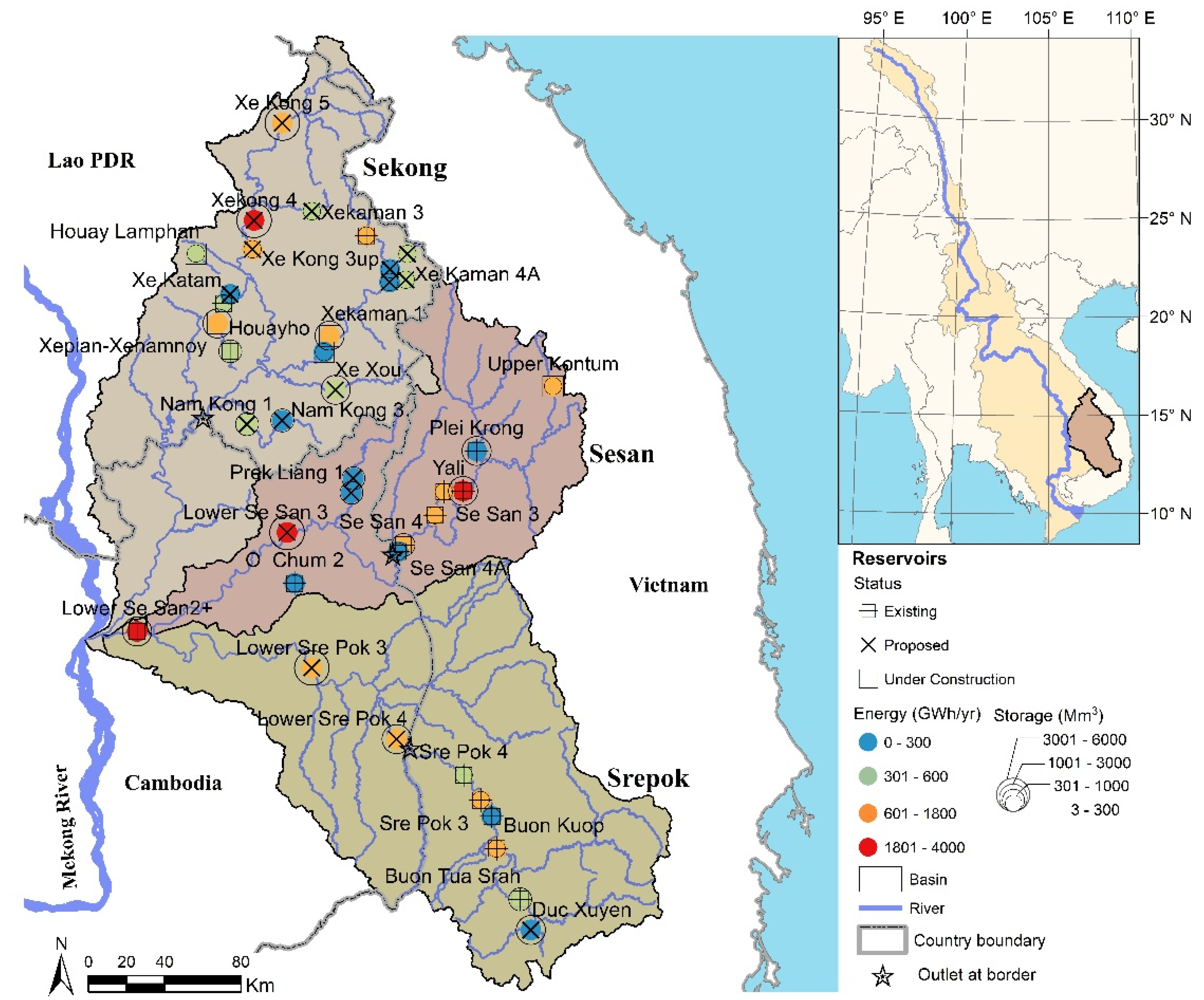
Following the comparative performance of HydROR with HEC-ResSim for a single reservoir, a multi-hydropower simulation of the 3S sub-basin of the Mekong basin was conducted with HydROR to demonstrate its capacity for dealing with complex scenarios.

3.1. Study Area

The Mekong is the largest trans-boundary river basin in Southeast Asia, with a catchment area of 795,000 km², discharging 475 km³ of water annually [45]. Originating from the Tibetan Plateau, the river flows through China, Myanmar, Laos, Thailand, Cambodia and Vietnam (Figure 2). The 3S rivers (Sekong, Sesan and Srepok), are the largest tributary system, thereby contributing about 20% of flow to the lower Mekong basin. The catchment area of the 3S basin is 78,650 km², of which 33% is situated in Cambodia, 29% in Lao PDR, and 38% in Vietnam. Energy demand has begun to sharply increase in the Southeast Asian region since 2000 due to growing populations, rising incomes, rapid urbanization and easy access to energy [46]. Therefore, currently hydropower reservoirs in the 3S basin are being planned and developed at a fast pace to fulfill the increasing energy demand [45]. In this study, we considered 38 hydropower projects (Figure 2) to investigate climate change impacts on energy production and to quantify hydrological alterations due to operation of these reservoirs. We selected hydropower projects according to their status of progress (existing, under construction, proposed), size, location, installed capacity, development priority and data availability (Table S2).

3.2. Hydrological Modelling

A calibrated and validated SWAT model of the 3S basin [22,45,47,48,49] was used for the HydROR application. Input data were obtained from the Information and Knowledge Management Programme, Mekong River Commission (MRC, an inter-governmental organisation which jointly works with the governments of Cambodia, Lao PDR, Thailand and Vietnam to manage the sustainable development of the water resources of the Mekong River) [47]. The datasets used for the SWAT model were a digital elevation model (DEM) map of 250 × 250 m resolution; land use types information and a land use map; a soil map; and daily precipitation, maximum and minimum temperature, solar radiation, wind velocity and relative humidity data. The SWAT model for 3S basin was calibrated and validated for the period 1985 to 2000 and 2001 to 2007 for observed daily discharge (Figures S4 and S5, Tables S3 and S4) respectively (for details see [47]).

3.3. Hydropower Reservoir Simulation

HydROR has the capability to simulate complex systems of multiple hydropower reservoirs in a river basin under predefined rule curves. In this study two types of rule curves were employed: (1) the seasonal variation (SV) rule curve and (2) the full supply level (FSL) rule curve. The seasonal variation rule curve was set to optimize energy production, storing water during the wet season to allow for extended generation during the dry season. On the other hand, the FSL rule curve aims to keep the reservoir at its full supply level to simulate a more natural to ecological flow regime downstream. It allows for the release of water for generation when the water level is higher than FSL and fills the reservoir when water level is lower than FSL.

3.4. Climate Change Scenarios

To assess the impacts of climate change on hydropower production in the 3S basin, we selected three general circulation models (GCMs), i.e., the Goddard Institute for Space Studies Model E2, coupled with the Russell ocean model, with carbon cycle (GISS-E2-R-CC); the Institute Pierre-Simon Laplace Coupled Model, version 5A, coupled with NEMO, mid resolution (IPSLCM5-MR); and Geophysical Fluid Dynamics Laboratory Climate model version 3 (GFDL-CM3). Furthermore, three emissions scenarios of representative concentration pathways (RCPs), RCP2.6 (low emissions), RCP6.0 (medium emissions) and RCP8.5 (high emissions) (Table S5), were selected from the four resource concentration pathways developed for the IPCC 5th Assessment Report [50]. These GCMs and emissions scenarios were selected because previous studies demonstrated that these models are reasonable for simulating the most influential climate processes in the monsoon region [47,51]. The period 2051–2070 was chosen for analyzing the climate change impacts for the 3S basin. Previous studies [47,51] indicate that this period can provide a better representation of the development of hydropower projects in the 3S basin. In this study, we applied the climate change projections dataset of monthly change factors, which are readable by SWAT model, for precipitation, temperature, solar radiation and relative humidity provided by the MRC Climate Change and Adaptation Initiative (CCAI). The method used to downscale the climate change projections dataset is described in [47].

3.5. Analyzing Changes Using Indicators of Hydrological Alternation (IHA Method)

The IHA (indicators of hydrological alteration) were developed by a group from The Nature Conservancy to assess impacts of human activities (e.g., reservoir operations, flow diversion or channel irrigation) on flow regimes [52]. The IHA software package computes 33 hydro-ecologically-relevant parameters based on the pre-impact and post-impact periods of streamflow data. The IHA parameters are classified into five groups characterizing the hydrologic regime with respect to magnitude of monthly flow, magnitude and duration of annual extreme events, timing of annual extremes, frequency and duration of high and low pulses and rate of change in water conditions (

Table 1. The 33 indicators of hydrologic alteration (IHAs) adapted from IHA Manual V7 [52,53,59,60].

IHA Parameters Group	Hydrologic Parameters	Ecosystem Influences
Group 1. Magnitude of monthly water conditions (12 IHAs)	Mean or median discharge for each calendar month (m3/s)	Provide availability of habitat, soil moisture, water and food; access by predators to nesting sites; functional link to water temperature, oxygen levels, photosynthesis
Group 2. Magnitude and duration of annual extreme flows, and the base flow condition (12 IHAs)	Annual 1-, 3-, 7-, 30-, 90-day minimum flow (m3/s)	Creation of sites for plant colonization; structuring of river channel morphology and physical habitat conditions; nutrient exchanges between rivers and floodplains; distribution of plant communities in lakes, ponds and floodplains
	Annual 1-, 3-, 7-, 30-, 90-day maximum flow (m3/s)
	Number of zero days
	Base-flow index (m3/s)
Group 3. Timing of annual extreme flow conditions (2 IHAs)	Julian date of annual 1-day minimum	Provide special habitats during reproduction or to avoid predation; influences spawning for migratory fish, evolution of life history strategies
	Julian date of annual 1-day maximum
Group 4. Frequency and duration of high and low pulses (4 IHAs)	Number of low pulses each year	Connection to soil moisture and anaerobic stress for plants; Provide floodplain habitats; ensure nutrient and organic matter exchanges between river and floodplain, soil mineral availability Influences bedload transport, channel sediment textures and duration of substrate disturbance (high pulses)
	Mean duration of low pulses (days)
	Number of high pulses each year
	Mean duration of high pulses (days)
Group 5. Rate and frequency of flow changes (3 IHAs)	Rise rate	Drought stress on plants (falling levels), Entrapment of organisms on islands, floodplains (rising levels), Desiccation stress on low-mobility stream edge (varial zone) organisms
	Fall rate
	Number of reversals

) [52,53].

Generally, observed hydrological data are used to calculate IHA parameters by dividing data period into pre-dam and post-dam periods. However, getting reliable long-term hydrological data at downstream dam sites is difficult [54]. Using simulated data is thus the next logical choice, particularly for understanding the cumulative impacts of climate change and operation of reservoirs on hydrological alterations [18,55,56,57,58].

In this study, we used these 33 IHA parameters to quantify changes in the hydrologic regime due to reservoir operations and selected climate change scenarios. For every downstream dam (Figure 2), mean values of each IHA parameter were calculated for both pre and post-impact periods. The pre-impact flow data, which represent the natural flow regime, were obtained from SWAT simulation runs without reservoir operations using historical climate data for the period 1986–2005. The post-impact flow data were determined by simulating reservoir operations and climate change scenarios with HydROR for the period 2051–2070. We then calculated hydrological alteration (HA) values for each parameter using the following equation [59]:

$$\mathrm{HA}\%=\frac{M_{Post}-M_{pre}}{M_{pre}}\times 100$$

(12)

where M_post is the mean for the post-impact period and M_pre is the mean for the pre-impact period. In addition, HA values were averaged by parameter groups and for all parameters.

3.6. Scenarios

Considering existing, under construction and planned hydropower reservoirs in the 3S basin, GCMs and emissions scenarios, we developed a set of scenarios to assess the impacts of climate change on hydropower production, as shown in

Table 2. Description of scenarios to assess impacts of climate change on hydropower production.

Scenarios	Name	Climatic Condition		Period
Baseline (no reservoirs)	BL	Historical climate		1986–2005
Baseline (with reservoirs)	BLR
Climate change (no reservoirs)	GISSL	Goddard Institute for Space Studies Model E2, coupled with the Russell ocean model, with carbon cycle (GISS-E2-R-CC)	RCP2.6	2051–2070
	GISSM		RCP6.0
	GISSH		RCP8.5
	IPSLL	Institute Pierre-Simon Laplace Coupled Model, version 5A, coupled with NEMO, mid resolution (IPSL-CM5A-MR)	RCP2.6
	IPSLM		RCP6.0
	IPSLH		RCP8.5
	GFDLL	Geophysical Fluid Dynamics Laboratory Climate model version 3 (GFDL-CM3)	RCP2.6
	GFDLM		RCP6.0
	GFDLH		RCP8.5
Climate change (with reservoirs)	GISSLR	Goddard Institute for Space Studies Model E2, coupled with the Russell ocean model, with carbon cycle (GISS-E2-R-CC)	RCP2.6
	GISSMR		RCP6.0
	GISSHR		RCP8.5
	IPSLLR	Institute Pierre-Simon Laplace Coupled Model, version 5A, coupled with NEMO, mid resolution (IPSL-CM5A-MR)	RCP2.6
	IPSLMR		RCP6.0
	IPSLHR		RCP8.5
	GFDLLR	Geophysical Fluid Dynamics Laboratory Climate model version 3 (GFDL-CM3)	RCP2.6
	GFDLMR		RCP6.0
	GFDLHR		RCP8.5

. The baseline (BL) scenario does not consider reservoirs and uses the observed historical climate data for the time period from 1986–2005. Most of the existing reservoirs have been constructed after 2000 and it is assumed that by 2051 all hydropower projects selected here will be operational. Furthermore, we outlined scenarios for reservoir operations under the baseline climate (BLR) and for three GCMs under three emissions scenarios (Table 2). These climate change scenarios, the GISS (“drier overall”), IPSL (“increased seasonality,” i.e., drier dry season and wetter wet season combined) and GFDL (“wetter overall”) model along with three emissions scenarios, were specifically proposed by the MRC [51] to assess climate change impacts on different sectors, such as domestic and industrial water consumptions, irrigation, hydropower and flood control in the Mekong basin. Therefore, these scenarios were outlined to comprehensively understand the impacts of climate change on hydropower production. Additionally, we used two types of rule curves—(1) the seasonal variation (SV) and (2) the full supply level (FSL) rule curve—for reservoir operations. The SV rule curve attempts to store water by reducing spillage during wet/flood season and release water during dry season for energy production. Thus, the main objective of the SV rule is to maximize energy production. In contrast, the FSL rule curve keeps the water level as high as the FSL of the reservoir. Thus, the reservoir acts as a run-of-the-river scheme and has the capability to maintain the downstream flow regime.

4. Results

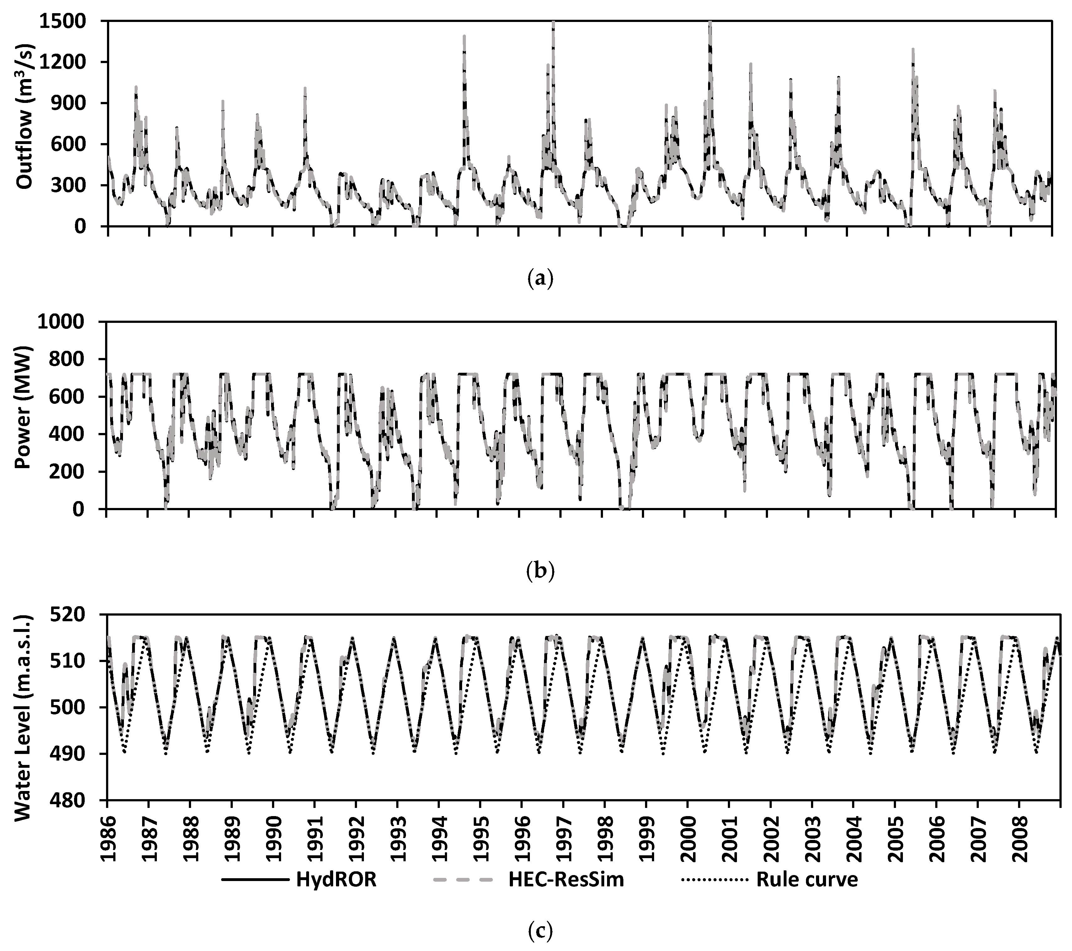
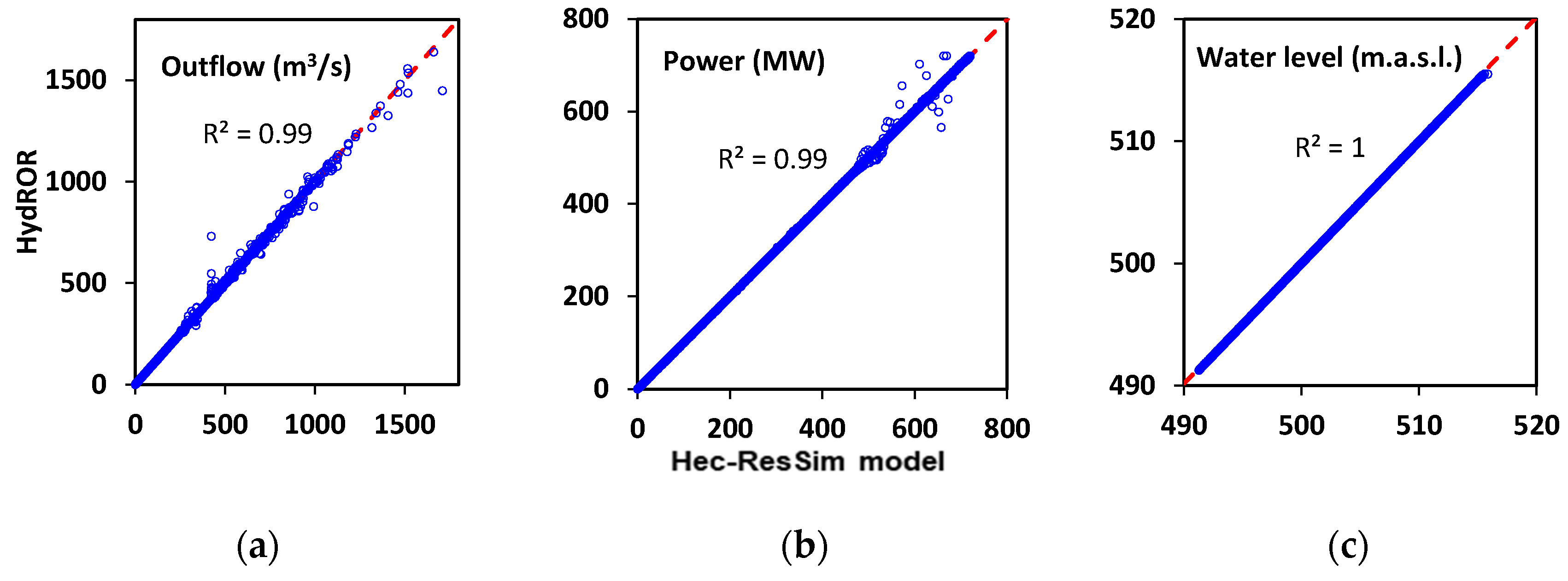
4.1. Performance of HydROR

A comparison of simulated outflows from the Yali hydropower reservoir between HydROR and HEC-ResSim models shows an excellent fit for outflows, power production and water levels with NSE and R² values exceeding 0.99, and RSR and PBIAS values lower than 0.01 (Figure 3 and Figure 4), confirming that the new routine reproduces the HEC-ResSim results. The disagreement in some instances stems from the different interpolation methods used by the two models. HydROR and HEC-ResSim reproduce the operation of the reservoir equally well, as shown in Figure 3c when simulated water levels are compared to a given input rule curve. In this study, we have set the HEC-ResSim as a benchmark model to evaluate the capability of the HydROR, because previous studies [11,40,48,61,62] have shown that the HEC-ResSim can simulate hydropower reservoirs according to imposed operating rule curves, predefined constraints and goals. The HydROR, like HEC-ResSim, requires the user to enter physical properties of hydropower plants, outlet capacities, reservoir geometry and operation policies (rule curves) to realistically simulate power generation and water releases.

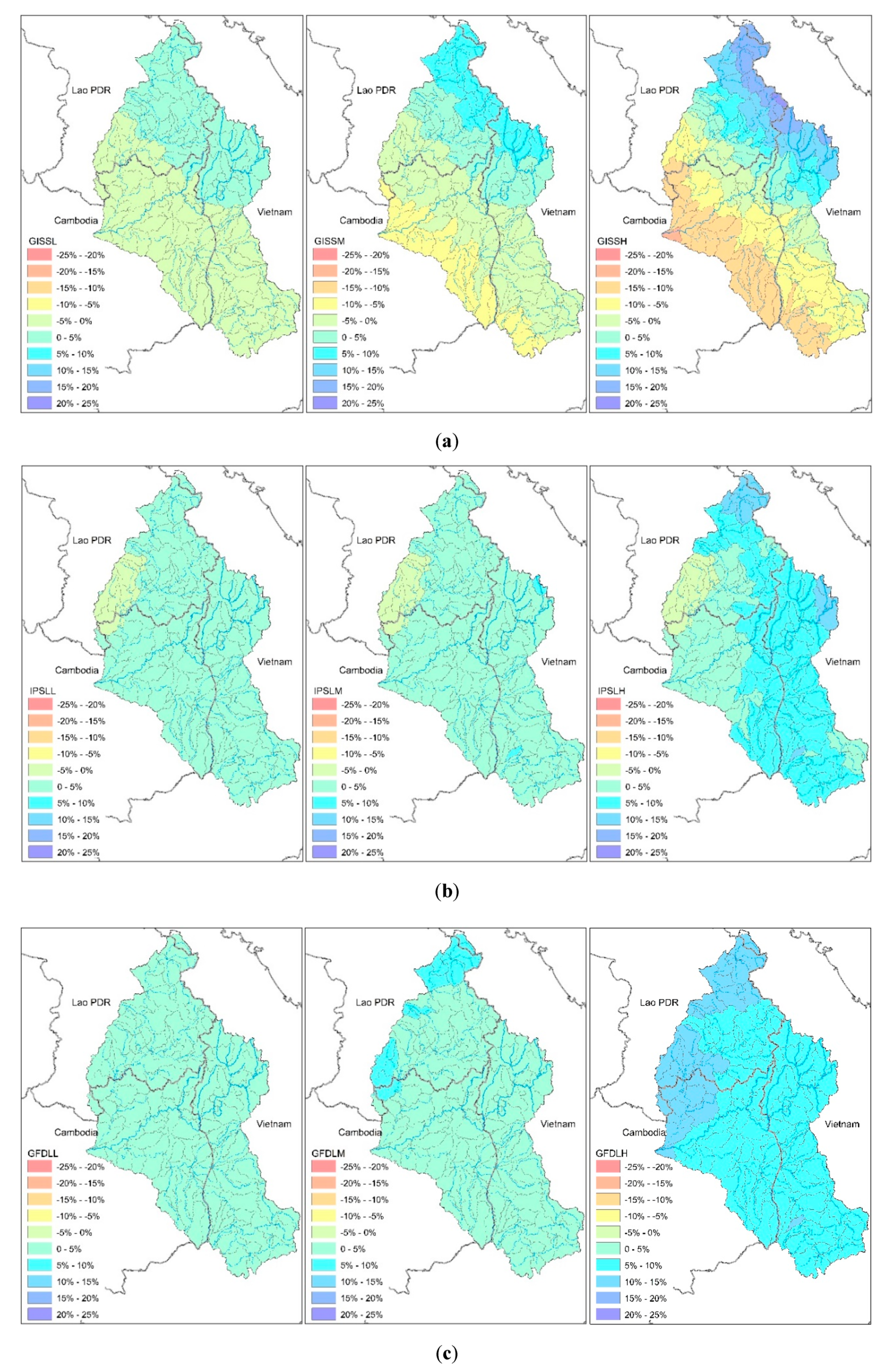
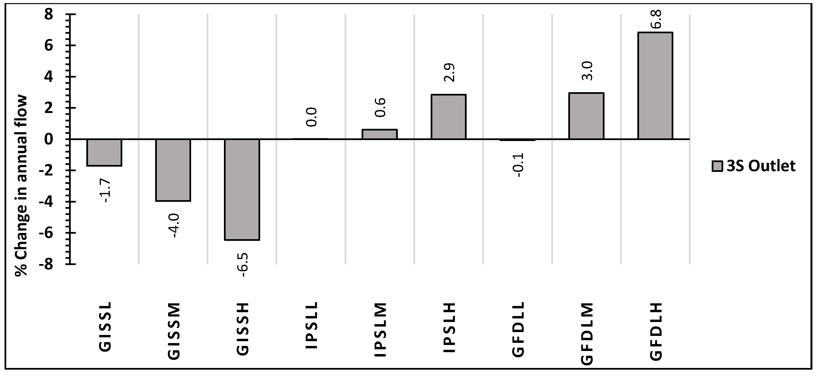
4.2. Climate Change Impacts on Precipitation and Flow

Annual average precipitation changes for the three GCMs and three emissions scenarios (L, M, H) with respect to the baseline period for the 3S basin showed significant spatial variation (Figure 5). According to the GISS model scenarios, annual precipitation will decrease up to 15% in the northeastern part of the 3S basin (most of that area lies in Lao and Vietnam) and will increase up to 20% in the southwestern part of the 3S basin (most of those areas lie in Cambodia). Average annual precipitation will increase up to 10% for the IPSL model scenarios, with strong spatial variations, depending on the emissions scenario. Similarly, the GFDL model scenarios also point to an increase in precipitation by 0.5–12%, yet the spatial distribution of the change in precipitation across the basin is the opposite to the distribution in the IPSL model’s results. Overall average annual changes in precipitation are −0.8%, 2.8% and 4.5% under the GISS, IPSL and GFDL models for the 3S basin respectively, indicating rather low impact of climate change on the annual precipitation amount at the basin level.

The change in average annual streamflow from various GCMs (for low, medium and high emissions) at the outlet of the 3S basin is shown in Figure 6. The results indicate that average annual flow decreases by 6.5% for the GISS model for the high emissions scenario and increases for both IPSL and GFDL models, with a maximum increase of 6.8% at the 3S outlet.

The GCMs exhibited variation in annual precipitation among the sub-basins. This resulted in a predicted increases in annual flows under the IPSL and GFDL (for medium and high emissions) models and decreases in annual flows under the GISS model, which are in agreement with previous studies [63] of climate change projections in the lower Mekong basin. Uncertainties associated with GCMs should not be neglected [47].

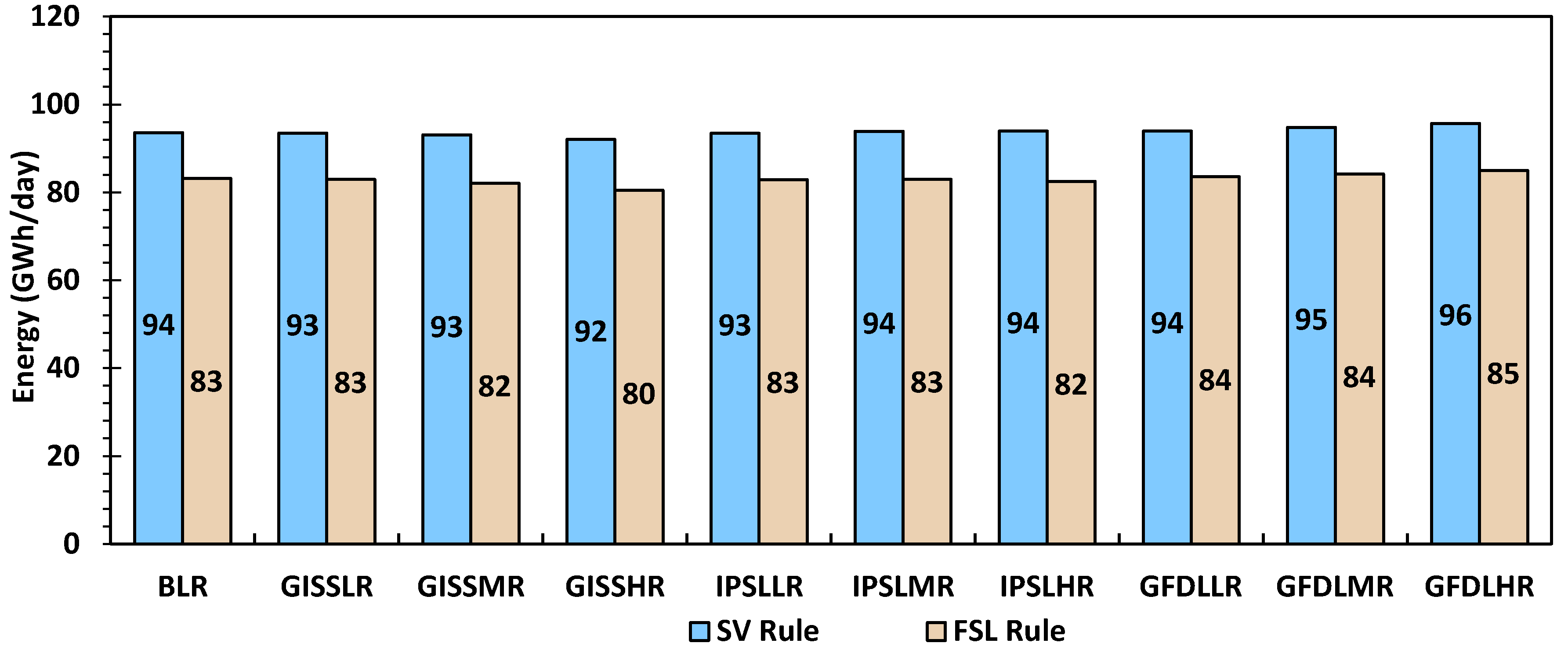
4.3. Impacts of Operation Rules and Climate Change on Hydropower Production

The average daily hydropower production levels from all reservoirs for the baseline climate scenario with the seasonal variation (BLR-SV) rule and full supply level (BLR-FSL) rule curves are 94 and 83 GWh, respectively, i.e., an 11% difference (Figure 7 and Table S6).

For the climate change scenarios investigated here, the average energy production decreases slightly for the GISS model for all emission scenarios when compared with the BLR scenario, whereas the energy production slightly increases for the GFDL model for all emissions scenarios. The energy production varies for the IPSL model for different emissions scenarios. The maximum increase in energy production is 2.3% for the GFDL model (high emissions scenario) and the maximum reduction in energy production is 1.6% for the GISS model (high emissions scenario). The average hydropower production for the 3S basin decreased 0.7% for the GISS model, and increased 0.2% and 1.3% for the IPSL and GFDL models, respectively.

The combined consideration of climate change scenarios and different rule curves revealed that energy production varies between 11% to 13% for the three GCMs, three emissions scenarios and SV and FSL rule curves (Table S7).

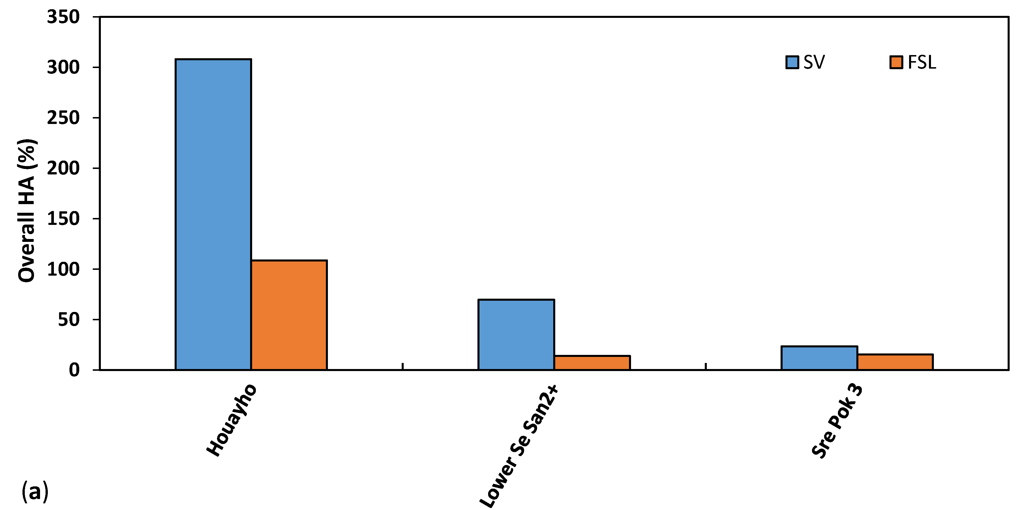
4.4. HA Due to Reservoir Operation and Climate Change

An alteration in the hydrologic regime can be observed downstream of all reservoirs. However, the magnitude and nature of the impact vary considerably by the reservoir, operation rule and climate change scenario. The mean overall HA from baseline conditions is 102% under the SV rule, with the highest value of 308% and the lowest value of 16% for specific reservoirs (Figure 8a). The reservoirs in the Xe Kong River, a tributary of the Se Kong River, have high HA values (highest value for the Houayho hydropower scheme), whereas reservoirs in the Sesan sub-basin (except for Upper Kontum) and the Srepok sub-basin have comparably low HA values under the SV rule (Figure S6 and Table S8). The lowest impact results from the Xe Kaman 4A reservoir in the Sekong sub-basin.

Amongst all reservoirs, the most significant alterations of hydrologic regime occurred in groups 1 and 4 (Figure 8b) of HA parameters, which are related to the mean monthly flows and frequency/duration of high and low pulses.

The ratio of HA to simulated hydropower generation in GWh per year (Figure 8c) represents the impact of reservoirs in terms of energy production. The Xe Nam Noy 5, Namkong 3 and Xekaman-Sanxay hydropower schemes show the highest HA to energy production ratios, whereas Yali hydropower scheme shows the lowest ratio (Figure S6c).

The result shows that HA values due to reservoir operations under the FSL rule curve were lower than under the SV rule curve (Figure 8a), with overall HA values of 109%, 14% and 15% for the Houayho, LSS2 and Srepok 3 reservoir respectively. Furthermore, we found a maximum overall HA value of 114% for Duk E Mule and a minimum value of 1% for both the Prek Liang 2 reservoir and Xe Kaman 4A reservoir (Figure S7 and Table S9). The overall HA values decrease up to 99% under the FSL rule curve compared to the overall HA value under the SV rule curve (Figure 9). Similarly, group HA parameters and HA/GWh values also decreased for most of the reservoirs. An increase in groups 4 and 5 HA parameters for some of the reservoirs under the FSL rule curve (Figure 8b) was observed. The results show an increase in HA/GWh value for the lower Sesan 3 reservoir. This was due to the significant decrease (20%) in energy production under the FSL rule curve. The mean overall HA across all reservoirs was 28% (Figure 10) under the FSL rule curve, which is 73% less than under the SV rule curve. Yet, the overall HA values for the Duc Xuyen reservoir increased due to the increase of group 4 HA parameters as a result of a significant increase in low flood pulse frequency. In general, HA values under the SV rule curve are higher than under the FSL rule curve due to the cumulative impact of hydropower operations, and HA values are even large when considering high emissions climate change scenarios (Figure 10).

4.5. Predictors for Alteration

The design head of the hydropower plants and active storage height of the reservoirs in the 3S basin are positively correlated with HA values, whereas mean flow of the river and design discharge of hydropower schemes are negatively correlated with HA for the SV and FSL rule curves (

Table 3. Pearson correlation R values for overall HA and individual IHA parameter groups (Group 1–5 IHA parameters are denoted as Gr1–5) among logarithmic predictor values for features (Energy: annual energy production; Installed: installed capacity; Storage: reservoir storage capacity at full supply level; Area: reservoir surface area at FSL; Act Ht: active storage height; FSL: full supply level; Head: design head of the scheme; Qmean: mean annual flow of the river and Qd: design discharge of the scheme) for the 3S basin under the SV-rule curve and FSL-rule curve (green and red indicate positive and negative correlations, bold values represent p < 0.05).

SV Rule							FSL Rule
Feature	Overall	Gr 1	Gr 2	Gr 3	Gr 4	Gr 5	Overall	Gr 1	Gr 2	Gr 3	Gr 4	Gr 5
Energy	0.12	0.06	0.13	−0.06	0.10	0.20	0.13	0.16	0.15	0.07	0.00	0.02
Installed	0.12	0.09	0.02	−0.13	0.21	0.19	0.11	0.14	0.12	0.04	−0.02	0.08
Storage	0.22	0.17	0.20	−0.11	0.04	0.45	0.21	0.12	0.22	0.11	0.18	0.15
Area	0.17	0.17	0.10	−0.09	0.03	0.49	0.24	0.10	0.23	0.13	0.26	0.15
Act Ht	0.35	0.33	0.19	0.21	0.19	0.07	0.25	0.24	0.20	0.24	0.09	0.40
FSL	0.27	0.29	−0.07	0.32	0.44	−0.17	0.24	0.26	0.11	0.30	0.08	0.38
Head	0.49	0.44	0.18	0.38	0.45	0.11	0.31	0.41	0.28	0.41	−0.06	0.40
Qmean	−0.52	−0.54	−0.10	−0.39	−0.46	−0.03	−0.36	−0.37	−0.29	−0.38	−0.06	−0.59
Qd	−0.27	−0.26	−0.10	−0.37	−0.18	0.04	−0.12	−0.20	−0.10	−0.28	0.10	−0.24

and

Table 4. Pearson correlation R values for overall HA and IHA parameter groups (Group 1–5 IHA parameters are denoted as Gr1–5), between logarithmic predictor values for features (all notations are described in the caption of Table 3) for the (a) Sekong, (b) Sesan and (c) Srepok sub-basin under the SV-rule curve and FSL-rule curve (green and red indicate positive and negative correlations, bold values represent p < 0.05).

SV Rule							FSL Rule
(a)
Feature	Overall	Gr1	Gr2	Gr3	Gr4	Gr5	Overall	Gr1	Gr2	Gr3	Gr4	Gr5
Energy	0.37	0.22	0.35	−0.22	0.29	0.10	0.07	0.13	0.09	−0.06	−0.11	0.05
Installed	0.26	0.24	0.08	−0.33	0.35	0.12	0.06	0.11	0.03	−0.08	−0.09	0.19
Storage	0.53	0.47	0.27	−0.10	0.36	0.47	0.30	0.14	0.28	0.13	0.46	0.30
Area	0.56	0.52	0.24	−0.08	0.38	0.51	0.30	0.11	0.30	0.15	0.49	0.34
Act Ht	0.18	0.19	0.01	0.14	0.21	0.13	0.28	0.30	0.20	0.26	0.11	0.21
FSL	0.00	0.12	−0.32	0.29	0.29	−0.03	0.36	0.53	0.29	0.45	−0.17	0.25
Head	0.26	0.31	−0.09	0.33	0.43	0.02	0.45	0.59	0.34	0.48	−0.03	0.33
Qmean	−0.15	−0.35	0.40	−0.28	−0.47	−0.06	−0.50	−0.59	−0.41	−0.45	−0.05	−0.50
Qdesign	−0.01	−0.08	0.18	−0.51	−0.15	0.09	−0.36	−0.47	−0.26	−0.50	0.01	−0.17
(b)
Feature	Overall	Gr1	Gr2	Gr3	Gr4	Gr5	Overall	Gr1	Gr2	Gr3	Gr4	Gr5
Energy	0.16	0.14	−0.03	0.16	0.15	0.23	0.28	0.40	0.42	0.19	0.12	−0.10
Installed	0.16	0.14	−0.21	0.27	0.25	0.20	0.34	0.42	0.43	0.20	0.18	0.00
Storage	0.05	0.29	0.49	0.10	−0.23	0.23	0.36	0.41	0.45	0.03	0.16	0.26
Area	−0.10	0.14	0.10	0.44	−0.21	0.55	0.59	0.77	0.74	0.60	0.27	0.23
Act Ht	0.14	0.28	0.01	−0.07	0.11	−0.30	0.16	0.19	0.27	−0.36	0.02	0.35
FSL	0.58	0.45	−0.21	0.20	0.67	−0.56	0.08	−0.26	−0.20	−0.71	0.17	0.37
Head	0.72	0.58	0.16	0.17	0.62	−0.07	−0.18	0.04	0.10	−0.40	−0.25	−0.06
Qmean	−0.77	−0.64	−0.17	−0.15	−0.68	0.55	0.34	0.54	0.49	0.86	0.16	−0.22
Qdesign	−0.21	−0.12	−0.21	0.19	−0.12	0.19	0.55	0.38	0.36	0.37	0.44	0.07
(c)
Feature	Overall	Gr1	Gr2	Gr3	Gr4	Gr5	Overall	Gr1	Gr2	Gr3	Gr4	Gr5
Energy	−0.01	−0.14	0.43	−0.23	−0.44	0.46	−0.52	0.32	0.28	−0.27	−0.53	−0.45
Installed	0.08	0.14	0.55	−0.13	−0.31	0.46	−0.31	0.05	0.01	−0.13	−0.35	−0.27
Storage	0.76	0.71	0.72	0.37	0.26	0.68	0.28	−0.24	−0.22	0.09	0.29	0.29
Area	0.76	0.70	0.83	0.16	0.00	0.85	0.14	−0.10	−0.09	0.06	0.14	0.13
Act Ht	0.65	0.39	−0.35	0.83	0.61	−0.23	0.56	−0.60	−0.56	−0.18	0.56	0.79
FSL	−0.02	0.16	−0.69	0.59	0.69	−0.78	0.67	−0.54	−0.50	0.24	0.68	0.68
Head	0.04	0.06	−0.16	0.28	0.27	−0.22	0.18	−0.04	−0.03	0.14	0.18	0.10
Qmean	−0.24	−0.14	0.71	−0.60	−0.82	0.69	−0.89	0.35	0.28	−0.31	−0.80	−0.70
Qdesign	−0.06	−0.20	0.46	−0.34	−0.57	0.50	−0.67	0.28	0.22	−0.45	−0.67	−0.47

). Furthermore, the design head is a significant predictor of HA in parameter groups 1, 3 and 4 for the SV rule curve and in parameter groups 1, 3 and 5 under the FSL rule. However, reservoir surface area and storage capacity are dominant predictors of overall HA for the Sekong and Srepok sub-basin for both rule curves (Table 4a,c). Yet for the Sesan sub-basin, HA values are significantly correlated with design head for the SV rule curve and with the reservoir surface area for the FSL rule curve. The average streamflow (Qmean) is negatively correlated to the overall HA for all three sub-basins, except for the Sesan sub-basin when the FSL rule curve is considered. The regression analysis showed a spatial dependence of the predictors of alteration for the three sub-basins. The reservoir surface area is highly correlated with alterations for the Sekong and Srepok sub-basins, whereas this is not the case for the Sesan sub-basin. Reasons for this may be the differing topography and hydro-climatic conditions.

5. Discussion

5.1. Impacts of Climate Change on Hydropower Production

The daily hydropower production in the 3S basin varies from 92 to 96 GWh under various climate change scenarios, which represents a −1.6% to +2.3% change from the baseline scenario. Yet overall, the impact of climate change on hydropower production is insignificant in the 3S basin for the 2051–2070 period, as the reservoir operations overcome the impact of climate change on the flows.

5.2. HA Due to Reservoir Operations and Climate Change

Analysis of the hydrological alterations parameters shows that flow regime alteration is likely due to the operation of reservoirs. However, the magnitude and intensity of the alterations vary widely based on reservoir characteristics, location and operation policies, which has also been pointed out in other studies [58,59,60,64,65,66]. Our results indicated that, in addition to reservoir features, the location of the reservoir is also a significant factor for variations of the rate of hydrologic alterations, as the basin is characterized by wide variation in topography and physiography with complex climatic conditions.

We found that the most significant changes occur for monthly flow volume, and magnitude and duration of extreme annual flow (IHA parameter groups 1 and 2). Reservoir volume, area and design head of the hydropower scheme showed more sensitive to IHA parameter groups 1 and 2. That was all due to the operation of the reservoirs under the SV rule, and is in agreement with previous work [48,67,68,69]. More specifically, dry season flow (November–April) substantially increased and wet season flow (May–October) decreased due to reservoir operation, because reservoirs store water during the wet season and release water to generate hydropower energy in the dry season. Overall, alterations were observed to a lesser degree for the wet season when compared to the dry season.

The results show a significant increase in annual minimum flows and a decrease in annual maximum flows due to operation of hydropower reservoirs, which aligns with previous findings in this region [23,70]. The HA values of group 3 parameters indicate an alteration in the timing of annual extreme water conditions. The values of these group parameters were larger for reservoirs that are located on small rivers, i.e., rivers which have relatively low mean flows. This was because small-river reservoirs delayed the timing of annual maximum flows. However, HA values of group 3 are comparatively lower than the HA values of groups 1 and 2. Furthermore, impacts of reservoir operations on flood pulse dynamics, which are presented by IHA parameter group 4, are relatively lower than HA in group 1, although the Houayho, Upper-Kontum, Duc Xuyen, Se San 3A, Se San 3, Buon Tua Srah and Yali reservoirs show high HA values of group 4. HA values of groups 4 and 5 indicate dam operations where operators store water to achieve sufficient head before releasing water for generating electricity during the dry season.

In addition to reservoir operations, climate change is another factor that can alter the dry seasonal flows and the flood pulse of the 3S rivers [69,71,72,73]. Piman et al. (2015) [73] projected a dry seasonal flows increase of 96% and a wet seasonal flows decrease of 25% due to the operations of 41 reservoirs at the 3S basin outlet. The same authors also predicted a dry seasonal flows reduction of 6–24% and indicated uncertainty in a change of wet seasonal flows due to climate change. Ngo et al. (2018) [72] forecasted that the annual flow might decrease by a 3–8% for the Sesan sub-basin and increase by a 4–13% for the Srepok sub-basin due to climate change, whereas reservoir operations alone might increase dry seasonal flow by 30% to 40% and wet seasonal flows might drop by 15% to 20% for the Sesan sub-basin. In an earlier modelling attempt, Lauri et al. (2012) [71] projected annual Mekong River discharge changes of −10% to +13% due to climate change, and a larger increase in dry seasonal flow (25–160%) and a decrease in wet seasonal flow (5–24%) due to reservoir operations. Variations in the modelled values of percentage changes relative to the results presented here are due to differences in the extent of the study area (i.e., whole of Mekong vs. 3S basin), the selection of projected hydropower projects, GCMs, the simulation period, operation policies and simulation models.

Overall, we found that the cumulative impacts of reservoir operations and climate change are more sensitive to the magnitude and duration of extreme flow conditions for the 3S basin. In addition, our study confirms that reservoir operations appear to have a considerably stronger impact on the flow regime than climate change [72,73,74]. Furthermore, land use change plays a major role in hydrological alterations [75], but in this study we have limited the analysis of impacts to reservoir operations and climate change.

Operating rule curves play an essential role in enhancing power production and to reduce impacts on the ecohydrological system downstream [76]. We used the FSL rule because previous studies [48,77] demonstrated that the application of this type rule has a low impact on the hydrological regime. In comparison with the SV rule, the application of FSL rules resulted in a significant overall decrease in HA (Figure 8). Additionally, decreases in HA values of groups 1 and 2 indicate that application of the FSL rule has low impacts on the flow regime. However, HA values of group 4 for Xe Xou, Duc Xuyen and Buon Tua Srah increased when using FSL rule curves, as explained by an observable increase in the low flood pulse. The designed discharges of these hydropower reservoirs are relatively larger than the mean monthly flow of the river. Thus, these reservoirs have the capacity to release larger amounts of water under the FSL rules during low flood season. Simulations under the FSL rule curve showed a decrease in energy production for all reservoirs, as expected, except for the Xe Kaman 2B, Houayho, Plei Krong, Duc Xuyen and Buon Tua Srah reservoirs which are relatively small and located uppermost of the cascades (Table S6). In general, however, the operation of reservoirs applying the FSL rules minimized HA values considerably in the 3S basin.

Yet it is important to note that the SV and FSL rule curves are only representative of long-term management of the reservoirs, and are thus not optimized based on specific hydropower plant features, energy demand and detailed hydrologic conditions. Further research should be carried out on optimization of the rule curves fulfilling these criteria: (1) maximizing energy production and (2) minimizing hydrological alteration for each of the reservoirs in the complex reservoir system.

IHA parameters alone, which are only based on the analysis of pre and post-dam time series flows, cannot represent all aspects of ecological impacts due to reservoir operations. IHA parameters do not represent sediment transport, changes in geomorphology, ecological functions and floodplain connectivity. The construction of reservoirs not only alters the natural flow pattern and volume, but also impacts the sediment and nutrient transport, geomorphology of the river, and also disrupts fish passage between upstream and downstream system. Low HA values of large reservoirs may actually have relatively large ecological impacts and vice-versa for streams and rivers with greatly varying physiographies, land uses and the hydrologic regimes. For instance, our results illustrate that reservoirs with large hydropower production, such as Yali, Buon Kuop and Lower Sesan 2 + Lower Srepok (LSS 2), have low ratios of HA to hydropower production, which can be deceiving (Figure S6c). The LSS 2, for example, is actually ecologically critical due to its location just downstream of the confluence of the Srepok and Sesan Rivers and near the 3S rivers junction. Even though our results have shown comparatively low HA with respect to hydropower production, the LSS 2 dam will disconnect the upstream 3S ecological system from critical Mekong ecosystems [78,79] and thus could be one of the most ecologically damaging reservoirs of the basin. However, the IHA tool does quantify the relative changes in the hydrologic regime, and therefore, quantifications of HA will help in the broader analysis of ecological impacts.

5.3. Possible Ecohydrological Consequences

The relatively large changes in mean monthly flows (group 1 parameters) observed in our analyses will impact habitat conditions and breeding areas for aquatic organisms [52,80]. Furthermore, the decrease in wet seasonal flow is expected to reduce the sediment and nutrient load transport and will consequently affect food availability for aquatic species. In addition, rise in river water levels due to increase in dry seasonal flow may inundate fertile areas around the rivers and consequently potentially impact agricultural production. Although an increase in dry seasonal flows may prove beneficial for providing water for irrigation, creating opportunities for developing new hydropower projects in a cascade, and enhancing possibilities for navigation [68,69], changes in the flow regime will have adverse effects on the ecological dynamics, biodiversity and downstream traditional agricultural production in the river margins. The alteration in extreme water conditions is likely to restrict nutrient exchange between the riverbed and floodplains. The changes in magnitude and duration of extreme flows (group 2 parameter) may change the geomorphology of river channels, which will adversely impact reproduction of certain aquatic species [81]. Most fish in the 3S basin are migratory fish, and usually migrate longitudinally and laterally in the floodplain for spawning, feeding and growth [28]. The alteration of timing of extreme flows will alter fish migration patterns and timing. Ecological dynamics of the 3S basin are very sensitive to changes in the frequency and duration of flood pulses (group 4) because they are responsible for availability of floodplain habitats for aquatic organisms and the exchanges of nutrients and organic matter between the river and floodplain [52]. The abundant biodiversity in the basin depends on the natural flood pulse; therefore, changes in the flood pulse may be one of the factors to compromise high biodiversity. Hence, hydrological alterations due to reservoir operations may cause great losses of biodiversity and fisheries in the 3S basin [27,74].

Even though hydrological alterations due to reservoir operations cannot be completely alleviated, it is important to consider the planning, designing and operation phases of all hydropower reservoirs operating together to minimize ecological degradations. In addition to altering rule curves for moderating hydrological alterations, identifying and ensuring minimal ecological flows can help alleviate negative effects of hydropower reservoirs on the riverine ecosystem. Designing the currently proposed dams with low or mid-level outlets from the dam is essential to maintaining continuous minimum flows and to pass sediment loads. Fish passages or fish ladders in dams in this region are often ineffective, so greater emphasis on placement of new dams is important to avoid detrimental blockage of fish migration [82,83].

6. Conclusions

In this study, a comprehensive modelling framework for quantifications of flow regime change due to reservoir operations and climate change has been developed by integrating a hydropower reservoir routine (HydROR) into the SWAT model. SWAT is used to simulate hydrological processes under different climatic conditions and land use scenarios, yet to date it has limited capabilities for reservoir operations. A new reservoir routine (HydROR) was therefore developed to simulate hydropower reservoir operations under predefined rule curves. We then used SWAT with HydROR to quantify hydroelectricity production under different rule curves and climate change scenarios in the 3S basin. In addition, hydrological alterations of the flow regime were assessed.

We verified the simulated outflow, energy production and water level of a reservoir using the HydROR, thereby using the HEC-ResSim model to evaluate the functionality of the HydROR. The strong agreement of outputs of the HydROR and the HEC-ResSim model confirms that the developed model is capable of simulating operations of hydropower reservoirs under predefined rule curves.

In the first application of the HydROR, we estimated the hydropower production from 38 hydropower reservoirs in the 3S basin under baseline climate and different climate change scenarios using two types of rule curves simultaneously. The impact of climate change on hydropower production for 2060s in the 3S basin was found to be minimal.

Hydrological alterations in the 3S basin will be significant due to cumulative impacts of reservoir operations and climate change. However, alterations caused by climate change are comparably small. The largest alterations are changes in seasonal flows and extreme water conditions from reservoirs operated under a seasonal variation rule curve that maximizes energy production. These types of alterations are significant and are related to reservoir sizes and design heads of the hydropower schemes. The projected changes in the natural flow regime may have a serious negative impact on ecological systems. Impacts on downstream ecosystems are larger for hydropower dams with high regulation heads and reservoirs on rivers that have low mean annual flows. Hydrological alterations, however, can be minimized through adequate operation policies. The adoption of a full supply rule curve to operate dams in a more natural flow regime was found to drastically decrease impacts.

The addition of the HydROR to SWAT allows users to establish an integrative approach to manage hydropower production and hydrological alterations in complex reservoir systems under changing conditions, such as land use, climate change and policy. However, HydROR has some limitations and assumptions that simplify the computation of flows, which allow it to be applied when extensive data are not available for a basin scale level analysis. For example, the routine restricts the release of water through hydropower plant intakes and top-level spillways only and does not allow simulation of other diversion outlets (e.g., irrigation, water supply) and alternative controlled/uncontrolled outlets at various levels. The routine simulates hydropower plants assuming a constant hydropower plant efficiency and tailwater water level, and it is only able to simulate daily time steps. Moreover, sediment transportation and deposition in the reservoir are not currently simulated. Trapping of sediment reduces storage capacity of the reservoir, ultimately affects the water release capacity of the reservoir and imbalances the downstream sediment regime. Hence, future developments of HydROR will focus on the addition of various level outlets and a reservoir sediment routing scheme to the routine, thereby including added functionalities to simulate different sediment management techniques (e.g., flushing and sluicing).

References

1. Berga, L. The role of hydropower in climate change mitigation and adaptation: A review. Engineering 2016, 2, 313–318. [Google Scholar] [CrossRef] [Green Version]
2. Kumar, A.; Schei, T.; Ahenkorah, A.; Rodriguez, R.C.; Devernay, J.-M.; Freitas, M.; Hall, D.; Killingtveit, Å.; Liu, Z. Renewable Energy Sources and Climate Change Mitigation; Cambridge University Press: London, UK, 2011; pp. 437–496. [Google Scholar]
3. IHA. 2018 Hydropower Status Report; International Hydropower Association: London, UK, 2018. [Google Scholar]
4. Yu, P.-S.; Yang, T.-C.; Kuo, C.-M.; Chou, J.-C.; Tseng, H.-W. Climate change impacts on reservoir inflows and subsequent hydroelectric power generation for cascaded hydropower plants. Hydrol. Sci. J. 2014, 59, 1196–1212. [Google Scholar] [CrossRef] [Green Version]
5. Sorooshian, S.; Hsu, K.-l.; Coppola, E.; Tomassetti, B.; Verdecchia, M.; Visconti, G. Hydrological Modelling and the Water Cycle: Coupling the Atmospheric and Hydrological Models; Springer Science & Business Media: Berlin, Germany, 2008. [Google Scholar]
6. Devi, G.K.; Ganasri, B.P.; Dwarakish, G.S. A review on hydrological models. Aquat. Procedia 2015, 4, 1001–1007. [Google Scholar] [CrossRef]
7. Räsänen, T.A.; Joffre, O.M.; Someth, P.; Thanh, C.T.; Keskinen, M.; Kummu, M. Model-Based assessment of water, food, and energy trade-offs in a cascade of multipurpose reservoirs: Case study of the sesan tributary of the mekong river. J. Water Resour. Plan. Manag. 2015, 141, 05014007. [Google Scholar] [CrossRef] [Green Version]
8. Ngo, L.A.; Masih, I.; Jiang, Y.; Douven, W. Impact of reservoir operation and climate change on the hydrological regime of the Sesan and Srepok Rivers in the lower Mekong Basin. Clim. Chang. 2016. [Google Scholar] [CrossRef]
9. Kondolf, G.M.; Gao, Y.; Annandale, G.W.; Morris, G.L.; Jiang, E.; Zhang, J.; Cao, Y.; Carling, P.; Fu, K.; Guo, Q. Sustainable sediment management in reservoirs and regulated rivers: Experiences from five continents. Earth’s Future 2014, 2, 256–280. [Google Scholar] [CrossRef]
10. USACE. Hec-Ressim Reservoir System Simulation User’s Manual, version 3.0.; USACE: Davis, CA, USA, 2007; Volume 512. [Google Scholar]
11. Lara, P.G.; Lopes, J.D.; Luz, G.M.; Bonuma, N.B. Reservoir Operation Employing Hec-Ressim: Case Study of Tucuruí Dam, Brazil. In Proceedings of the 6th International Conference on Flood Management, São Paulo, Brazil, 16–18 September 2014. [Google Scholar]
12. Wurbs, R.A. Modeling river/reservoir system management, water allocation, and supply reliability. J. Hydrol. 2005, 300, 100–113. [Google Scholar] [CrossRef]
13. Shafer, J.M.; Labadie, J.W. Synthesis and Calibration of a River Basin Water Management Model; Colorado Water Resources Research Institute: Colorado State University, Fort Collins, CO, USA, 1978. [Google Scholar]
14. Labadie, J.; Baldo, M.; Larson, R. Modsim: Decision Support System for River Basin Management: Documentation and User Manual; Colorado State University and US Bureau of Reclamation: Ft Collins, CO, USA, 2000. [Google Scholar]
15. Timalsina, N.P.; Alfredsen, K.T.; Killingtveit, A. Impact of climate change on ice regime in a river regulated for hydropower. Can. J. Civ. Eng. 2015, 42, 634–644. [Google Scholar] [CrossRef]
16. Shrestha, B.; Babel, M.S.; Maskey, S.; Griensven, A.V.; Uhlenbrook, S.; Green, A.; Akkharath, I. Impact of climate change on sediment yield in the Mekong River basin: A case study of the Nam Ou basin, Lao PDR. Hydrol. Earth Syst. Sci. 2013, 17, 1–20. [Google Scholar] [CrossRef] [Green Version]
17. Kopytkovskiy, M.; Geza, M.; McCray, J.E. Climate-change impacts on water resources and hydropower potential in the upper colorado river basin. J. Hydrol. Reg. Stud. 2015, 3, 473–493. [Google Scholar] [CrossRef] [Green Version]
18. Haguma, D.; Leconte, R.; Krau, S. Hydropower plant adaptation strategies for climate change impacts on hydrological regime. Can. J. Civ. Eng. 2017, 44, 962–970. [Google Scholar] [CrossRef]
19. Wang, G.; Yang, H.; Wang, L.; Xu, Z.; Xue, B. Using the SWAT model to assess impacts of land use changes on runoff generation in headwaters. Hydrol. Process. 2014, 28, 1032–1042. [Google Scholar] [CrossRef]
20. Zhang, C.; Zhu, X.; Fu, G.; Zhou, H.; Wang, H. The impacts of climate change on water diversion strategies for a water deficit reservoir. J. Hydroinform. 2014, 16, 872–889. [Google Scholar] [CrossRef]
21. Arnold, J.G.; Srinivasan, R.; Muttiah, R.S.; Williams, J.R. Large area hydrologic modeling and assessment part I: Model development. JAWRA J. Am. Water Resour. Assoc. 1998, 34, 73–89. [Google Scholar] [CrossRef]
22. MRC. Application of MRC Modelling Tools in the 3S Basin; Mekong River Commission: Phnom Penh, Cambodia, 2011. [Google Scholar]
23. Piman, T.; Cochrane, T.A.; Arias, M.E. Effect of proposed large dams on water flows and hydropower production in the sekong, sesan and srepok rivers of the mekong basin. River Res. Appl. 2016, 32, 2095–2108. [Google Scholar] [CrossRef]
24. Chhuon, K.; Herrera, E.; Nadaoka, K. Application of integrated hydrologic and river basin management modeling for the optimal development of a multi-purpose reservoir project. Water Resour. Manag. 2016, 30, 3143–3157. [Google Scholar] [CrossRef]
25. Shrestha, B.; Maskey, S.; Babel, M.S.; van Griensven, A.; Uhlenbrook, S. Sediment related impacts of climate change and reservoir development in the Lower Mekong River Basin: A case study of the Nam Ou Basin, Lao PDR. Clim. Chang. 2018, 149, 13–27. [Google Scholar] [CrossRef]
26. Trung, L.D.; Duc, N.A.; Nguyen, L.T.; Thai, T.H.; Khan, A.; Rautenstrauch, K.; Schmidt, C. Assessing cumulative impacts of the proposed Lower Mekong Basin hydropower cascade on the Mekong River floodplains and Delta–Overview of integrated modeling methods and results. J. Hydrol. 2020, 581, 122511. [Google Scholar] [CrossRef]
27. Ziv, G.; Baran, E.; Nam, S.; Rodríguez-Iturbe, I.; Levin, S.A. Trading-off fish biodiversity, food security, and hydropower in the Mekong River Basin. Proc. Natl. Acad. Sci. USA 2012, 109, 5609–5614. [Google Scholar] [CrossRef] [Green Version]
28. Baran, E.; Guerin, E.; Nasielski, J. Fish, Sediment and Dams in the Mekong; WorldFish, and CGIAR Research Program on Water, Land and Ecosystems: Penang, Malaysia, 2015. [Google Scholar]
29. Thompson, J.; Laizé, C.; Green, A.; Acreman, M.; Kingston, D. Climate change uncertainty in environmental flows for the Mekong River. Hydrol. Sci. J. 2014, 59, 935–954. [Google Scholar] [CrossRef] [Green Version]
30. Junk, W.J.; Wantzen, K.M. The flood pulse concept: New aspects, approaches and applications-an update. In Proceedings of Second International Symposium on the Management of Large Rivers for Fisheries; Food and Agriculture Organization and Mekong River Commission, FAO Regional Office for Asia and the Pacific: Bangkok, Thailand, 2004. [Google Scholar]
31. MRC. Mekong River Commission: State of the Basin Report 2018; MRC: Vientiane, Laos, 2019. [Google Scholar]
32. Krysanova, V.; White, M. Advances in water resources assessment with SWAT—An overview. Hydrol. Sci. J. 2015, 60, 771–783. [Google Scholar] [CrossRef] [Green Version]
33. Gassman, P.W.; Wang, Y.K. IJABE SWAT Special Issue: Innovative modeling solutions for water resource problems. Int. J. Agric. Biol. Eng. 2015, 15, 1–8. [Google Scholar]
34. Neitsch, S.L.; Arnold, J.G.; Kiniry, J.R.; Williams, J.R. Soil and Water Assessment Tool Theoretical Documentation, version 2009; Texas Water Resources Institute: College Station, TX, USA, 2011. [Google Scholar]
35. Arnold, J.; Kiniry, J.; Srinivasan, R.; Williams, J.; Haney, E.; Neitsch, S. SWAT 2012 Input/Output Documentation; Texas Water Resources Institute: College Station, TX, USA, 2013. [Google Scholar]
36. Xie, H.; Nkonya, E.; Wielgosz, B. Technical note: Assessing the risks of soil erosion and small reservoir siltation in a tropical river basin in mali using the swat model under limited data condition. J. Agric. Saf. Health 2011, 27, 895–904. [Google Scholar]
37. Jalowska, A.M.; Yuan, Y. Evaluation of SWAT impoundment modeling methods in water and sediment simulations. JAWRA J. Am. Water Resour. Assoc. 2019, 55, 209–227. [Google Scholar] [CrossRef] [Green Version]
38. Chow, V.T. Handbook of Applied Hydrology; McGraw-Hill: New York, NY, USA, 1964. [Google Scholar]
39. Khan, N.M.; Babel, M.S.; Tingsanchali, T.; Clemente, R.S.; Luong, H.T. Reservoir optimization-simulation with a sediment evacuation model to minimize irrigation deficits. Water Resour. Manag. 2012, 26, 3173–3193. [Google Scholar] [CrossRef]
40. Calvo Gobbetti, L.E. Application of HEC-ResSim® in the study of new water sources in the Panama Canal. J. Appl. Water Eng. Res. 2018, 6, 236–250. [Google Scholar] [CrossRef]
41. Nash, J.E.; Sutcliffe, J.V. River flow forecasting through conceptual models part I—A discussion of principles. J. Hydrol. 1970, 10, 282–290. [Google Scholar] [CrossRef]
42. Jain, S.K.; Sudheer, K. Fitting of hydrologic models: A close look at the Nash–Sutcliffe index. J. Hydrol. Eng. 2008, 13, 4981–4986. [Google Scholar] [CrossRef]
43. Moriasi, D.N.; Arnold, J.G.; Van Liew, M.W.; Bingner, R.L.; Harmel, R.D.; Veith, T.L. Model evaluation guidelines for systematic quantification of accuracy in watershed simulations. Trans. ASABE 2007, 50, 885–900. [Google Scholar] [CrossRef]
44. Gupta, H.V.; Sorooshian, S.; Yapo, P.O. Status of automatic calibration for hydrologic models: Comparison with multilevel expert calibration. J. Hydrol. Eng. 1999, 4, 135–143. [Google Scholar] [CrossRef]
45. MRC. Mekong River Commission: State of the Basin Report; MRC: Vientiane, Laos, 2010. [Google Scholar]
46. IEA. World Energy Outlook Special Report on Southeast Asia; IEA: Paris, France, 2017. [Google Scholar]
47. Shrestha, B.; Cochrane, T.A.; Caruso, B.S.; Arias, M.E.; Piman, T. Uncertainty in flow and sediment projections due to future climate scenarios for the 3S Rivers in the Mekong Basin. J. Hydrol. 2016, 540, 1088–1104. [Google Scholar] [CrossRef]
48. Piman, T.; Cochrane, T.A.; Arias, M.E.; Green, A.; Dat, N. Assessment of flow changes from hydropower development and operations in sekong, sesan, and srepok rivers of the mekong basin. J. Water Resour. Plan. Manag. 2013, 139, 723–732. [Google Scholar] [CrossRef]
49. Trang, N.T.T.; Shrestha, S.; Shrestha, M.; Datta, A.; Kawasaki, A. Evaluating the impacts of climate and land-use change on the hydrology and nutrient yield in a transboundary river basin: A case study in the 3S River Basin (Sekong, Sesan, and Srepok). Sci. Total Environ. 2017, 576, 586–598. [Google Scholar] [CrossRef] [PubMed]
50. Pachauri, R.K.; Allen, M.R.; Barros, V.R.; Broome, J.; Cramer, W.; Christ, R.; Church, J.A.; Clarke, L.; Dahe, Q.; Dasgupta, P. Climate change 2014: Synthesis report. In Contribution of the Working Groups I, II and III to the Fifth Assessment Report of the Intergovernmental Panel on Climate Change; IPCC: Geneva, Switzerland, 2014. [Google Scholar]
51. MRC. Mekong River Commission: Basin-Wide Assessment of Climate Change Impacts on Hydropower Production; MRC: Vientiane, Laos, 2019. [Google Scholar]
52. Richter, B.D.; Baumgartner, J.V.; Powell, J.; Braun, D.P. A method for assessing hydrologic alteration within ecosystems. Conserv. Biol. 1996, 10, 1163–1174. [Google Scholar] [CrossRef] [Green Version]
53. Shi, P.; Liu, J.; Yang, T.; Xu, C.-Y.; Feng, J.; Yong, B.; Cui, T.; Li, Z.; Li, S. New methods for the assessment of flow regime alteration under climate change and human disturbance. Water 2019, 11, 2435. [Google Scholar] [CrossRef] [Green Version]
54. Shrestha, J.P.; Alfredsen, K.; Timalsina, N. Regional modeling for estimation of runoff from ungauged catchments: Case study of the saptakoshi basin. Hydro Nepal J. Water Energy Environ. 2014, 14. [Google Scholar] [CrossRef]
55. Middelkoop, H.; Daamen, K.; Gellens, D.; Grabs, W.; Kwadijk, J.C.J.; Lang, H.; Parmet, B.W.A.H.; Schädler, B.; Schulla, J.; Wilke, K. Impact of climate change on hydrological regimes and water resources management in the rhine basin. Clim. Chang. 2001, 49, 105–128. [Google Scholar] [CrossRef]
56. Baltas, E.A. Impact of climate change on the hydrological regime and water resources in the basin of siatista. Int. J. Water Resour. Dev. 2007, 23, 501–518. [Google Scholar] [CrossRef]
57. Devkota, L.P.; Gyawali, D.R. Impacts of climate change on hydrological regime and water resources management of the Koshi River Basin, Nepal. J. Hydrol. Reg. Stud. 2015, 4, 502–515. [Google Scholar] [CrossRef] [Green Version]
58. Lu, W.; Lei, H.; Yang, D.; Tang, L.; Miao, Q. Quantifying the impacts of small dam construction on hydrological alterations in the Jiulong River basin of Southeast China. J. Hydrol. 2018, 567, 382–392. [Google Scholar] [CrossRef]
59. Timpe, K.; Kaplan, D. The changing hydrology of a dammed Amazon. Sci. Adv. 2017, 3, 1700611. [Google Scholar] [CrossRef] [PubMed] [Green Version]
60. Xue, L.; Zhang, H.; Yang, C.; Zhang, L.; Sun, C. Quantitative assessment of hydrological alteration caused by irrigation projects in the tarim river basin, China. Sci. Rep. 2017, 7, 4291. [Google Scholar] [CrossRef] [PubMed] [Green Version]
61. Minville, M.; Brissette, F.; Leconte, R. Impacts and uncertainty of climate change on water resource management of the peribonka river system (Canada). J. Water Resour. Plan. Manag. 2010, 136, 376–385. [Google Scholar] [CrossRef]
62. Jebbo, B.E.; Awchi, T.A. Simulation model for mosul dam reservoir using HEC-ResSim 3.0 package. ZANCO J. Pure Appl. Sci. 2016, 28. [Google Scholar] [CrossRef]
63. Trisurat, Y.; Aekakkararungroj, A.; Ma, H.-O.; Johnston, J.M. Basin-wide impacts of climate change on ecosystem services in the lower mekong basin. Ecol. Res. 2018, 33, 73–86. [Google Scholar] [CrossRef] [PubMed]
64. Magilligan, F.J.; Nislow, K.H. Changes in hydrologic regime by dams. Geomorphology 2005, 71, 61–78. [Google Scholar] [CrossRef]
65. Zhang, Y.; Zhai, X.; Zhao, T. Annual shifts of flow regime alteration: New insights from the chaishitan reservoir in China. Sci. Rep. 2018, 8, 1414. [Google Scholar] [CrossRef]
66. Shin, S.; Pokhrel, Y.; Yamazaki, D.; Huang, X.; Torbick, N.; Qi, J.; Pattanakiat, S.; Ngo-Duc, T.; Nguyen, T.D. High resolution modeling of river-floodplain-reservoir inundation dynamics in the Mekong river basin. Water Resour. Res. 2020, 56. [Google Scholar] [CrossRef]
67. Li, D.; Long, D.; Zhao, J.; Lu, H.; Hong, Y. Observed changes in flow regimes in the Mekong River basin. J. Hydrol. 2017, 551, 217–232. [Google Scholar] [CrossRef]
68. Räsänen, T.A.; Someth, P.; Lauri, H.; Koponen, J.; Sarkkula, J.; Kummu, M. Observed river discharge changes due to hydropower operations in the Upper Mekong Basin. J. Hydrol. 2017, 545, 28–41. [Google Scholar] [CrossRef]
69. Hoang, L.P.; van Vliet, M.T.; Kummu, M.; Lauri, H.; Koponen, J.; Supit, I.; Leemans, R.; Kabat, P.; Ludwig, F. The Mekong’s future flows under multiple drivers: How climate change, hydropower developments and irrigation expansions drive hydrological changes. Sci. Total Environ. 2019, 649, 601–609. [Google Scholar] [CrossRef] [PubMed]
70. Souter, N.J.; Shaad, K.; Vollmer, D.; Regan, H.M.; Farrell, T.A.; Arnaiz, M.; Meynell, P.-J.; Cochrane, T.A.; Arias, M.E.; Piman, T.; et al. Using the freshwater health index to assess hydropower development scenarios in the sesan, srepok and sekong river basin. Water 2020, 12, 788. [Google Scholar] [CrossRef] [Green Version]
71. Lauri, H.; De Moel, H.; Ward, P.; Räsänen, T.; Keskinen, M.; Kummu, M. Future changes in Mekong River hydrology: Impact of climate change and reservoir operation on discharge. Hydrol. Earth Syst. Sci. Discuss 2012, 9, 6569–6614. [Google Scholar] [CrossRef]
72. Ngo, L.A.; Masih, I.; Jiang, Y.; Douven, W. Impact of reservoir operation and climate change on the hydrological regime of the Sesan and Srepok Rivers in the Lower Mekong Basin. Clim. Chang. 2018, 149, 107–119. [Google Scholar] [CrossRef]
73. Piman, T.; Cochrane, T.A.; Arias, M.E.; Dat, N.D.; Vonnarart, O. Managing hydropower under climate change in the mekong tributaries. In Managing Water Resources under Climate Uncertainty: Examples from Asia, Europe, Latin America, and Australia; Shrestha, S., et al., Eds.; Springer International Publishing: Cham, Cambodia, 2015; pp. 223–248. [Google Scholar]
74. Yoshida, Y.; Lee, H.S.; Trung, B.H.; Tran, H.-D.; Lall, M.K.; Kakar, K.; Xuan, T.D. Impacts of mainstream hydropower dams on fisheries and agriculture in lower mekong basin. Sustainability 2020, 12, 2408. [Google Scholar] [CrossRef] [Green Version]
75. Shrestha, B.; Cochrane, T.A.; Caruso, B.S.; Arias, M.E. Land use change uncertainty impacts on streamflow and sediment projections in areas undergoing rapid development: A case study in the Mekong Basin. Land Degrad. Dev. 2018, 29, 835–848. [Google Scholar] [CrossRef]
76. Zhou, Y.; Guo, S. Incorporating ecological requirement into multipurpose reservoir operating rule curves for adaptation to climate change. J. Hydrol. 2013, 498, 153–164. [Google Scholar] [CrossRef] [Green Version]
77. Yin, X.A.; Yang, Z.F.; Petts, G.E. Reservoir operating rules to sustain environmental flows in regulated rivers. Water Resour. Res. 2011, 47, W08509. [Google Scholar] [CrossRef]
78. Arias, M.E.; Cochrane, T.A.; Kummu, M.; Lauri, H.; Holtgrieve, G.W.; Koponen, J.; Piman, T. Impacts of hydropower and climate change on drivers of ecological productivity of Southeast Asia’s most important wetland. Ecol. Model. 2014, 272, 252–263. [Google Scholar] [CrossRef]
79. Binh, D.V.; Kantoush, S.; Sumi, T. Changes to long-term discharge and sediment loads in the Vietnamese Mekong Delta caused by upstream dams. Geomorphology 2020, 353, 107011. [Google Scholar] [CrossRef]
80. Baran, E.; Starr, P.; Kura, Y. Influence of Built Structures on Tonle Sap Fisheries; Cambodia National Mekong Committee and the WorldFish Center: Phnom Penh, Cambodia, 2007. [Google Scholar]
81. Ward, J.; Tockner, K.; Schiemer, F. Biodiversity of floodplain river ecosystems: Ecotones and connectivity1. River Res. Appl. 1999, 15, 125–139. [Google Scholar] [CrossRef]
82. Annandale, G.; Kaini, P. A Climate Resilient Mekong: Sediment Pass-Through at Lower Se San 2. Report; Natural Heritage Institute: San Francisco, CA, USA, 2012. [Google Scholar]
83. Wild, T.B.; Loucks, D.P. Managing flow, sediment, and hydropower regimes in the Sre Pok, Se San, and Se kong rivers of the mekong basin. Water Resour. Res. 2014, 50, 5141–5157. [Google Scholar] [CrossRef]
Figure 1. The HydROR operation framework.
Water 12 02193 g001
Figure 2. Location map showing the river network, energy production and storage capacity of each existing, proposed and under construction hydropower reservoir in the Sesan, Srepok, and Sekong (3S) river basins and the sub-basin at the Yali reservoir in the Sesan basin, used for evaluation of the HydROR model.
Water 12 02193 g002
Figure 3. Comparison of (a) outflow from the reservoir, (b) power production and (c) reservoir water level of the Yali hydropower scheme, as determined using HydROR and HEC-ResSim.
Water 12 02193 g003
Figure 4. Scatter plots of (a) outflow, (b) power generation and (c) water level for HydROR (vertical axes) and HEC-ResSim (horizontal axes).
Water 12 02193 g004
Figure 5. Percentage (%) change in annual precipitation under three emissions scenarios (L—low, M—medium and H—high emissions) for GCMs: (a) GISS model, (b) IPSL model and (c) GFDL model for 2051–2070 compared to the base line climate for period 1986–2005.
Water 12 02193 g005
Figure 6. Percentage (%) change in average annual flow under three emissions scenarios (L—low, M—medium and H—high emissions) for the GISS, GFDL and IPSL models with respect to the baseline climate (BL) scenario at the 3S outlet.
Water 12 02193 g006
Figure 7. Average daily energy generation using the seasonal variation rule curve (SV rule) and full supply rule (FSL rule) curve for the baseline climate (BLR) scenario and for each emissions scenario (L—low, M—medium and H—high emissions) of the GISS, GFDL and IPSL models due to operation of reservoirs (R—reservoir operations).
Water 12 02193 g007
Figure 8. (a) Overall HA (%) and (b) HA for each IHA statistics group (% in log scale) due to operation of hydropower reservoirs at downstream of each reservoir, and (c) HA per gigawatt-hour of hydropower reservoirs under the seasonal variation and full supply level rule curve (denoted by SV and FSL respectively) for the baseline climate (BLR) scenarios.
Water 12 02193 g008aWater 12 02193 g008b
Figure 9. Percentage changes in overall HA due to operation of hydropower reservoirs under seasonal variation rule curves with respect to operation of reservoirs under full supply level rule curves for the baseline climate (BLR) scenario.
Water 12 02193 g009
Figure 10. Comparison between mean HA of the baseline climate using the seasonal variation rule curve (BLR-SV scenario) and the full supply rule curve (BLR-FSL scenario), for GFDL, GISS and IPSL models under high emissions scenarios using the seasonal variation rule (denoted as GFDLHR, GISSHR and IPSLHR) for overall HA and the five HA groups considered.
Water 12 02193 g010