Article

Temporal and Spatial Variations of Chlorophyll a Concentration and Eutrophication Assessment (1987–2018) of Donghu Lake in Wuhan Using Landsat Images

1
Key Laboratory for Geographical Process Analysis & Simulation of Hubei Province, Central China Normal University, Wuhan 430079, China
2
Donghu Experimental Station of Lake Ecosystems, State Key Laboratory of Freshwater Ecology and Biotechnology of China, Institute of Hydrobiology, Chinese Academy of Sciences, Wuhan 430072, China
3
School of Foreign Languages, Central China Normal University, Wuhan 430079, China
*
Author to whom correspondence should be addressed.
Water 2020, 12(8), 2192; https://doi.org/10.3390/w12082192
Submission received: 4 July 2020 / Revised: 28 July 2020 / Accepted: 31 July 2020 / Published: 4 August 2020
(This article belongs to the Special Issue Novel Lake Water Quality Monitoring Strategies)

Abstract

:
Chlorophyll a (Chl-a) concentration, which reflects the biomass and primary productivity of phytoplankton in water, is an important water quality parameter to assess the eutrophication status of water. The band combinations shown in the images of Donghu Lake (Wuhan City, China) captured by Landsat satellites from 1987 to 2018 were analyzed. The (B4 − B3)/(B4 + B3) [(GreenRed)/(Green + Red)] band combination was employed to construct linear, power, exponential, logarithmic and cubic polynomial models based on Chl-a values in Donghu Lake in April 2016. The correlation coefficient (R2), the relative error (RE) and the root mean square error (RMSE) of the cubic model were 0.859, 9.175% and 11.194 μg/L, respectively and those of the validation model were 0.831, 6.509% and 19.846μg/L, respectively. Remote sensing images from 1987 to 2018 were applied to the model and the spatial distribution of Chl-a concentrations in spring and autumn of these years was obtained. At the same time, the eutrophication status of Donghu Lake was monitored and evaluated based on the comprehensive trophic level index (TLI). The results showed that the TLI (∑) of Donghu Lake in April 2016 was 63.49 and the historical data on Chl-a concentration showed that Donghu Lake had been eutrophic. The distribution of Chl-a concentration in Donghu Lake was affected by factors such as construction of bridges and dams, commercial activities and enclosure culture in the lake. The overall distribution of Chl-a concentration in each sub-lake was higher than that in the main lake region and Chl-a concentration was highest in summer, followed by spring, autumn and winter. Based on the data of three long-term (2005–2018) monitoring points in Donghu Lake, the matching patterns between meteorological data and Chl-a concentration were analyzed. It revealed that the Chl-a concentration was relatively high in warmer years or rainy years. The long-term measured data also verified the accuracy of the cubic model for Chl-a concentration. The R2, RE and RMSE of the validation model were 0.641, 2.518% and 22.606 μg/L, respectively, which indicated that it was feasible to use Landsat images to retrieve long-term Chl-a concentrations. Based on longitudinal remote sensing data from 1987 to 2018, long-term and large-scale dynamic monitoring of Chl-a concentrations in Donghu Lake was carried out in this study, providing reference and guidance for lake water quality management in the future.

Graphical Abstract

1. Introduction

Urban lakes have ecosystem service functions such as water supply, drainage, microclimate regulation and other economic and cultural values such as aquatic sports, aquaculture and recreation [1,2,3]. In recent years, with the growth of population, the expansion of cities and the development of industry, urban lakes have received increasing point source and non-point source pollution [4]. Eutrophication of lakes is a series of changes in the ecosystem of lakes due to excessive nutrient input, resulting in the proliferation of phytoplankton such as algae and deterioration of water quality [5,6]. According to the Report on the State of the Ecology and Environment in China 2018 released by the Ministry of Ecology and Environment of the People’s Republic of China, among 111 major lakes (reservoirs) across the country, 70 (63.1%) were at or below the Grade III standard. Among 107 lakes (reservoirs) under the monitoring of nutritional status, 66 (61.7%) were under mesotrophic status and 31 (29.0%) had slight eutrophication. Eutrophication of lakes has been becoming increasingly prominent and lake ecosystems have been deteriorating rapidly, posing serious threats to China’s water resources and water environment [7]. Therefore, it is of great urgency to quickly and accurately monitor changes in lake water quality and assess lakes’ eutrophication status. Donghu Lake used to be an open water lake with good water quality, however, after more than half a century of strong human interference, its buffering capacity against environmental stress has been weakened and it has been seriously polluted to date. Serious algal blooms have occurred in Donghu Lake [8]. Hence, it is an ideal model to study the changes in the eutrophication status of urban lakes.
Chlorophyll a (Chl-a) concentration, which is commonly used to indicate the biomass and primary productivity of phytoplankton in a water body, is an important water quality parameter to assess the degree of eutrophication [9]. The traditional method of manual sampling can accurately measure Chl-a concentration in local water bodies, but it is expensive, time-consuming and subject to the influence of different conditions such as the weather [10]. Moreover, it is impractical to apply this method to water bodies with large spatial and temporal span and it fails to synchronously provide the spatial distribution data of Chl-a concentration in the whole water body [11]. Remote-sensing monitoring technology has the advantages of high speed, wide range, high frequency, dynamism, long time series and low cost [12,13], which allows for long-term monitoring of water quality on a large scale [14]. At present, there are mainly empirical, semi-empirical and analytical methods for remote-sensing inversion of Chl-a concentration [15,16]. A large amount of in-depth research has been done on the inversion of Chl-a concentration in lakes and many models have been established to improve inversion accuracy. Gilerson et al. [17] used the Red and Near-Infrared band combination in MERIS image to retrieve Chl-a concentration in coastal and inland waters. Gitelson et al. [18] established a three-band model with an R2 of 0.81 for the estimation of the Chl-a concentration of Case II waters. Yacobi et al. [19] carried out remote sensing modelling inversion on the mesotrophic lakes in Israel, a subtropical region, and the model did not require large-scale parameter calibration according to environmental factors. Remote sensing inversion of major lakes such as Taihu Lake [20], Poyang Lake [21,22], Dianchi Lake [23], Erhai Lake [24], Chaohu Lake and Dongting Lake has also been conducted in China [25,26]. It can be seen that, so far, remote sensing technology has been mainly used to measure Chl-a concentration in large lakes. As a typical urban lake, the change of water quality in Donghu Lake was closely related to the development of Wuhan City. Given that the current research on Donghu Lake mainly focuses on TN and TP [5,27,28,29], sediment [30], bacterioplankton [31,32], aquatic vegetation, etc., and few studies have been conducted on the prolonged changes of Chl-a concentration in medium and small urban lakes, it is difficult to accurately assess the long-term dynamic changes of urban lakes.
The long-term remote sensing inversion of Chl-a concentration in Donghu Lake is expected to provide a certain theoretical basis and technical reference for its ecological management and sustainable development, and lay a solid foundation for the long-term continuous and dynamic monitoring of water quality. The objectives of this study are to (1) develop the best algorithm for retrieving Chl-a concentration in Donghu Lake using Landsat series images and validate the reliability of the model with the measured data collected in the past ten years; (2) explore a pattern matching mode between meteorological data and measured Chl-a values; (3) produce maps of historic Chl-a concentration data in spring and autumn seasons from 1987 to 2018; and (4) assess the eutrophication level of Donghu Lake from 1987 to 2019.

2. Materials and Methods

2.1. Study Area

Located in the northeast of the Wuchang District, Wuhan City, Hubei Province, Donghu Lake (30°30′ ~ 30°36′ N, 114°19′ ~ 114°31′ E) is now one of the largest urban lakes in China (Figure 1). It is composed of Guozheng Hu, Tangling Hu, Xiaotan Hu, Tuan Hu, Hou Hu, Miao Hu and other sub-lakes. Its outline is shaped like an equilateral triangle, with a length of about 11.39 km from east to west, a width of about 9.57 km from north to south, a coastline of about 120 km, an average depth of 2.21 m and a maximum depth of 4.75 m [33]. Donghu Lake has an average water storage capacity of about 6.2 × 10⁷ m3 per year and a water area of 33.09 km2. The lake region has a north subtropical monsoon humid climate, with an annual average temperature of 16.3 °C, a monthly average temperature varying from 3.3 °C to 29 °C, an average annual precipitation of 1204 mm and an average annual evaporation of 1473 mm. The precipitation in this region is mainly in the spring and summer seasons, accounting for about 75% of the annual rainfall. The Donghu Lake basin has a maximum longitudinal distance of 17 km and maximum transverse distance of 18 km. The basin belongs to typical alluvial landform of residual hills, rivers and lakes, which is comprised of lakes, branching streams, headlands, beaches, hills, valleys, hillocks and plains. It covers a total area of 128.74 km2, including 38% of development land, 26% of water area, 20% of forest area and 6%, 9% and 1% of cultivated land, shrub grassland and unused land, respectively.
According to the data from the Donghu Lake Monitoring Department (http://www.whdonghu.gov.cn), the overall water quality of Donghu Lake in 2019 was Grade Ⅲ and that of some sub-lakes was Grade V or Inferior to Grade V. In summer and autumn, algae proliferated in Miao Hu, Shuiguo Hu and other sub-lakes, causing serious eutrophication in Donghu Lake [31]. Therefore, it is of great scientific significance for lake environmental monitoring to use remote sensing monitoring methods to explore the water quality of Donghu Lake in different historical periods on a large spatial and temporal scale.

2.2. In Situ Measurements of Water Quality Parameters

The basic data used for establishing and verifying a remote sensing inversion model of Chl-a was mainly based on the morphological characteristics and hydrological conditions of Donghu Lake. A total of 97 sampling locations were evenly distributed using the network point method (Figure 1). Field sampling was carried out on each sub-lake from 17 April to 18 April 2016, which coincided with the time of Landsat-8 OLI flying over Donghu Lake on 18 April 2016. The data used to verify the accuracy of the long-term inversion model of Chl-a concentration were mainly from the three fixed monitoring points set up by the Donghu Experimental Station of Lake Ecosystems, Chinese Academy of Sciences. The sampling dates were around the 15th of each month from 2005 to 2018.
The measured data were spot sampled with GPS. Multiparameter Water Quality Sonde (YSI EXO 2, Yellow Springs, OH, USA) was used to measure parameters such as Water Temperature (T), Dissolved Oxygen (DO), pH and Turbidity (Turb), and a Secchi disk was employed to measure Water Depth (WD) and Secchi depth (SD). The surface water samples (0.5 m below the water surface) and the bottom water samples (0.5 m from the lake bottom) of the same amount were first collected with a 5 L plexiglass water sampler, blended thoroughly, then stored in a 1 L polyethylene water sample bottle [34]. The water samples were brought back to the laboratory on the same day for an analysis of water quality parameter.

2.3. Methods

2.3.1. Laboratory Analysis

The TP, TN and CODMn were analyzed using the standard Chinese method (Environmental quality standards for surface water, 2002). The Chl-a concentration was measured using the Ethanol-Spectrophotometry Method (Shimadzu UV-2550, Nakakyo, Kyoto, Japan). First, 300 mL of water sample was filtered by a 47 mm GF/F glass fiber filter membrane which was later transferred to a 10 mL centrifuge tube. Next, 10 mL of 90% ethanol was added into this tube for extraction at room temperature in the dark for 24 h. The supernatant was centrifugally extracted and its absorbance at 665 nm and 750 nm (E665 and E750) was determined. Finally, a drop of 1 M hydrochloric acid was added for acidification and the absorbance at 665 nm and 750 nm (A665 and A750) was measured again. The Chl-a concentration was calculated as follows:
Chl a = 27.9 × [ ( E 665 E 750 ) ( A 665 A 750 ) ] × V a V b
where Chl-a represents the chlorophyll a concentration (μg/L), V a denotes the constant volume of ethanol from which Chl-a is extracted (mL) and V b is the volume of water sample (mL).
The results of Chl-a concentration at these 97 sampling locations of Donghu Lake showed that the Chl-a values varied from 7.81 μg/L to 265.61 μg/L, the mean value was 46.98 μg/L and the standard deviation was 40.15 μg/L.

2.3.2. Image Acquisition and Pre-Processing

Since the launch of the Landsat-1 in 1972, the United States has launched a total of 8 Landsat satellites [35]. Not only the resolution of remote sensing images but also the wavelength was kept at the same level. The image data captured by Landsat satellites from 1987 to 2018 was selected in this study and the spatial resolution of all these images was 30 m. The path and row of Landsat-8 OLI remote sensing images in Donghu Lake were 123 and 39, respectively, according to the United States Geological Survey (http://www.usgs.gov). The remote sensing images from 19 April 1987 to 8 August 2011 were captured by the Landsat-5/TM sensor, the remote sensing images in 2012 were acquired by the Landsat-7/ETM+ sensor and the remote sensing images from 26 April 2013 to 15 September 2018 were captured by the Landsat-8 OLI sensor. However, the Scan-Line Corrector (SLC) of the Landsat-7/ETM+ sensor failed in 2003 [36], resulting in gaps in the data. Therefore, the interpolation method was used to patch the images in 2012. The cloud cover of remote sensing images in this study area was less than 20%. Radiation correction and geometric correction of all these images were completed with ground control points and a digital elevation model. Each image was projected onto the WGS84-UTM coordinate system and pre-processing such as radiometric calibration and atmospheric correction was carried out. The images used for establishing a model of Chl-a concentration were captured by Landsat-8 OLI on 18 April 2016 and the cloud cover of the image was 5.9%. Research showed that with the water temperature rising in Donghu Lake in the spring, algae multiplied in large numbers and the maximum biomass production occurred in summer and autumn [8,31]. Therefore, images captured in spring and autumn seasons were selected to analyze the distribution of Chl-a in Donghu Lake over the years. If images captured in certain months could not be used due to some factors, such as oversized cloud cover, those acquired in the adjacent months were used (Table 1).
(a)
Radiometric Calibration
In order to eliminate errors caused by the sensor and determine its accurate radiance values, it was necessary to convert the recorded original un-calibrated digital number (DN) value into the surface reflectance of the top-of-atmosphere spectral radiance through radiometric calibration to accurately retrieve the features of ground objects [37,38]. The DN value of remote sensing images was converted into radiance by using absolute calibration coefficient and the formula is [11,39,40,41]:
L = D N / A + L 0
where L is the top-of-atmosphere spectral radiance [W/(m2·sr·μm)], DN is the original pixel gray value recorded by the sensor, A is gain(W−1·m2·sr·μm), and L0 is offset [W/(m·sr·μm)]. Both A and L0 can be found in the header files of Landsat satellites.
(b)
FLAASH Atmospheric Correction
Substances in the atmosphere such as water vapor, aerosol and cloud particles are bound to exert a certain influence on the reflectance spectrum of ground objects, resulting in a difference between the spectrum received by the sensor and the spectral information of the ground objects themselves [6,42]. Therefore, atmospheric correction should be carried out on the images to remove the effects of the atmosphere, so as to obtain real physical parameters such as reflectance of ground objects and surface temperature. In this study, FLAASH Atmospheric correction of ENVI software (Exelis Visual Information Solutions, v.5.3, Broomfield, CO, USA) was used to set parameters such as Landsat sensor type, aerosol model, aerosol retrieval and atmospheric model [38,43,44]. The spectral curves of water body images before and after correction are shown in Figure 2a.
(c)
Water Information Extraction
As an urban lake, Donghu Lake has had a relatively fast development in tourism and industry and the urban construction in this basin has been rapid, both of which have made its coastline undergo tremendous changes in the past 30 years. In order to ensure the accuracy of remote sensing inversion of Chl-a concentration, it was imperative to extract water body information from each image and to eliminate the effects of some elements such as greenways and man-made structures. The main means of water body information extraction included manual delineation, threshold segmentation and vector extraction [45,46]. The Feature Extraction tool in ENVI 5.3 was used to extract the vector diagram of Donghu Lake, the region of interest (ROI) was established with vector files [37] and the atmospheric-corrected images were cropped to obtain the scope of Donghu Lake, as shown in Figure 2b.

2.3.3. Comprehensive Trophic Level Index

Eutrophication evaluation of lakes is a quantitative description of lakes’ trophic levels at a certain stage during their development process [47]. Through the analysis of a series of parameters of a water body and the correlations among them, the eutrophication status of lakes can be evaluated, the eutrophication development process can be analyzed and its development trend can be predicted, which can help to provide a scientific basis for water quality management and eutrophication control of lakes [7,14]. In this study, the comprehensive trophic level index (TLI) is adopted. It is an evaluation index system suitable for the eutrophication status of lakes in China according to the survey data of 26 lakes. The evaluation method uses a continuous value of 0–100 to grade the trophic status of a lake. A lake whose TLI (∑) is below 30 is oligotrophic, 30 ≤ TLI (∑) ≤ 50 is mesotrophic, TLI (∑) > 50 is eutrophic, 50 < TLI (∑) ≤ 60 is slight eutrophic, 60 < TLI (∑) ≤ 70 is moderate eutrophic and TLI (∑) > 70 is extremely eutrophic. The calculation formula is as follows [1,26]:
T L I ( ) = j = 1 m W j · T L I ( j )
where TLI (∑) denotes the comprehensive trophic level index, Wj represents the relative weights of the trophic state index of parameter j and TLI (j) is the trophic level index of j parameter j.
Chl-a is the reference parameter and the normalized relative weight calculation formula for parameter j is:
W j = r i j 2 j = 1 m r i j 2
where rij is the correlation coefficient between the j parameter and the reference parameter Chl-a and m denotes the number of evaluation parameters.
The correlation coefficients rij and r i j 2 between the reference parameter Chl-a and other parameters of lakes in China are shown in Table 2.
The formula for calculating the trophic level index is:
T L I ( Chl a ) = 10 ( 2.5 + 1.086 ln   Chl a ) T L I ( TP ) = 10 ( 9.436 + 1.624 ln   TP ) T L I ( TN ) = 10 ( 5.453 + 1.694 ln   TN ) T L I ( SD ) = 10 ( 5.118 1.94 ln   SD ) T L I ( COD Mn ) = 10 ( 0.109 + 2.661 ln   COD Mn )
where the unit of Chl-a is mg/m3, the unit of transparency (SD) is m and that of other indexes is mg/L.

3. Results

3.1. Selection of Landsat Spectral Bands

A remote sensing inversion of Chl-a concentration of a water body calculates the Chl-a values based on measured values and models. The basic concept is to establish a fitting model that uses remote sensing signals or data to extract information on this water body. The aim of this study is to assess Chl-a concentration by using the statistical correlation between the spectral band or band combinations and the measured Chl-a values.
The band information of the Landsat series satellites used in this research is shown in Table 3. Among those bands of Landsat-8 OLI images on 18 April 2016, Band 8 is the Panchromatic, which is a black and white panchromatic image with a resolution of 15 m and is mainly used to enhance the resolution. Band 9 is the Cirrus with the characteristic of strong water vapor absorption and is mainly used for cloud detection. Band 10 and Band 11 are bands in the thermal infrared (TIR) with a resolution of 100 m, which are mainly used to sense thermal radiation targets [15,48]. Therefore, the above bands were removed in the study and the rest were used to build the model.
In SPSS Statistics software (IBM, v.22, New York, NY, USA), a Pearson correlation analysis was used for analyzing the correlation between the remaining 7 bands, commonly used band combinations and the measured Chl-a values collected in April 2016 at 97 sampling locations (Table 4).
The results of the analysis showed that the correlations between the measured Chl-a values and the band combinations were significantly improved. The correlations between B3/B4, B3/(B1 + B4), B4/(B2 + B3), (B4 − B3)/(B4 + B3) and Chl-a values were stronger, reaching above 0.6, of which (B4 − B3)/(B4 + B3) [(GreenRed)/(Green + Red)] possessed the highest correlation [r (97) = −0.826, p < 0.01]. Thus, it was confirmed that band combinations had higher correlation coefficients with Chl-a concentration, which was consistent with previous studies [13,14,24].

3.2. Chl-a Algorithm Development

The data of 65 sampling points collected in April 2016 were randomly selected to establish the model. In Origin software (OriginLab Corporation, v.2018, Northampton, MA, USA), the (B4 − B3)/(B4 + B3) was taken as the independent variable and the measured Chl-a values were the dependent variables. Common models such as linear, exponential, power, cubic and logarithmic models were established [10,14,38,42], with the correlation coefficient (R2), the root mean square error (RMSE) and the relative error (RE) as evaluation indexes (Figure 3) [15,22,49,50].
The results showed that the R2 of the linear, cubic and quadratic models was greater than 0.6, the RE was lower than 10% and the RMSE was lower than 15 μg/L. Thus, it can be seen that the precision of those models can meet the requirements of the remote sensing inversion. Among those common models, the cubic model (Figure 3e) had the highest accuracy, an optimal fit and a closer correlation with the measured Chl-a values, for it had an R2 of 0.859, an RE of 9.175% and an RMSE of 11.194 μg/L. The cubic model was established by data which were randomly selected from different sampling locations six times, and its results were relatively stable with an R2 varying from 0.735 to 0.859 and an RMSE ranging from 11.194 to 19.438 μg/L. Therefore, the (B4 − B3)/(B4 + B3) was selected as the band combination to retrieve Chl-a values in this study and a cubic model to retrieve Chl-a concentration in Donghu Lake was established based on Landsat-8 OLI data.
Chl a = 2712.52 x 3 + 1817.63 x 2 1100.95 x + 149.71
where Chl-a represents the chlorophyll a concentration (μg/L) and x is the reflectance band ratio of (B4 − B3)/(B4 + B3).

3.3. Validity of the Algorithm

The data collected in the remaining 32 sampling points were used to verify the accuracy of the model. The established model of band combination (Formula 6) was applied to the Landsat-8 OLI ratio images on 18 April 2016. The pixel reflectivity of the 32 points was extracted and band math was performed to obtain the model predictions of Chl-a values, which were then fitted with the measured Chl-a values (Figure 4a). The R2, RE and RMSE of both the inversion values and the measured values were 0.831, 6.509%, 19.846 μg/L, respectively, which indicated that the model constructed in this study can well retrieve the actual Chl-a concentration. The outliers emerging at Miao Hu, Hou Hu and Shuiguo Hu may be caused by frequent outbreaks of cyanobacteria blooms which resulted from culture-based fisheries practices, sewage discharged after agritainment activities and business activities such as pleasure boats. However, it cannot be ruled out that this may be caused by systematic errors in experimental analysis.

3.4. Validity of the Algorithm Based on Measured Data from 2003–2018

The inversion model (Formula 6) of Chl-a concentration was applied to the Landsat images from 2005 to 2018 so as to do band math and extract the inversion values. The band combination used by Landsat 8-OLI was (B4 − B3)/(B4 + B3) and that of Landsat 7/ETM+ and Landsat 5/TM was (B3 − B2)/(B3 + B2).
With the Image Analysis tools of ArcGIS software (Esri, v.10.2, Redlands, CA, USA), band function was extracted. According to the coordinates of three long-term monitoring points set up by Chinese Academy of Sciences, 74 images with a similar transit time and sampling dates from 2005 to 2018 were used to extract Chl-a values of those monitoring points, which were then fitted with Chl-a values of measured points to verify the accuracy of the long-term remote sensing inversion model (Figure 4b). It was found that the R2, RE and RMSE of both the predicted values and the measured values were 0.641, 2.518% and 22.606 μg/L, respectively. The accuracy was mainly affected by the fact that the sampling dates were not completely consistent with the dates when those satellites flew over Donghu Lake. However, the model can reveal the approximate Chl-a concentrations in Donghu Lake in different historic periods and also provide a reference for the long-term remote sensing dynamic monitoring of the lake.

3.5. Application of the Algorithm and Comparison of the Measured Data

The Chl-a values were collected at 97 sampling locations of Donghu Lake in April 2016. Next, a Kriging interpolation analysis was conducted with ArcGIS 10.2 and mapping was established after a classification was made (Figure 5a). Comparing those values with Chl-a values retrieved by a remote sensing inversion model (Figure 5b), we can find that the distribution areas of the peak values of Chl-a concentration revealed by the two methods were consistent.
An analysis of the spatial distribution of Chl-a concentration showed that some sub-lakes such as Shuiguo Hu, Yujia Hu, Miao Hu, Tuan Hu and Hou Hu had higher Chl-a concentration (40.3–265.5 μg/L), while some sub-lakes such as Guozheng Hu, Tanglin Hu and Xiaotan Hu had relatively better water quality (7.8–39.4 μg/L). The spatial distribution of Chl-a concentration was closely related to the distribution of pollution sources along its shore. For urban development, the Wuhan municipal government connected Shuiguo Hu with the seriously polluted Shahu Lake, which was surrounded by commercial areas and densely populated residential areas. After that, a large amount of sewage was discharged into Donghu Lake, resulting in high temperatures of its water body, high levels of nutrients such as nitrogen and phosphorus, and severe water pollution. Separated from the main body of Donghu Lake for the construction of municipal works, Miao Hu and Yujia Hu had gentler water flows and weaker water exchanges, which led to relatively slow processes of their sewage purification. With dense villages, towns and factories around them, some sub-lakes such as Tuan Hu and Hou Hu had many branching streams and widely scattered fishing grounds. Hence, a large amount of domestic, industrial, fishery and agricultural sewage was discharged into these lakes, resulting in high Chl-a concentration in some areas. As the key planning areas of the Donghu Lake Scenic Area, some sub-lakes such as Xiaotan Hu, Tiane Hu and Shaoji Hu were planted with many aquatic plants, which exerted certain effects on the purification of their water quality. The main lake area of Donghu Lake, which consists of Guozheng Hu, Tangling Hu etc., had a large water area and a strong self-purification ability. Thus, the eutrophication status of the main lake area was better than that of other sub-lakes.

4. Discussions

4.1. Seasonal and Inter-Annual Changes of Chl-a Concentration

The Chl-a values measured at three fixed monitoring points were combined with the temperature and precipitation data of Donghu Lake obtained from China Meteorological Administration for analysis (Figure 6 and its enlarged version, Figure S1 in the Supplementary Materials). The data monitored showed that the peak values of Chl-a concentration at points I, II and III all occurred in summer (July–September) with the monthly average temperature exceeding 24 °C. The lowest values appeared in winter and spring seasons (December–February) with the monthly average temperature under 10 °C. Chl-a concentration in Donghu Lake obviously varied in different seasons, with the highest concentration in summer, followed by autumn, spring and winter [20,51,52]. Located at the edge of the lake, point I had the greatest seasonal difference in Chl-a concentration, while point II in the main lake region had the smallest. Previous studies showed that the Chl-a concentration in lakes increased gradually in spring and reached the highest level in summer, and then decreased gradually in autumn and reached the lowest level in winter. The variations of Chl-a concentration were closely related to the climate changes of Donghu Lake. With a north subtropical monsoon humid climate, the Donghu Lake has four distinct seasons. It is warm and humid in spring with a rise in temperature, resulting in the steady growth of algae. In summer, it is warm and rainy so that the number of algae in this region reaches the maximum in August on account of the proper water temperature. It is sunny and mild in autumn and the temperature gradually goes down in October, which curbs the growth and reproduction of algae. A cold and dry climate in winter is not suitable for the survival of algae. During winter, the metabolism of algae is suspended and it becomes dormant [53,54].
The inter-annual variance analysis from 2005 to 2018 indicated that the Chl-a concentration at points I, II and III ranged from 3.4 to 158.1 μg/L, 2.8 to 117.2 μg/L and 0.6 to 118.6 μg/L respectively. As for the annual mean, the standard deviation and variance at point I were 11.24 and 126.35, those at point II were 9.67 and 93.56 and those at point III were 10.51 and 110.45. It can be found that the inter-annual difference at point I was the largest and that at point II was the smallest. Meteorological data showed that there was a matching pattern between the mean annual temperature and precipitation of Donghu Lake and the peak values of Chl-a concentration. The higher values of Chl-a concentration at three points mainly occurred in 2005 (17.6 °C, 1108 mm), 2007 (18.1 °C, 1031 mm), 2010 (17.2 °C, 2032 mm), 2013 (18.2 °C, 1491 mm), 2015 (17.5 °C, 1442 mm) and 2016 (17.2 °C, 1827 mm), while relatively lower values appeared in 2008 (17.3 °C, 1009 mm), 2011 (17.2 °C, 968.9 mm), 2012 (17.0 °C, 1395 mm) and 2017 (17.3 °C, 1074 mm). Donghu Lake had higher Chl-a concentration values in rainy years or warmer years. This was because in warmer years such as 2005, 2007 and 2013, its higher water temperatures were conducive to the mass reproduction of algae and in rainy years such as 2010 and 2016, large amounts of urban sewage were discharged into the lake, resulting in an increase in the nutrients in the water body and thus enhancing the proliferation of algae [55]. In addition, the construction of the Donghu Lake Greenway and the Donghu Lake Tunnel projects in 2015 and 2016 may have also impacted the water quality of Donghu Lake, resulting in its abnormally high Chl-a concentration.
An inversion model (Formula 6) of Chl-a concentration was applied to the Landsat series images of Donghu Lake from 2005 to 2018 to obtain the values of Chl-a concentration in the entire lake from each image and calculate the annual mean values of Chl-a concentration of those years (Figure 6). By comparing the annual mean values of Chl-a concentration retrieved by the remote sensing model with those acquired by calculating the data collected at three measured points, we can find that the variation trends of these two sets of data were similar, which verified the reliability of the remote sensing inversion model.

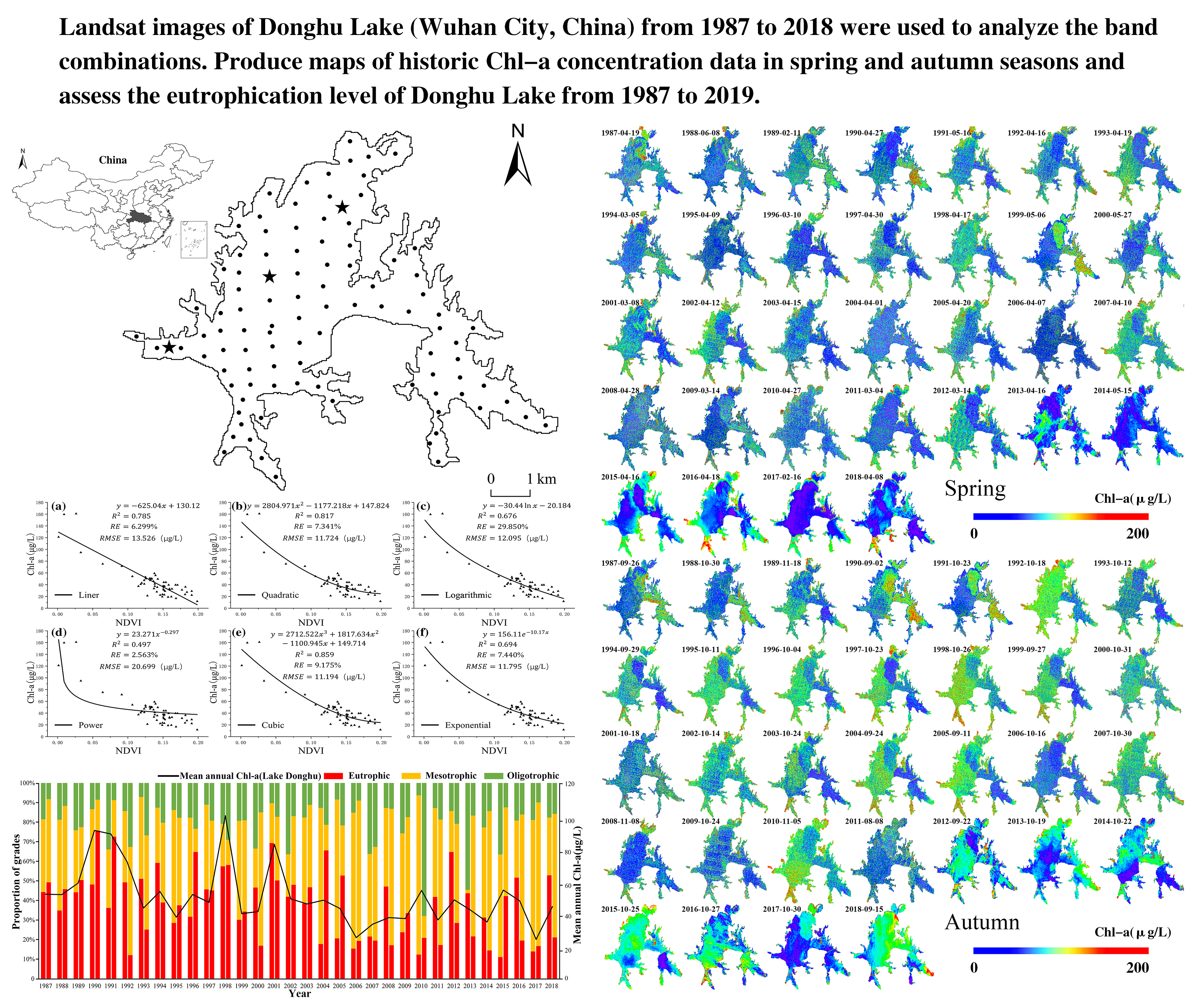
4.2. Distribution of Chl-a Concentration in Spring and Autumn from 1987 to 2018

An inversion model (Formula 6) of Chl-a concentration was applied to images of Donghu Lake captured by Landsat series satellites from 1987 to 2018. A total of 64 scenes in spring and autumn seasons were selected (Figure S2 in the Supplementary Materials). In the past 30 years, the Chl-a concentration in Donghu Lake has varied in the range of 20–200 ug/L. The higher values, even the peak ones, of Chl-a concentration were commonly found in sub-lakes such as Yujia Hu, Tuan Hu, Miao Hu and Shuiguo Hu. The Chl-a concentration in the regions between the edges of these lakes and the land was higher than that in the centers of the lakes. The water quality of Guozheng Hu and Tangling Hu was relatively good. According to the perennial analysis of Chl-a concentration, the southern part (Miao Hu, Yujia Hu) of Donghu Lake had the highest Chl-a concentration, followed by the western part (Shuiguo Hu), the eastern part (Tuan Hu, Hou Hu) and the northern part (Tangling Hu, Xiaotan Hu).
In spring, the Chl-a concentration in the eastern (Tuan Hu, Hou Hu) and southern (Yujia Hu, Miao Hu) parts of Donghu Lake was obviously higher than that in the northern (Tangling Hu, Shaoji Hu, Xiaotan Hu) and western (Shuiguo Hu, Tiane Hu) parts. In autumn, the peak values of Chl-a concentration appeared in the southern (Yujia Hu, Miao Hu, Lingjiao Hu) and eastern (Tuan Hu) parts. The area of Donghu Lake was relatively small and the meteorological conditions of each sub-lake, such as light and temperature, were similar. However, the input levels of nutrients and conditions at the bottoms of these sub-lakes were quite different. Being less affected by human activities, the western part of Donghu Lake, including Shaoji Hu and Tiane Hu, had a shallow water depth, high transparency and excellent water quality, thus providing good conditions for the growth of aquatic plants and imposing restraints on that of algae. The water flow of Guozheng Hu in the main lake region was faster. Some studies have shown that the too fast water flow and frequent water exchanges will effectively restrain the growth and aggregation of algae by damaging the growing and breeding environment of algae [22,47]. There were quite a few branches and bays of sub-lakes, such as Tuan Hu and Hou Hu in the eastern part of Donghu Lake, where culture-based fisheries have been developed [33]. In spring, the Chl-a concentration in Donghu Lake was generally low, but the pollution in it was still serious, for a large amount of sewage had been discharged into it from the dense commercial districts, residential districts and universities around Miao Hu and quite a few villages and towns around Lingjiao Hu. In autumn, the overall Chl-a concentration in Donghu Lake was relatively high and the difference of Chl-a concentration between different regions in the whole lake became smaller. The peak values of Chl-a concentration mainly appeared in relatively closed sub-lakes such as Yujia Hu, Miao Hu, Tuan Hu and Lingjiao Hu.

4.3. Trophic State Assessment

According to the results of an investigation in Donghu Lake on 18 April 2016, the TLI (Chl-a), TLI (TP), TLI (TN), TLI (SD), TLI (COD) and TLI (∑) were 64.38, 58.49, 58.68, 56.35, 79.15 and 63.49, respectively. The water quality of Donghu Lake was moderate eutrophication. The higher comprehensive TLI appeared in sub-lakes such as Miao Hu (TLI (∑) = 74.5), Shuiguo Hu (TLI (∑) = 80), Tuan Hu (TLI (∑) = 66.7), Yujia Hu (TLI (∑) = 69.6) and Hou Hu (TLI (∑) = 66.2), and the lower ones occurred in Guozheng Hu (TLI (∑) = 60.3) and Tangling Hu (TLI (∑) = 60.8). All of these were consistent with the results of remote sensing inversion of Chl-a concentration.
The comprehensive trophic level index was calculated and graduation statistics were carried out with remote sensing inversion results of Chl-a values of spring and autumn seasons from 1987 to 2018 (Figure 7). The TLI of Donghu Lake varied substantially in different periods and it was mostly mesotrophic and eutrophic. More than 70% of the total lake area was in the status of mesotrophication or eutrophication. The results indicated that the water pollution in Donghu Lake has been relatively serious during its history.
Connected with the Yangtze River, Donghu Lake used to be an open water lake with intense water exchanges and good water quality and its water levels depended on the fluctuation of the Yangtze River, according to historical data. In the 1950s, Wuhan’s municipal government made great efforts to develop iron and steel enterprises. The construction of the Wufeng Sluice and the Qingshan Central Pump during that time led to the complete separation of Donghu Lake and the Yangtze River and transformed Donghu Lake from a natural lake into an inland water body. Donghu Lake was in the stage of transition from a mesotrophic lake to a eutrophic one. In the 1960s, hundreds of factories and enterprises were built around the lake and the surrounding population increased rapidly, which caused an increase in sewage discharge. At the same time, a large number of dams and bridges were built and fisheries were vigorously developed, which led to the separation of the branches of Donghu Lake and a weakened water mobility. The surface flow velocity was only 5–10 cm/s and water at the bottom layer was basically stagnant. Human-induced eutrophication became increasingly prominent in the 1970s when Sha Hu was connected to Donghu Lake for city drainage. A large amount of organic matters, inorganic fertilizers, pesticides, poisonous substances and heavy metals such as cadmium (Cd) and manganese (Mn) were discharged into this lake. The peak volume of the sewage discharged into it exceeded 3 × 10⁵ t/d per day. The transparency of the water body and the coverage of aquatic plants decreased and the biodiversity and resource storage drastically declined. The water in Donghu Lake became muddy and smelly and the ecological balance was destroyed. Donghu Lake at that time became extremely eutrophic. In the 1980s, the number of plankton boomed in the branching streams. In 1985, serious cyanobacterial blooms broke out across the whole lake. In the 1990s, Wuhan’s government began to treat urban sewage by adopting various engineering measures such as external sewage interception, internal sewage removal, ecological restoration and water level regulation [30], which improved the water quality of Donghu Lake in the years that followed in spite of its instability. At the beginning of the 20th century, some sewage interception and decontamination projects were put into use, and the large sewage draining exits in Miao Hu, the southern part of Donghu Lake, and the Hongshan District were closed. With these measures, the water quality of Donghu Lake was tremendously improved. However, it was still in the status of eutrophication.

5. Conclusions

Taking Donghu Lake as the research object, this study built a model between Chl-a values and the band combination of (B4 − B3)/(B4 + B3) based on the remote sensing band characteristics of Chl-a, by establishing correspondence between the water quality parameters of Chl-a, TN, TP, COD and SD collected from 97 locations on 18 April 2016 and remote sensing images captured by Landsat satellites on the same day. The model was applied to images from 1987 to 2018 to obtain the long-term dynamics of Chl-a concentration in Donghu Lake. Through analysis, conclusions were reached as follows:
(1)
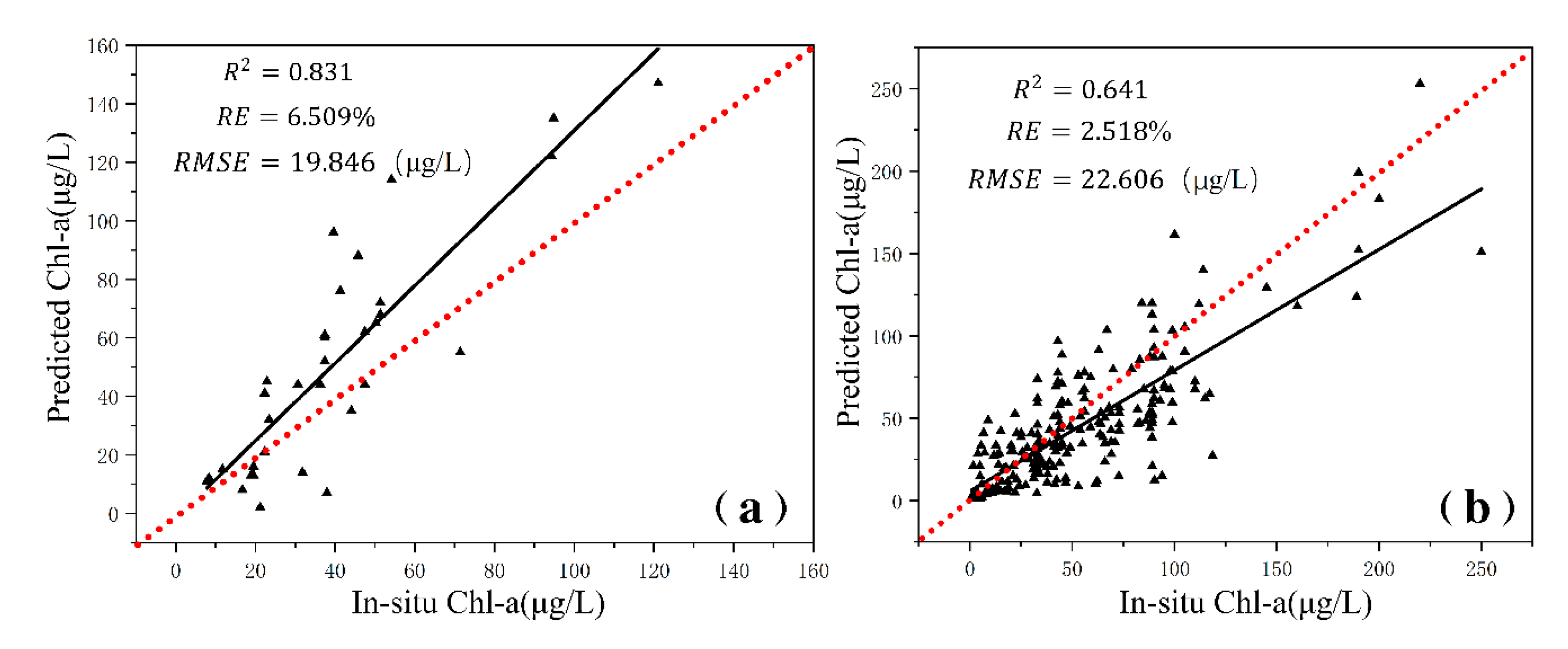
An inversion model of Chl-a concentration was established with remote sensing images and water quality parameter data. The correlation coefficient (R2) of the model was 0.859, the root mean square error (RMSE) was 11.194 μg/L and the relative error (RE) was 9.175%. The R2, RE and RMSE of the verification model were 0.831, 6.509% and 19.846 μg/L respectively. The generated results were reliable for the inversion of Chl-a concentration.
(2)
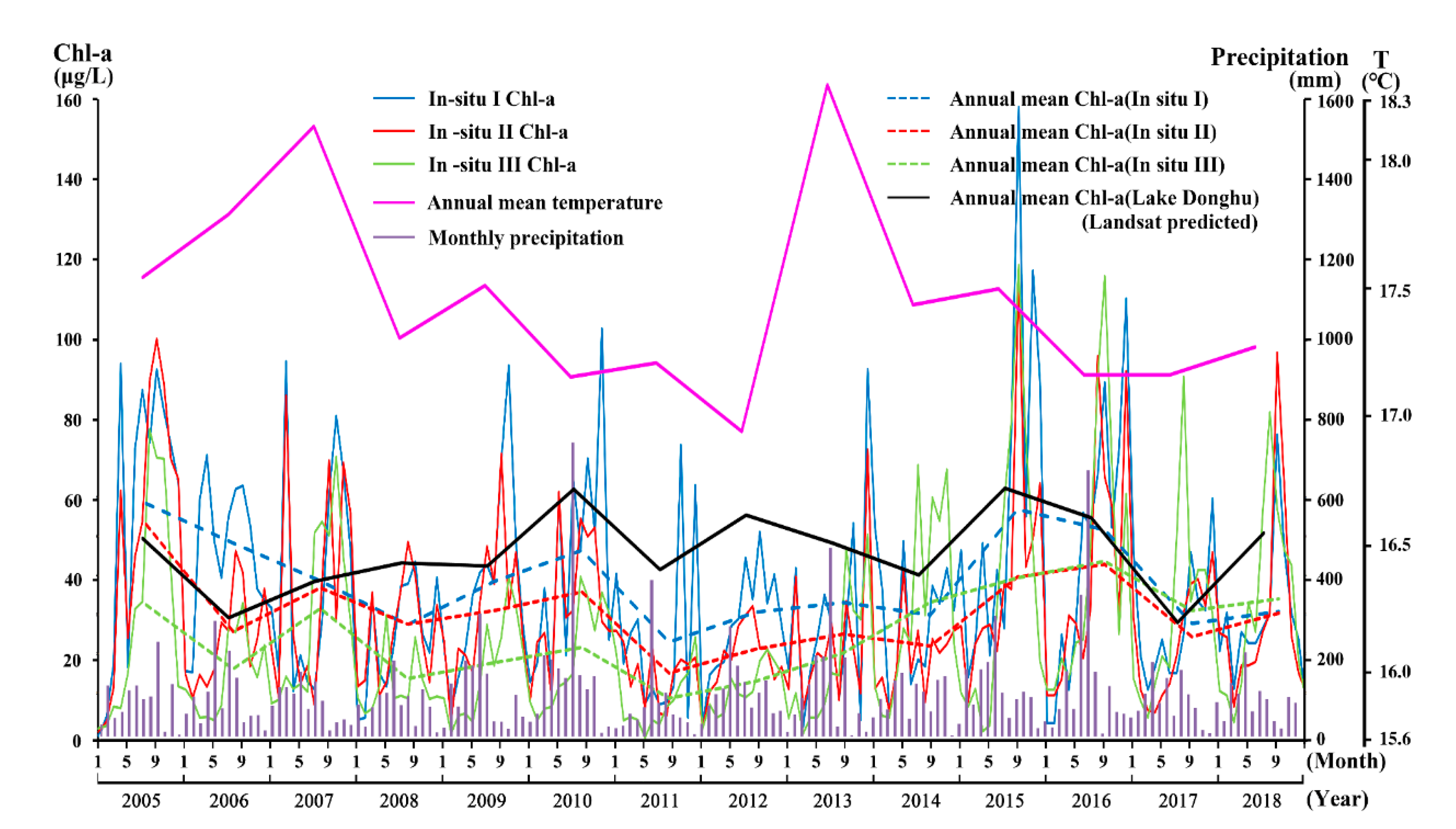
Based on the measured data and meteorological data from 2005 to 2018 in Donghu Lake, it was shown that Chl-a concentration in this lake varied in different seasons and was affected by lake morphology and distribution of surrounding pollution sources, exhibiting obvious spatio-temporal characteristics. The interannual variance analysis indicated that the Chl-a concentration in Donghu Lake was relatively high in warmer years or rainy years, and the seasonal variance analysis showed that Donghu Lake had the highest Chl-a concentration in summer, followed successively by autumn, spring and winter. The pollution levels of water in the sub-lakes were higher than those in the main lake area. Among these sub-lakes, Yujia Hu, Miao Hu and Shuiguo Hu were the three most polluted regions. The comprehensive trophic level index TLI (∑) of Donghu Lake in April 2016 was 63.49, indicating eutrophication at that time.
(3)
The accuracy of the model was verified using the data collected over more than ten years in three long-term monitoring points, which were provided by the Donghu Experimental Station of Lake Ecosystems, Chinese Academy of Sciences. The R2, RE and RMSE were 0.641, 2.518% and 22.606 μg/L, respectively. The accuracy is sufficient for conducting a remote sensing inversion, which demonstrates that the Landsat series data can be used for retrieving the long-term Chl-a concentration in inland lakes.
(4)
Historically, Donghu Lake was connected with the Yangtze River. The sub-lakes of Donghu Lake had high fluidity, good water quality and abundant aquatic plants. However, urbanization and human intervention have exerted enormous impacts on Donghu Lake. The lake’s biodiversity has been destroyed and its water quality has declined sharply. The situation has been somewhat improved through a variety of engineering measures and ecological management, showing that the building of the eco-water network of Donghu Lake has been effective for the restoration of its ecological structure and the improvement of its water quality.

Supplementary Materials

The following are available online at https://www.mdpi.com/2073-4441/12/8/2192/s1, Figure S1. Comparison between the observed and predicted Chl-a and meteorological data from 2005–2018. Figure S2: Map of predicted Chl-a concentration distribution in the spring and autumn from 1987 to 2018.

Author Contributions

Conceptualization, X.Y. and X.D.; methodology, X.Y. and X.D.; software, X.Y. and Z.Y.; investigation, X.D.; data curation, X.D.; writing—original draft preparation, X.Y., X.D. and Y.Z.; writing—review and editing, Y.J.; supervision, Y.J.; funding acquisition, Y.J. and X.D. All authors have read and agreed to the published version of the manuscript.

Funding

This research was funded by the Strategic Priority Research Program of Chinese Academy of Sciences (grant no. XDA19020301), the Fundamental Research Funds for the Central Universities (grant no. CCNU19TS001) and the National Natural Science Foundation of China (grant no. 31700400).

Acknowledgments

We thank Wenxia Tan and Chunmian Yang for inspiration and guidance of the article. We also appreciate the insightful and constructive comments and suggestions from the anonymous reviewers and the Editor that helped improve the quality of the manuscript.

Conflicts of Interest

The authors declare no conflict of interest. The funders had no role in the design of the study; in the collection, analyses, or interpretation of data; in the writing of the manuscript, or in the decision to publish the results.

References

  1. Chen, Q.; Huang, M.; Tang, X. Eutrophication assessment of seasonal urban lakes in China Yangtze River Basin using Landsat 8-derived Forel-Ule index: A six-year (2013–2018) observation. Sci. Total Environ. 2019. [Google Scholar] [CrossRef] [PubMed]
  2. Xie, C.; Huang, X.; Wang, L.; Fang, X.; Liao, W. Spatiotemporal change patterns of urban lakes in China’s major cities between 1990 and 2015. Int. J. Digit. Earth 2017, 11, 1085–1102. [Google Scholar] [CrossRef]
  3. Hamer, A.J.; Parris, K.M. Local and landscape determinants of amphibian communities in urban ponds. Ecol. Appl. 2011, 21, 378–390. [Google Scholar] [CrossRef] [PubMed]
  4. Deutsch, E.S.; Alameddine, I.; El-Fadel, M. Monitoring water quality in a hypereutrophic reservoir using Landsat ETM+ and OLI sensors: How transferable are the water quality algorithms? Environ. Monit. Assess 2018, 190, 141. [Google Scholar] [CrossRef]
  5. Yang, H.; Yi, C.; Xie, P.; Xing, Y.; Ni, L. Sedimentation rates, nitrogen and phosphorus retentions in the largest urban Lake Donghu, China. J. Radioanal. Nucl. Chem. 2005, 267, 205–208. [Google Scholar] [CrossRef] [Green Version]
  6. Durovic, B.; Durovic, I.; Joksimovic, A.; Crnojevic, V.; Dukanovic, S.; Pestoric, B. Monitoring the eutrophication using Landsat 8 in the Boka Kotorska Bay. Acta Adriat. 2018, 59, 17–33. [Google Scholar] [CrossRef] [Green Version]
  7. Song, K.; Liu, G.; Wang, Q.; Wen, Z.; Lyu, L.; Du, Y.; Sha, L.; Fang, C. Quantification of lake clarity in China using Landsat OLI imagery data. Remote Sens. Environ. 2020, 243. [Google Scholar] [CrossRef]
  8. Tang, H.; Xie, P.; Hong, L. Changes in the Phytoplankton Community of Lake Donghu Since the 1980s. J. Freshwater Ecol. 2005, 20, 591–594. [Google Scholar] [CrossRef] [Green Version]
  9. Han, X.; Feng, L.; Chen, X.; Yesou, H. MERIS observations of chlorophyll-a dynamics in Erhai Lake between 2003 and 2009. Int. J. Remote Sens. 2014, 35, 8309–8322. [Google Scholar] [CrossRef]
  10. Guo, Q.; Wu, X.; Bing, Q.; Pan, Y.; Wang, Z.; Fu, Y.; Wang, D.; Liu, J. Study on Retrieval of Chlorophyll-a Concentration Based on Landsat OLI Imagery in the Haihe River, China. Sustainability 2016, 8, 758. [Google Scholar] [CrossRef] [Green Version]
  11. Bocharov, A.V.; Tikhomirov, O.A.; Khizhnyak, S.D.; Pakhomov, P.M. Monitoring of Chlorophyll in Water Reservoirs Using Satellite Data. J. Appl. Spectrosc. 2017, 84, 291–295. [Google Scholar] [CrossRef]
  12. Yip, H.D.; Johansson, J.; Hudson, J.J. A 29-year assessment of the water clarity and chlorophyll-a concentration of a large reservoir: Investigating spatial and temporal changes using Landsat imagery. J. Great Lakes Res. 2015, 41, 34–44. [Google Scholar] [CrossRef]
  13. Fu, Y.; Xu, S.; Zhang, C.; Sun, Y. Spatial downscaling of MODIS Chlorophyll-a using Landsat 8 images for complex coastal water monitoring. Estuari. Coast. Shelf Sci. 2018, 209, 149–159. [Google Scholar] [CrossRef]
  14. Markogianni, V.; Kalivas, D.; Petropoulos, G.; Dimitriou, E. An Appraisal of the Potential of Landsat 8 in Estimating Chlorophyll-a, Ammonium Concentrations and Other Water Quality Indicators. Remote Sens. 2018, 10, 1018. [Google Scholar] [CrossRef] [Green Version]
  15. Poddar, S.; Chacko, N.; Swain, D. Estimation of Chlorophyll-a in Northern Coastal Bay of Bengal Using Landsat-8 OLI and Sentinel-2 MSI Sensors. Front. Mar. Sci. 2019, 6. [Google Scholar] [CrossRef]
  16. Allan, M.G.; Hamilton, D.P.; Hicks, B.; Brabyn, L. Empirical and semi-analytical chlorophyll a algorithms for multi-temporal monitoring of New Zealand lakes using Landsat. Environ. Monit. Assess 2015, 187, 364. [Google Scholar] [CrossRef]
  17. Gilerson, A.A.; Gitelson, A.A.; Zhou, J.; Gurlin, D.; Moses, W.; Ioannou, I.; Ahmed, S.A. Algorithms for remote estimation of chlorophyll-a in coastal and inland waters using red and near infrared bands. Opt. Express 2010, 18, 24109–24125. [Google Scholar] [CrossRef] [Green Version]
  18. Gitelson, A.A.; Schalles, J.F.; Hladik, C.M. Remote chlorophyll-a retrieval in turbid, productive estuaries: Chesapeake Bay case study. Remote Sens. Environ. 2007, 109, 464–472. [Google Scholar] [CrossRef]
  19. Yacobi, Y.Z.; Moses, W.J.; Kaganovsky, S.; Sulimani, B.; Leavitt, B.C.; Gitelson, A.A. NIR-red reflectance-based algorithms for chlorophyll-a estimation in mesotrophic inland and coastal waters: Lake Kinneret case study. Water Res. 2011, 45, 2428–2436. [Google Scholar] [CrossRef] [Green Version]
  20. Jiang, G.; Loiselle, S.A.; Yang, D.; Ma, R.; Su, W.; Gao, C. Remote estimation of chlorophyll a concentrations over a wide range of optical conditions based on water classification from VIIRS observations. Remote Sens. Environ. 2020, 241. [Google Scholar] [CrossRef]
  21. Xu, J.; Gao, C.; Wang, Y. Extraction of Spatial and Temporal Patterns of Concentrations of Chlorophyll-a and Total Suspended Matter in Poyang Lake Using GF-1 Satellite Data. Remote Sens. 2020, 12, 622. [Google Scholar] [CrossRef] [Green Version]
  22. Feng, L.; Hu, C.; Han, X.; Chen, X.; Qi, L. Long-Term Distribution Patterns of Chlorophyll-a Concentration in China’s Largest Freshwater Lake: MERIS Full-Resolution Observations with a Practical Approach. Remote Sens. 2014, 7, 275–299. [Google Scholar] [CrossRef] [Green Version]
  23. Yang, W.; Matsushita, B.; Chen, J.; Fukushima, T.; Ma, R. An Enhanced Three-Band Index for Estimating Chlorophyll-a in Turbid Case-II Waters: Case Studies of Lake Kasumigaura, Japan, and Lake Dianchi, China. IEEE Geosci. Remote Sens. Lett. 2010, 7, 655–659. [Google Scholar] [CrossRef] [Green Version]
  24. Tan, W.; Liu, P.; Liu, Y.; Yang, S.; Feng, S. A 30-Year Assessment of Phytoplankton Blooms in Erhai Lake Using Landsat Imagery: 1987 to 2016. Remote Sens. 2017, 9, 1265. [Google Scholar] [CrossRef] [Green Version]
  25. Li, J.; Zhang, Y.; Ma, R.; Duan, H.; Loiselle, S.; Xue, K.; Liang, Q. Satellite-Based Estimation of Column-Integrated Algal Biomass in Nonalgae Bloom Conditions: A Case Study of Lake Chaohu, China. IEEE J. Sel. Top. Appl. Earth Obs. Remote Sens. 2017, 10, 450–462. [Google Scholar] [CrossRef]
  26. Liu, X.; Qian, K.; Chen, Y.; Gao, J. A comparison of factors influencing the summer phytoplankton biomass in China’s three largest freshwater lakes: Poyang, Dongting, and Taihu. Hydrobiologia 2016, 792, 283–302. [Google Scholar] [CrossRef]
  27. Zhang, Y.; He, F.; Kong, L.; Liu, B.; Zhou, Q.; Wu, Z. Release characteristics of sediment P in all fractions of Donghu Lake, Wuhan, China. Desalin. Water Treat. 2016, 57, 25572–25580. [Google Scholar] [CrossRef]
  28. Ji, L.; Berezina, N.A.; Golubkov, S.M.; Cao, X.; Golubkov, M.S.; Song, C.; Umnova, L.P.; Zhou, Y. Phosphorus flux by macrobenthic invertebrates in a shallow eutrophic lake Donghu: Spatial change. Know. Manag. Aquat. Ecosyst. 2011. [Google Scholar] [CrossRef] [Green Version]
  29. Chen, X.; Li, H.; Hou, J.; Cao, X.; Song, C.; Zhou, Y. Sediment–water interaction in phosphorus cycling as affected by trophic states in a Chinese shallow lake (Lake Donghu). Hydrobiologia 2016, 776, 19–33. [Google Scholar] [CrossRef]
  30. Jiao, Y.; Xu, L.; Li, Q.; Gu, S. Thin-layer fine-sand capping of polluted sediments decreases nutrients in overlying water of Wuhan Donghu Lake in China. Environ. Sci. Pollut. Res. Int. 2020, 27, 7156–7165. [Google Scholar] [CrossRef]
  31. Yan, Q.; Stegen, J.C.; Yu, Y.; Deng, Y.; Li, X.; Wu, S.; Dai, L.; Zhang, X.; Li, J.; Wang, C.; et al. Nearly a decade-long repeatable seasonal diversity patterns of bacterioplankton communities in the eutrophic Lake Donghu (Wuhan, China). Mol. Ecol. 2017, 26, 3839–3850. [Google Scholar] [CrossRef] [PubMed]
  32. Zhang, X.; Yan, Q.; Yu, Y.; Dai, L. Spatiotemporal pattern of bacterioplankton in Donghu Lake. Chin. J. Oceanol. Limnol. 2014, 32, 554–564. [Google Scholar] [CrossRef]
  33. Tang, H.; Xie, P. Budgets and Dynamics of Nitrogen and Phosphorus in a Shallow, Hypereutrophic Lake in China. J. Freshwater Ecol. 2000, 15, 505–514. [Google Scholar] [CrossRef]
  34. Deng, X.; Chen, J.; Hansson, L.-A.; Zhao, X.; Xie, P. Eco-chemical mechanisms govern phytoplankton emissions of dimethylsulfide in global surface waters. Natl. Sci. Rev. 2020. [Google Scholar] [CrossRef]
  35. Domínguez, E.; Aguado, S.; García, G. Monitoring Coastal Lagoon Water Quality Through Remote Sensing: The Mar Menor as a Case Study. Water 2019, 11, 1468. [Google Scholar] [CrossRef] [Green Version]
  36. Du, Y.; Song, K.; Liu, G.; Wen, Z.; Fang, C.; Shang, Y.; Zhao, F.; Wang, Q.; Du, J.; Zhang, B. Quantifying total suspended matter (TSM) in waters using Landsat images during 1984–2018 across the Songnen Plain, Northeast China. J. Environ. Manag. 2020, 262, 110334. [Google Scholar] [CrossRef]
  37. Ayeni, A.O.; Adesalu, T.A. Validating chlorophyll-a concentrations in the Lagos Lagoon using Remote Sensing extraction and laboratory fluorometric methods. MethodsX 2018, 5, 1204–1212. [Google Scholar] [CrossRef]
  38. Ha, N.T.T.; Koike, K.; Nhuan, M.T.; Canh, B.D.; Thao, N.T.P.; Parsons, M. Landsat 8/OLI Two Bands Ratio Algorithm for Chlorophyll-A Concentration Mapping in Hypertrophic Waters: An Application to West Lake in Hanoi (Vietnam). IEEE J. Sel. Top. Appl. Earth Obs. Remote Sens. 2017, 10, 4919–4929. [Google Scholar] [CrossRef]
  39. Watanabe, F.; Alcantara, E.; Rodrigues, T.; Rotta, L.; Bernardo, N.; Imai, N. Remote Sensing of the chlorophyll-a based on OLI/Landsat-8 and MSI/Sentinel-2A (Barra Bonita reservoir, Brazil). Anais da Academia Brasileira de Ciencias 2018, 90, 1987–2000. [Google Scholar] [CrossRef] [Green Version]
  40. Yang, Y.; Liu, Y.; Zhou, M.; Zhang, S.; Zhan, W.; Sun, C.; Duan, Y. Landsat 8 OLI image based terrestrial water extraction from heterogeneous backgrounds using a reflectance homogenization approach. Remote Sens. Environ. 2015, 171, 14–32. [Google Scholar] [CrossRef]
  41. Barrett, D.; Frazier, A. Automated Method for Monitoring Water Quality Using Landsat Imagery. Water 2016, 8, 257. [Google Scholar] [CrossRef] [Green Version]
  42. Murugan, P.; Sivakumar, R.; Pandiyan, R.; Annadurai, M. Comparison of in-situ Hyperspectral and Landsat ETM+ Data for Chlorophyll-a Mapping in Case-II Water (Krishnarajapuram Lake, Bangalore). J. Indian Soc. Remote Sens. 2016, 44, 949–957. [Google Scholar] [CrossRef]
  43. Moses, W.J.; Gitelson, A.A.; Perk, R.L.; Gurlin, D.; Rundquist, D.C.; Leavitt, B.C.; Barrow, T.M.; Brakhage, P. Estimation of chlorophyll-a concentration in turbid productive waters using airborne hyperspectral data. Water Res. 2012, 46, 993–1004. [Google Scholar] [CrossRef] [PubMed] [Green Version]
  44. Othman, Y.; Steele, C.; Hilaire, R.S. Surface Reflectance Climate Data Records (CDRs) is a Reliable Landsat ETM+ Source to Study Chlorophyll Content in Pecan Orchards. J. Indian Soc. Remote Sens. 2017, 46, 211–218. [Google Scholar] [CrossRef]
  45. Khattab, M.F.O.; Merkel, B.J. Application of Landsat 5 and Landsat 7 images data for water quality mapping in Mosul Dam Lake, Northern Iraq. Arab. J. Geosci. 2013, 7, 3557–3573. [Google Scholar] [CrossRef]
  46. Pardo-Pascual, J.E.; Almonacid-Caballer, J.; Ruiz, L.A.; Palomar-Vázquez, J. Automatic extraction of shorelines from Landsat TM and ETM+ multi-temporal images with subpixel precision. Remote Sens. Environ. 2012, 123, 1–11. [Google Scholar] [CrossRef] [Green Version]
  47. Yao, J.; Wang, G.; Xue, B.; Wang, P.; Hao, F.; Xie, G.; Peng, Y. Assessment of lake eutrophication using a novel multidimensional similarity cloud model. J. Environ. Manag. 2019, 248, 109259. [Google Scholar] [CrossRef]
  48. Roy, D.P.; Wulder, M.A.; Loveland, T.R.; Woodcock, C.E.; Allen, R.G.; Anderson, M.C.; Helder, D.; Irons, J.R.; Johnson, D.M.; Kennedy, R.; et al. Landsat-8: Science and product vision for terrestrial global change research. Remote Sens. Environ. 2014, 145, 154–172. [Google Scholar] [CrossRef] [Green Version]
  49. Yu, G.; Yang, W.; Matsushita, B.; Li, R.; Oyama, Y.; Fukushima, T. Remote Estimation of Chlorophyll-a in Inland Waters by a NIR-Red-Based Algorithm: Validation in Asian Lakes. Remote Sens. 2014, 6, 3492–3510. [Google Scholar] [CrossRef] [Green Version]
  50. Manzar Abbas, M.; Melesse, A.M.; Scinto, L.J.; Rehage, J.S. Satellite Estimation of Chlorophyll-a Using Moderate Resolution Imaging Spectroradiometer (MODIS) Sensor in Shallow Coastal Water Bodies: Validation and Improvement. Water 2019, 11, 1621. [Google Scholar] [CrossRef] [Green Version]
  51. Duan, H.; Ma, R.; Xu, X.; Kong, F.; Zhang, S.; Kong, W.; Hao, J.; Shang, L. Two-decade reconstruction of algal blooms in China’s Lake Taihu. Environ. Sci. Technol. 2009, 43, 3522–3528. [Google Scholar] [CrossRef] [PubMed]
  52. Torbick, N.; Hu, F.; Zhang, J.Y.; Qi, J.G.; Zhang, H.J.; Becker, B. Mapping Chlorophyll-a Concentrations in West Lake, China using Landsat 7 ETM+. J. Great Lakes Res. 2008, 34, 559–565. [Google Scholar] [CrossRef]
  53. Liu, X.; Wu, Q.; Chen, Y.; Dokulil, M.T. Imbalance of plankton community metabolism in eutrophic Lake Taihu, China. J. Great Lakes Res. 2011, 37, 650–655. [Google Scholar] [CrossRef]
  54. Zhang, Y.; Ma, R.; Zhang, M.; Duan, H.; Loiselle, S.; Xu, J. Fourteen-Year Record (2000–2013) of the Spatial and Temporal Dynamics of Floating Algae Blooms in Lake Chaohu, Observed from Time Series of MODIS Images. Remote Sens. 2015, 7, 10523–10542. [Google Scholar] [CrossRef] [Green Version]
  55. Bonansea, M.; Rodriguez, M.C.; Pinotti, L.; Ferrero, S. Using multi-temporal Landsat imagery and linear mixed models for assessing water quality parameters in Río Tercero reservoir (Argentina). Remote Sens. Environ. 2015, 158, 28–41. [Google Scholar] [CrossRef]
Figure 1. Study area and in situ chlorophyll-a (Chl-a) sampling locations.
Water 12 02192 g001
Figure 2. (a) Water spectral curves before and after FLAASH Atmospheric Correction. (b) A true-color composite Landsat-8 OLI image acquired on 18 April 2016 after an extraction of the water body information.
Water 12 02192 g002
Figure 3. Comparison between in situ Chl-a and (B4 − B3)/(B4 + B3) using different algorithms, including (a) linear; (b) quadratic; (c) logarithmic; (d) power; (e) cubic and (f) exponential.
Water 12 02192 g003
Figure 4. (a) Landsat-predicted versus actual Chl-a concentration. (b) Landsat-predicted versus actual Chl-a concentration (three long-term monitoring points from 2005 to 2018). The 1:1 line is represented by the red dashed line and the black solid line represents the observed correlation between the Landsat estimated values and actual measured values.
Water 12 02192 g004
Figure 5. Comparison of the observed (a) and Landsat-predicted (b) Chl-a concentration distribution map on 18 April 2016.
Water 12 02192 g005
Figure 6. Comparison between the observed and predicted Chl-a and meteorological data from 2005–2018.
Water 12 02192 g006
Figure 7. The area ratio of different Chl-a concentration grades from 1987 to 2018. The black solid line represents the annual mean value of Chl-a. The column on the left represents the proportion of grades in spring of different years and the column on the right represents that in autumn.
Water 12 02192 g007
Table 1. Landsat image acquisition date and sensor type.
Landsat DateSensorLandsat DateSensorLandsat DateSensor
19April 1987Landsat-5/TM23 October 1997Landsat-5/TM28 April 2008Landsat-5/TM
26 September 1987Landsat-5/TM17 April 1998Landsat-5/TM8 November 2008Landsat-5/TM
8 June 1988Landsat-5/TM26 October 1998Landsat-5/TM14 March 2009Landsat-5/TM
30 October 1988Landsat-5/TM6 May 1999Landsat-5/TM24 October 2009Landsat-5/TM
11 February 1989Landsat-5/TM27 September 1999Landsat-5/TM27 April 2010Landsat-5/TM
18 November 1989Landsat-5/TM27 May 2000Landsat-5/TM5 November 2010Landsat-5/TM
27 April 1990Landsat-5/TM31 October 2000Landsat-5/TM4 March 2011Landsat-5/TM
2 September 1990Landsat-5/TM8 March 2001Landsat-5/TM8 August 2011Landsat-5/TM
16 May 1991Landsat-5/TM18 October 2001Landsat-5/TM14 March 2012Landsat-7/ETM+
23 October 1991Landsat-5/TM12 April 2002Landsat-5/TM16 April 2013Landsat-8 OLI
16 April 1992Landsat-5/TM14 October 2002Landsat-5/TM19 October 2013Landsat-8 OLI
18 October 1992Landsat-5/TM15 April 2003Landsat-5/TM15 May 2014Landsat-8 OLI
19 April 1993Landsat-5/TM24 October 2003Landsat-5/TM22 October 2014Landsat-8 OLI
12 October 1993Landsat-5/TM1 April 2004Landsat-5/TM16 April 2015Landsat-8 OLI
5 March 1994Landsat-5/TM24 September 2004Landsat-5/TM25 October 2015Landsat-8 OLI
29 September 1994Landsat-5/TM20 April 2005Landsat-5/TM18 April 2016Landsat-8 OLI
9 April 1995Landsat-5/TM11 September 2005Landsat-5/TM27 October 2016Landsat-8 OLI
11 October 1995Landsat-5/TM07 April 2006Landsat-5/TM16 February 2017Landsat-8 OLI
10 March 1996Landsat-5/TM16 October 2006Landsat-5/TM30 October 2017Landsat-8 OLI
4 October 1996Landsat-5/TM10 April 2007Landsat-5/TM8 April 2018Landsat-8 OLI
30 April 1997Landsat-5/TM30 October 2007Landsat-5/TM15 September 2018Landsat-8 OLI
Table 2. Correlation coefficients rij and r i j 2 between some parameters and Chl-a of lakes (reservoirs) in China.
ParameterChl-aTPTNSDCODMn
rij10.840.82−0.830.83
r i j 2
10.70560.67240.68890.6889
Note: This table is cited from China’s Lake Environment. The correlation coefficient rij in this table was derived from the results of survey data of 26 major lakes in China.
Table 3. Band specifications for Landsat sensors. The bands used in this study are shown in bold.
Spectral ChannelLandsat-8 OLILandsat-7/ETM+Landsat-5/TM
BandsWavelength (μm)BandsWavelength (μm)BandsWavelength (μm)
Band 1Coastal0.43–0.45Blue0.45–0.52Blue0.45–0.52
Band 2Blue0.45–0.51Green0.52–0.60Green0.52–0.60
Band 3Green0.53–0.59Red0.63–0.69Red0.63–0.69
Band 4Red0.64–0.67Near-Infrared0.77–0.90Near-Infrared0.76–0.90
Band 5Near-Infrared0.85–0.88Near-Infrared1.55–1.75Near-Infrared1.55–1.75
Band 6SWIR 11.57–1.65Thermal10.40–12.50Thermal10.40–12.50
Band 7SWIR 22.11–2.29Mid-Infrared2.08–2.35Mid-Infrared2.08–2.35
Band 8Panchromatic0.50–0.68Panchromatic0.52–0.90
Band 9Cirrus1.36–1.38
Band 10TIRS 110.60–11.19
Band 11TIRS 211.50–12.51
Table 4. Correlation coefficient of Landsat-8 OLI band combinations with Chl-a concentration.
BandrpBandrpBandrp
B1−0.458 **0.0000B3/B2−0.288 *0.0111B3/(B1 + B4)−0.607 **0.0000
B2−0.458 **0.0000B3/B4−0.609 **0.0000B3/(B2 + B4)−0.532 **0.0000
B3−0.500 **0.0000B4/B1−0.265 *0.0197B3/(B1 + B2 + B4)−0.582 **0.0000
B4−0.414 **0.0002B4/B20.400 **0.0003B4/(B1 + B2)−0.0650.5755
B5−0.1660.1494B4/B30.605 **0.0000B4/(B1 + B3)0.2140.0615
B6−0.0870.4542B1/(B2 + B3)0.526 **0.0000B4/(B2 + B3)0.606 **0.0000
B7−0.0620.5941B1/(B2 + B4)0.391 **0.0004B4/(B1 + B2 + B3)0.313 **0.0056
B1/B20.444 **0.0001B1/(B3 + B4)0.475 **0.0000(B1 − B2)/(B1 + B2)0.462 **0.0000
B1/B30.546 **0.0000B1/(B2 + B3 + B4)0.479 **0.0000(B1 − B3)/(B1 + B3)−0.263 *0.0210
B1/B40.284 *0.0122B2/(B1 + B3)−0.240 *0.0352(B1 − B4)/(B1 + B4)0.268 *0.0183
B2/B10.465 **0.0000B2/(B1 + B4)−0.500 **0.0000(B2 − B3)/(B2 + B3)−0.321 **0.0044
B2/B30.342 **0.0023B2/(B3 + B4)0.0030.9770(B2 − B4)/(B2 + B4)0.401 **0.0003
B2/B4−0.399 **0.0003B2/(B1 + B3 + B4)−0.312 **0.0057(B3 − B4)/(B3 + B4)−0.826 **0.0000
B3/B1−0.534 **0.0000B3/(B1 + B2)−0.523 **0.0000(B4 − B3)/(B4 + B3)−0.826 **0.0000
* p < 0.05, ** p < 0.01.

