Article

Differences in the Vertical Distribution of Two Cladoceran Species in the Nakdong River Estuary, South Korea

National Institute of Ecology, Seo-Cheon Gun, Chungcheongnam Province 325-813, Korea
*
Author to whom correspondence should be addressed.
Water 2020, 12(8), 2154; https://doi.org/10.3390/w12082154
Submission received: 30 June 2020 / Revised: 27 July 2020 / Accepted: 28 July 2020 / Published: 30 July 2020
(This article belongs to the Section Biodiversity and Functionality of Aquatic Ecosystems)

Abstract

:
As cladocerans are a primary food source for fish, predator avoidance is important to sustain cladoceran populations. We hypothesized that Bosmina longirostris and Daphnia obtusa would show different vertical distributions that depend on environmental variables and their life cycle phase. Quarterly monitoring was implemented in three water column layers (upper, middle, and bottom) in the Nakdong River Estuary. Cladocerans were mostly observed during summer; B. longirostris and D. obtusa were most abundant and exhibited different vertical distributions. Large (>600 μm) D. obtusa individuals were mainly distributed in the bottom layer (9–11 m) during the daytime and in the upper layer (1–3 m) at night. Utilization of the bottom layer by large D. obtusa was possibly a defense strategy to avoid fish predation. Although the bottom layer was not supported by lower water temperatures and dissolved oxygen than the upper or middle layers, as suggested in the previous study, we assumed that high turbidity replaced this role as a place shunned by fish (and thus a refuge for Daphnia obtusa). In contrast, smaller individuals remained in the upper layer at all times because of the low predation risk. The consumption of B. longirostris by fish was low, as the largest B. longirostris (411 μm) was smaller than the small-sized Daphnia. From this finding, we suggest that the vertical distribution of cladocerans likely depends on selectivity feeding based on fish size rather than the presence/absence of fish. We considered that these results are an important advance in understanding distribution patterns of cladocerans related to environmental features, as well as their key predators.

1. Introduction

Predator–prey interactions are important factors that control animal behavior and ecosystem community structures [1]. Clear empirical evidence shows that predator foraging behavior is influenced by prey density gradients. In addition, predators are major sources of mortality in biological communities and play an important role in natural selection. Predators select their prey in predator–prey relationships, and under conditions of prey absence, predators may switch prey items. This predatory switching behavior requires prey species to possess various defense strategies to increase their chances of survival [1].
Prey defense strategies vary and depend on morphology [2], behavior [3], and life cycle phase [4], and may change according to environmental characteristics and the predator types present in the community. The foraging activities of fish, the representative predator of the aquatic ecosystem, also vary depending on species, which requires prey to utilize various defense strategies against the existence of diverse predators [5,6]. Prey defense strategies may be important for maintaining adequate prey–predator interactions by enhancing prey viability and predator food resource availability. Furthermore, community biodiversity depends on the proper maintenance of these predator–prey interactions, which are also measures of ecosystem health [7].
Among freshwater organisms, cladoceran predation defense strategies have evolved efficiently. Cladocerans behave like primary consumers in freshwater ecosystems and are consumed as food items by various predators, such as invertebrates and juvenile fish [8]. Cladoceran defense strategies are diverse and include behavioral changes, morphological defenses expressed during repeat molting events that last for a few days, and life cycle changes that occur over a few weeks [9]. Previous studies of Cladoceran defense behavior have mainly focused on Daphnia spp. (Daphnia galeata, Daphnia pulex, Daphnia magna) [10,11,12]. Daphnia spp. show poor swimming ability and move frequently within feeding habitats and are thus easily exposed to predators. Daphnia spp. make use of various defense strategies to avoid predation and efficiently increase their populations. Daphnia spp. in deep lakes and reservoirs show diel vertical migration (DVM), moving toward deeper water layers near the thermocline to avoid visual fish predators during the day and toward the upper layers to feed on phytoplankton at night [13,14,15]. This migration pattern occurs because predators and food sources are both found in the upper water layers. When light penetration is low within the water column, dissolved oxygen (DO) concentrations and water temperatures tend to be lower in the bottom water layers, making these habitats unsuitable for fish foraging activity but effective refuge areas for Daphnia spp. to avoid fish predation [16,17,18,19,20,21]. This Daphnia behavioral response is a survival strategy that was acquired as a result of coexistence with predators over extended periods. However, the vertical distribution may disappear when predators or food sources are absent in the upper layers [22]. The DVM pattern is closely related to fish kairomones [23]. If no such chemical cue is present, the Daphnia spp. usually stays in the upper layer continuously. Therefore, the DVM pattern in the presence of fish kairomones represents the result of a non-lethal interaction between predator (i.e., fish) and prey (i.e., Daphnia spp). Most of these behavioral defenses are related to fish predation and tend to vary when other predators, such as invertebrates, are present in high densities.
Empirical studies suggest that the vertical distribution of cladoceran communities occurs mainly in deeper lakes or reservoirs [24,25]. This is because, for the hypolimnion to be used as a refuge for cladocerans to avoid fish predation, the hypolimnion must possess unsuitable environmental conditions for the distribution of fish. Low dissolved oxygen levels or water temperatures in the hypolimnion are well-known environmental factors that induce the vertical distribution of cladocerans [26]. The vertical differences in these environmental variables are mainly a result of summer stratification. However, in previous studies, environmental variables other than dissolved oxygen or water temperature have been somewhat insufficiently studied as inducement factors for the vertical distribution of cladocerans. We theorized that if there were clear differences in other environmental variables between water layers, the different vertical distribution of cladocerans could occur even in shallow lakes and reservoirs.
In this study, we sought to elucidate the responses of two cladoceran species (Bosmina longirostris and Daphnia obtusa) to fish predation to advance our understanding of the distribution of cladoceran communities in aquatic ecosystems. Although the vertical distribution of cladocerans is strongly influenced by fish predation, all cladoceran species or individuals will not react simply to the presence or absence of fish. The two cladoceran species studied undertake cost-intensive migrations (i.e., avoids predators in time and space) to avoid being eaten. This study aimed to elucidate (1) spatial changes in cladoceran communities in relation to environmental variations (e.g., water temperature, dissolved oxygen, and turbidity), (2) the vertical distribution in relation to the body length of the two cladoceran species, and (3) the responses of cladoceran species in relation to fish predators. We hypothesized that the target species, B. longirostris and D. obtusa, would show different vertical distributions based on environmental variables and that these distributions would vary depending on their life cycle phase (i.e., body size). To test this hypothesis, we evaluated (1) the influence of turbidity conditions and water depths on the vertical distribution of B. longirostris and D. obtusa, (2) the vertical distribution of B. longirostris and D. obtusa during the daytime and at night, and (3) the consumption of the two cladoceran species (B. longirostris and D. obtusa) by dominant fish species, depending on the body length of the fish.

2. Materials and Methods

2.1. Site Description

The Nakdong River, which has an approximate drainage area of 23,817 km2, is one of the largest river systems in South Korea. In the Nakdong River, water flow is regulated by seven dams (i.e., Andong, Imha, Hapcheon, Namgang, Yeongcheon, Miryang, and Unmoon) and an estuarine barrage. This regulation results in eutrophication in the lower reaches of the river [27,28]. Furthermore, the Lower Nakdong River is impacted by several typhoons each year, resulting in major floods from June to September. The mean annual rainfall in the region is ≈1150 mm and more than 60% of the annual rainfall occurs from June to early September [29,30]. Furthermore, the annual air temperature is approximately 12.7 °C. The air and freshwater temperatures are high during the summer months [31].
The Nakdong River Estuary (NRE) was built from 1983–1987 to prevent saltwater intrusion into the estuary. The NRE is equipped with 10 gates, including four regulating gates and six main gates. All gates can be used for both underflow and overflow. The estuary barrage is 2.3 km long and includes 510 m of gate sections and a 1720 m long closed dam section. The NRE is also equipped with a navigation lock, a fish ladder, and related structures. The NRE controls the upstream water stage to prevent saltwater intrusion. As shown in Figure 1, the study area comprised three study sites located around Eulsuk Island, which is upstream from the estuary dam. The study site locations were established in the center of the reservoirs where maximum water depths were recorded.

2.2. Monitoring Strategy

The sampling of cladoceran communities and environmental data collection were conducted during four seasons (i.e., in February during winter, in May during spring, in August during summer, and in October during autumn) at each study site during the afternoon (13:00 to 16:00) of 2013 (Figure 1). To evaluate the vertical distribution of environmental variables and the zooplankton communities, we collected a total of 15 L water samples (i.e., 10 L of water for environmental variables, and 5 L of water for cladoceran collection) from each of the three water-column layers (upper, 1–3 m; middle, 4–7 m; and bottom, 7–15 m) using a 10 L Van-Dorn water sampler (Wildco Supply Company; Yulee, FL, USA). We measured the maximum water depth of each study site using an EK-500 echo sounder (SIMRAD; Lynnwood, WA, USA) to identify the three water layers of each study site.
The environmental variables (water depth, water temperature, dissolved oxygen (DO), pH, chlorophyll a, and total suspended solids (TSS)) were measured using the water samples collected from each of the study sites. A YSI Model 58 DO meter (Yellow Springs Instruments; Yellow Springs, OH, USA) was used to measure the water temperature and DO, and pH was measured using an Orion Model 250 m (Orion Research Inc.; Boston, MA, USA). The 10 L water samples were transported to the laboratory immediately after sampling to measure the concentrations of chlorophyll a and TSS. The water samples were filtered through a mixed cellulose ester (MCE, Model No. A045A047A) membrane filter with a pore size of 0.45 μm (Advantech Co.; Hyogo, Japan). The filtrates were used to determine the concentration of chlorophyll a based on the methodology of Wetzel and Likens [32] by using a UV-visible spectrophotometer UV-2550 (Shimadzu, Kyoto, Japan). The concentration of TSS was determined by measuring the dry weight of the solid material remaining after the vacuum filtration of the 10 L sample. To determine the cladoceran abundance, water samples were collected with a Van Dorn water sampler (5 L) and filtered through a plankton net (32 μm mesh size), and the filtrates were fixed in sugar formalin (final concentration of 4% formaldehyde [33]). Cladoceran counts and identification of the species level were performed using a Zeiss Axioskop 40 microscope (Zeiss, Göttingen, Germany) at 200× magnification and were based on the classification key prepared by Mizuno and Takahashi [34].
To better understand the vertical distribution of the target cladoceran species (B. longirostris and D. obtusa) with respect to different environmental variables, we conducted additional collections of these species during the day (12:00) and night (00:00) in the summer at two study sites (sites 1 and 3) where they were abundant. The remaining study site (i.e., site 2) was not suitable for this study because of the low cladoceran density, as well as shallow water depth. At each study site, we established three sampling points during the day or night for monitoring. We collected samples with a Van Dorn water sampler (5 L) every 1–2 m within the water column (i.e., 1, 2, 3, 5, 7, 9, and 11 m depths for site 1 and 1, 2, 3, 5, 7, 9, 11, 13, and 15 m depths for site 3) of each sampling point. We also measured some environmental variables (i.e., water temperature, DO, and TSS) before the cladocerans were filtered from the water samples collected from each water layer. A YSI Model 58 DO meter (Yellow Springs Instruments; Yellow Springs, OH, USA) was used to measure the water temperature and DO. The concentration of TSS was determined by measuring the dry weight of the solid materials remaining after vacuum filtration of the 5 L sample. The two cladoceran species were identified using a Zeiss Axioskop 40 microscope (Zeiss, Göttingen, Germany) at 200× magnification and were based on the classification key prepared by Mizuno and Takahashi [34]. Furthermore, the body lengths of each of the 50 individuals of B. longirostris and D. obtusa were measured using a Zeiss Axioskop 40 microscope.
Additionally, based on previous studies, which stated that the vertical distribution of the two cladoceran species (B. longirostris and D. obtusa) was influenced by fish predation, we collected fishes at the sites (i.e., sites 1 and 3) where cladoceran species were investigated. Three different sets of equipment, namely, a cast net (5–7 mm mesh), gill nets (7–12 mm meshes), and an otter trawl (15 mm mesh), were utilized for fish collection. Each of the collected fish was identified to the species level according to Kim et al. [35] and fish base (http://www.fishbase.org). Furthermore, we measured the body length (cm) of the dominant fish species (i.e., Opsarichthys uncirostris amurensis, Erythroculter erythropterus, Hemibarbus longirostris) after being classified and counted. We randomly selected 30 individuals of each fish species to measure the body length. After measuring the body length, we immediately exposed the fish specimens to anesthetic (i.e., clove oil [36]) to reduce the physiological activity, and fixed the fish specimens using a formaldehyde solution for gut content analysis. We identified and measured the body length (for a maximum of 20 individuals) of two prey organisms (i.e., B. longirostris and D. obtusa) in the gut contents of the dominant fish species. The amount of two species of the cladoceran consumed by the dominant fishes were converted to individuals per gut weight of each fish. Based on this information, we analyzed the average consumption and body size of B. longirostris and D. obtusa in the gut according to the sizes class of the dominant fish species.

2.3. Data Analysis

We used one-way ANOVA (α = 0.05) to examine the statistical differences of environmental variables and cladoceran densities between each water layer. Furthermore, one-way nested ANOVA (α = 0.05) was used to analyze the statistical differences between environmental variables (i.e., water temperature, DO, and TSS) and the densities of the two cladoceran species (B. longirostris and D. obtusa) in each water layer between the day and night. As we established three sampling points at each site, a direct application of a one-way nested ANOVA could have resulted in a pseudo-replication problem (i.e., data homogeneity between sampling points needed to be ensured) [37]. Therefore, we set the time (i.e., daytime and nighttime) as the primary factor and the three replications (i.e., sampling points) as nested subgroups. Furthermore, the relationships between the body length (μm) of the two cladoceran species and water depth were tested with regression analysis. We evaluated linear, exponential, inverse, power, and logistic functions to determine the best model fit. The model that returned the highest coefficient of determination was selected to explain the observed relationships. All statistical analyses, including stepwise multiple regression, were conducted using the statistical package SPSS for Windows ver. 22 (SPSS Corp, Chicago, IL, USA).

3. Results

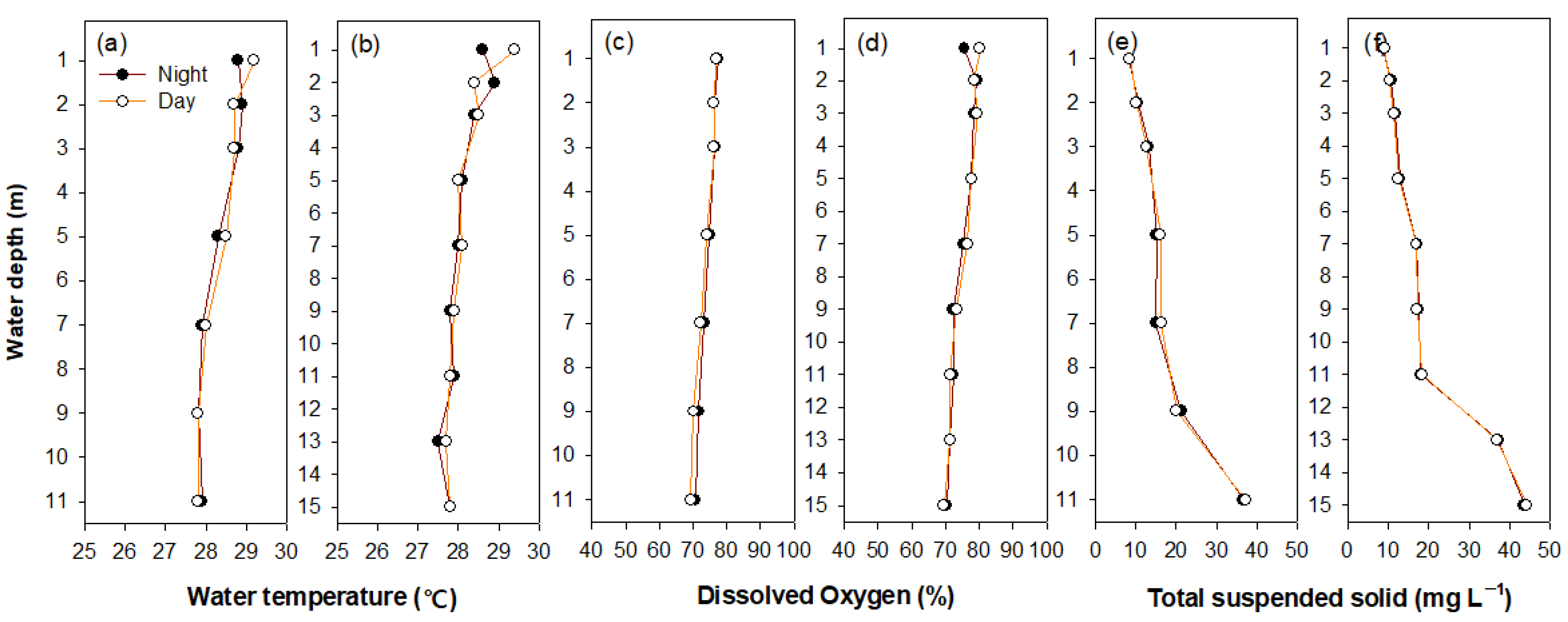
3.1. Environmental Variables and Cladocera Distributions

The environmental variables from each study site reflected the characteristics of temperate reservoirs (Table 1). The water depth, water temperatures, chlorophyll a, and pH were high in summer and low in winter (November–February), while DO showed a contrasting pattern (low in summer and high in winter). However, the seasonal patterns of TSS were relatively irregular. The seasonality of the environmental variables showed a similar pattern at all study sites.
The vertical gradient for some environmental variables (i.e., chlorophyll a and TSS) from the NRE was different in summer (one-way ANOVA, p < 0.05). The chlorophyll a concentration was higher in the upper layer than in the middle and bottom layers (one-way ANOVA, f = 2.016, p < 0.05), while the TSS was high in the bottom layer (one-way ANOVA, f = 3.347, p < 0.01). In particular, the TSS in the bottom layer showed a value that was approximately 4-fold higher than the upper layer. Furthermore, the chlorophyll a showed a difference of 6–15 µg∙mL−1 between the upper and bottom layers. Although the water temperature and DO were not statistically different between the layers, the upper layer showed a tendency toward higher water temperatures and DO than the middle and bottom layers. In contrast, the pH value was similar between each water layer. However, in the other seasons, i.e., excluding summer, the environmental variables were observed to have little variability between the water column layers.
The cladocerans were observed in spring, summer, and autumn, but not during winter; they were the most dominant in summer (Figure 2). A total of five cladoceran species (B. longirostris, D. obtusa, Diaphanozoma brachyrum, Bosminopsis deitersi, and Daphnia longispina) were identified at the sampling sites. The samples were dominated by B. longirostris and D. obtusa, and the other cladoceran densities were small (i.e., less than 20 individuals per L). The vertical distribution of cladocerans was varied with the seasons. In the summer, the cladocerans were more abundant in the upper and bottom layers than in the middle layer (i.e., in sites 1 and 3, one-way ANOVA, p < 0.05). However, in the autumn, a high density of cladocerans was found mainly in the upper layer. In contrast, we did not observe a different vertical distribution of cladocerans in spring. In contrast with sites 1 and 3, site 2 was very shallow (according to Table 1), thus it displayed minimal differences in the cladocerans’ vertical distribution.

3.2. Vertical Distribution of Two Cladocera Species between Day and Night in Summer

The monitored variables (i.e., water temperature, DO, and TSS) in each water layer showed minimal differences between day and night (Figure 3; one-way nested ANOVA, p > 0.05). Furthermore, the subgroups (i.e., three sampling points) for all of the environmental variables did not show statistical differences. Interestingly, the water temperatures and DO levels were observed to have a minimal difference between each of the water layers, while the TSS was higher in the bottom layer than in the upper and middle layers. Although the TSS values were similar in the upper and middle layers of each study site, the measurements differed at water layers below 9 and 11 m in sites 1 and 3, respectively.
The two dominant cladoceran species (B. longirostris and D. obtusa) presented different vertical distributions (Figure 4; Table 2). Bosmina longirostris was more abundant in the upper layer (1–3 m; site 1, 146 ind∙L–1; site 3, 121 ind∙L–1) during both the day and night, and presented low densities of under 31 ind∙L–1 below 4 m (Figure 4a,b). The vertical distribution of B. longirostris showed no significant difference between day and night (one-way nested ANOVA, p > 0.05). In contrast, D. obtusa presented statistically different vertical distributions between the day and night (Figure 4c,d; Table 2). During the day, D. obtusa remained mainly at depths of 9–11 m (93 ind∙L–1) and was rarely distributed in the upper layer. However, at night, most individuals were concentrated in the upper layer (73 ind∙L–1), while individuals were absent at depths of 9–11 m. The results of the one-way nested ANOVA indicated that the vertical distribution of D. obtusa was significantly different between day and night (Table 2). Moreover, the two cladoceran species showed homogeneous distributions between sampling points based on a one-way nested ANOVA.
The two cladoceran species showed different vertical distributions as a function of body size (Figure 5 and Figure 6). The vertical distribution of B. longirostris did not show a difference in body size, while for D. obtusa, a dramatic vertical difference was observed with body size. During the day, D. obtusa, with their larger body sizes, were mainly distributed in the bottom layer, while individuals with smaller body sizes remained in the upper layer. The Daphnia obtusa body length (μm) presented a significant relationship with the water layers (site 1, r2 = 0.71, p < 0.05; site 3, r2 = 0.75, p < 0.05). However, at night, the D. obtusa were mainly distributed in the upper layer (1–5 m), regardless of body size, and no individual was observed below 5 m (Figure 6). This vertical distribution pattern based on body size during the daytime was not found in B. longirostris. The vertical distribution of B. longirostris was not related to body size, either during the day or night (Figure 6).

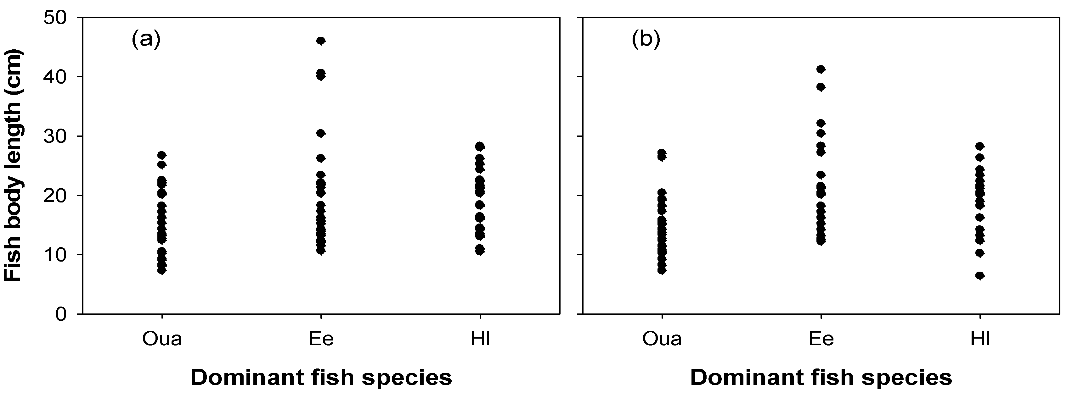
3.3. Fish Distribution in the Nakdong River Estuary

A total of 14 fish species were identified in the study sites (i.e., sites 1 and 3; Figure 7). Opsarichthys uncirostris amurensis was the most common species found at the study sites (site 1, 28.2%; site 3, 28.8%), followed by Erythroculter erythropterus (site 1, 24.1%; site 3, 28.8%) and Hemibarbus longirostris (site 1, 14.5%; site 3, 14.7%). The remaining fish species appeared to make up less than 5% of the communities. The abundance and number of fish species varied with the seasons. The fishes were more abundant in summer than other seasons, followed by spring and autumn. There was little difference in the abundance and number of fish species among the study sites (i.e., sites 1 and 3).
We found that the body lengths of the dominant fish species at the NRE (Figure 8) were similar. The body length of O. uncirostris amurensis ranged from 7.3 cm to 27.1 cm, similar to that of H. longirostris (6.4 cm to 28.3 cm). Compared to these species, E. erythropterus had a body length of 10.6 to 46 cm, approximately twice the body size. Although the body length of the dominant fishes varied between species, the body lengths of the three dominant fish species collected at the research sites were mostly less than 20 cm.
The consumption of D. obtusa by the dominant fish species was clearly different depending on the body length of the fish (Figure 9). Daphnia obtusa was mainly consumed by fish with body lengths of less than 20 cm (i.e., two size class; <10 cm and 10–20 cm). The Daphnia obtusa consumed by the small-sized fish (<20 cm) were mostly over 600 μm in size. Exceptionally, the consumption of D. obtusa by H. longirostris was seen mainly in populations less than 10 cm in length. In contrast, the high consumption of D. obtusa by O. uncirostris amurensis was undertaken not only by small (<10 cm) but also by bigger individuals (10–20 cm). We were not able to identify the consumption pattern of Erythroculter erythropterus because no individuals less than 10 cm were collected. The dominant fish species displayed a clear preference for D. obtusa over B. longirostris as a food source. We observed B. longirostris individuals only in the guts of O. uncirostris amurensis with body lengths of less than 10 cm. However, the dominant fish species with a body size of more than 20 cm (i.e., the two size classes of 20–30 cm and 30–40 cm) consumed not only B. longirostris but also D. obtusa as a food source.

4. Discussion

4.1. Seasonal Environmental Variables between Water Layers

Our study sites were in a desalted area due to the construction of an estuary barrage in 1987. The area is more like a lake or reservoir than a river due to the relatively deep water depth and slow flow rates present [38]. As such, the NRE has lost the environmental characteristics of river estuaries; instead, various features of lakes or reservoirs are present. Although not statistically significant, small differences between the water layers were observed in terms of water temperature and DO during the summer. However, the remaining factors (i.e., pH and chlorophyll a) showed minimal differences between the water layers. Vertical differences in these environmental variables (i.e., water temperature and DO) can be found mainly in lakes and reservoirs with large depths [39,40]. However, the difference in the water temperature or DO between the water layers at the NRE could not necessarily be classified as stratification. For the occurrence of stratification in the summer, water in the upper and bottom layers must be very stable [41] and the dense water in the bottom layer should not mix with the relatively light water of the surface layers. Water has the highest density at 4 °C but the water temperature and DO of the bottom layers at the estuary were not much different from the surface layers. From this finding, we supposed that the small difference in water temperature between the surface and bottom layers at the NRE was a result of temporarily elevated air temperatures in summer rather than stratification. The stable vertical distribution of water between the water layers requires a greater water depth than the maximum depth of the NRE [42]. This is because to keep the water temperature of the bottom layer close to 4 °C, the surface layer must have a minimal effect on it. This deeper water depth contributed to larger differences in DO between the upper and bottom layers. Most stratification associated with water temperature and DO mainly occurs in aquatic environments with a water depth of 20 to 30 m or more. However, the NRE has a water depth of less than 20 m (maximum depth of 15 m), thus environmental conditions (i.e., water depth) are not suitable for stratification to occur in the summer.
Although most of the environmental variables measured from the NRE were not significantly different between the water layers, there were very large differences in turbidity between the upper, middle, and bottom layers. Turbidity was the highest in the bottom layers. We surmise that this difference in turbidity between the water layers reflected the environmental characteristics of the Nakdong River Estuary. Considering that the study site is a river estuary, large amounts of dissolved substances from upstream areas and tributaries are likely to accumulate and summer rainfall may have led to an increase in turbidity in the study area. The NRE has less water flow and a relatively greater depth (site 1, 11 m; site 3, 15 m) than a common river such that turbidity can slowly sink to the bottom layers. This may result in a different habitat environment between the water layers, consequently affecting the spatial distribution of prey, such as cladoceran communities.

4.2. Vertical Distribution of Daphnia obtusa Due to Fish Predation

We speculated that the different vertical distribution was closely related to the occurrence of fish predation. Empirical studies suggest that the utilization of the bottom layers by D. obtusa during the day is a defensive behavior used to avoid fish predation [43,44]. During summer, the bottom layer of deeper lakes or reservoirs is not suitable for fish distribution as not only the water temperature and DO concentrations are lower than the surface layer but there is rarely an inflow of light into the water. Although it depends on the species, fish typically require more than 20–30% of DO and are rarely distributed in water layers below 20% DO [45]. The bottom layer is not suitable for the foraging activities of fish because there is little light coming in. As the bottom layer is avoided by fish, it can act as a refuge for the survival and stable population growth of the prey cladoceran species [46,47]. The food activity of fish is concentrated in the upper layers during the day when there is enough light [48]; therefore, the cladoceran communities can maintain their population by moving to the bottom layer to avoid predation [49]. However, since the bottom layer is supported by a lower food source (i.e., phytoplankton) than the upper layer [50], it is difficult for the cladocerans to inhabit the bottom layer for a long time. Hence, cladocerans move to the upper layer during the night for food and move back to the bottom layer during the day. This DVM pattern has frequently been identified in various deeper lakes and reservoirs [51,52]. Unfortunately, we found it difficult to apply these general rules in the NRE. For the bottom layer to become a place shunned by fish, the water temperatures and DO must be significantly lower than other water layers. However, the NRE has a relatively low water depth for these differences to occur.
Nevertheless, we assumed that the distribution of the fish species collected at the NRE was sufficient to cause different vertical distributions of D. obtusa during the day and night. Frequently appearing fishes at the NRE may well pose a threat to cladoceran communities. Previous studies have suggested that the dominant fishes in the estuary (i.e., O. uncirostris amurensis, E. erythropterus, and H. longirostris) utilize cladoceran species, including D. obtusa, as a food source [53,54]. Moreover, we have found that individuals of the dominant fish species that are less than 20 cm in size have been consuming D. obtusa at a higher rate. Most fish are visual predators and prefer easy-to-exploit individuals with relatively large body sizes that move frequently [55]. The negative effects of fish predation on cladocerans seem to have facilitated various defensive responses. In various studies, the DVM by cladocerans has been identified as an efficient defense response to avoid fish predation [56,57]. Moreover, it is one of the few major avoidance strategies utilized by cladocerans for their survival in fish-rich lakes and reservoirs.
We found that the utilization of bottom layers by D. obtusa during the day was not caused by the low water temperature and DO concentration of the bottom layer, as suggested in the previous study [58]. During the summer, the NRE did not show clear differences in water temperatures and DO between the water layers. From this finding, we surmise that turbidity, which was different between the water layers, might have facilitated the utilization of the bottom layer by D. obtusa. During the summer, turbidity was the highest in the bottom layers, and in such circumstances, fish cannot search for enough food. Hence, during the summer, the bottom layers appeared to be suitable for use as a refuge for D. obtusa to avoid fish predation. In the Nakdong River Estuary, sites 1 and 3 were observed to have a higher turbidity below 9 m and 11 m, respectively. In response, the density of D. obtusa was also relatively abundant at the bottom layers (i.e., 9 to 11 m and 11 to 15 m in sites 1 and 3, respectively) during the day. Although the NRE had an insufficient depth and climatic factors (i.e., high atmospheric temperatures were not persistent due to heavy summer rainfall and cloudy days [29]) for stratification, it appears that the high turbidity value in the bottom layers resulted in a different vertical distribution of D. obtusa during the day and night.

4.3. Behavioral Strategies by Body Size Class of the Two Cladoceran Species

The difference in predation experienced by the two cladoceran species strongly influenced their vertical distributions during the day and night. Daphnia obtusa is relatively preferred as prey because it has a larger size than B. longirostris [59]. Similarly, various empirical studies suggest that B. longirostris is not preferred by fishes because it has a relatively small body size [60]. Bosmina longirostris is more vulnerable to invertebrate predation, such as by copepods, than to predation by fish [61,62]. Thus, B. longirostris can often dominate rivers and streams supported by a high abundance of fishes [61]. In this study, we also observed distinct differences in body size between D. obtusa and B. longirostris. While the body size of D. obtusa ranged from 400 µm to 700 µm, B. longirostris body sizes were less than 400 μm. We supposed that the different body sizes of the two cladoceran species strongly influenced the foraging behavior of fishes. Bosmina longirostris, which is not consumed much by fishes, did not need to move to the bottom layers and was mainly distributed in the food-rich upper layer during both the day and night. From these results, we concluded that the body sizes of B. longirostris meant they were not significantly affected by fish predation.
In contrast, D. obtusa was seen to have different vertical distributions during the day that depended on body size. Daphnia obtusa, with a body size larger than 600 µm, was distributed in relatively deep water (i.e., bottom layer), while individuals smaller than 600 µm in size were found in the upper layer (i.e., approximately the uppermost 5 m). We speculated that D. obtusa that were smaller than 600 µm were mainly distributed in the upper layer during the day because they were not significantly affected by fish predation. In contrast, D. obtusa individuals larger than 600 µm in size were frequently consumed by fish, and thus they avoided predation by residing in the bottom layer during the day. We suggested that this differential vertical distribution of D. obtusa as a function of body size was an efficient behavioral strategy that co-evolved with the predation impact. Similarly, previous studies have described that the cladocerans community structure depends on the species or size class of the predatory fish. Amsinck et al. [63] suggested that the zooplanktivore brown trout, which was dominant in Lake Heygsvatn, played an important role in determining the community structure and richness of cladocerans. From this finding, we concluded that the different vertical distribution of cladoceran species that depended on body size was not a behavioral strategy that varied between the existence and absence of fish but rather was a defense strategy in individual cladocerans to predatory pressure gradients. Although we conducted the investigations only during the summer of 2013, the possibility cannot be ruled out that the small-sized D. obtusa that stayed on the upper layers during this summer may utilize the bottom layers to avoid fish predation if the body length of fish this summer was smaller than other seasons or the summer of the following years.
The behavioral strategy of cladoceran species to avoid fish predation can greatly contribute to the increase in the species abundance and diversity of cladoceran communities. Since the consumption of cladoceran by fish in lakes and reservoirs is a fast and active process, cladoceran communities are often extinct or exist with a very low density in these environments. Moreover, since aquatic ecosystems have a relatively small scale or are discontinuous compared to other ecosystems, the prey–predator interactions tend to occur at a greatly accelerated rate. From these findings, “refuge” utilization, such as the use of the bottom layer, can not only lower the predatory pressure but also contribute to the survival and the population growth of prey species. Moreover, this refuge presence has a positive effect in that by avoiding fish predation, it prevents population decline and ensures sustainable fecundity. Furthermore, the utilization of refuges by cladoceran species also leads to a continued food source for fish, contributing to the overall enhancement of biodiversity.

Author Contributions

The design of this research was equally shared between the authors. All authors contributed toward the conceptualization, methodology, and investigation. S.-K.K. contributed toward the development of the software and resources and wrote the original draft. J.-Y.C. contributed significantly to reviewing and editing the draft manuscript. All authors have read and agreed to the published version of the manuscript.

Funding

This research was supported by the Basic Science Research funded by the National Institute of Environmental Research (grant number: MONO1201731145).

Conflicts of Interest

The authors declare no conflict of interest.

References

  1. Curio, E. The Ethology of Predation; Springer Science & Business Media: New York, NY, USA, 2012. [Google Scholar]
  2. Dodson, S. Predator-induced reaction norms. Bioscience 1989, 39, 447–452. [Google Scholar] [CrossRef]
  3. Lima, S.L. Stress and decision making under the risk of predation: Recent developments from behavioral, reproductive, and ecological perspectives. In Advances in the Study of Behavior; Slater, P.J.B., Møller, A.P., Manfred, M., Eds.; Academic Press: London, UK, 1998; pp. 215–290. [Google Scholar]
  4. Pasternak, A.F.; Mikheev, V.N.; Wanzenböck, J. How plankton copepods avoid fish predation: From individual responses to variations of the life cycle. J. Ichthyol. 2006, 46, S220–S226. [Google Scholar] [CrossRef]
  5. Pettersson, L.B.; Nilsson, P.A.; Brönmark, C. Predator recognition and defence strategies in crucian carp, Carassius carassius. Oikos 2000, 88, 200–212. [Google Scholar] [CrossRef]
  6. Ángeles Esteban, M. An overview of the immunological defenses in fish skin. ISRN immunology 2012, 2012. [Google Scholar] [CrossRef] [Green Version]
  7. Luttbeg, B.; Sih, A. Predator and prey habitat selection games: The effects of how prey balance foraging and predation risk. Isr. J. Zool. 2004, 50, 233–254. [Google Scholar] [CrossRef] [Green Version]
  8. Sagrario, M.D.L.Á.G.; Balseiro, E. Indirect enhancement of large zooplankton by consumption of predacious macroinvertebrates by littoral fish. Arch. Hydrobiol. 2003, 158, 551–574. [Google Scholar] [CrossRef]
  9. Tollrian, R.; Harvell, C.D. The Ecology and Evolution of Inducible Defenses; Princeton University Press: Princeton, NJ, USA, 1999. [Google Scholar]
  10. Boeing, W.J.; Ramcharan, C.W.; Riessen, H.P. Clonal variation in depth distribution of Daphnia pulex in response to predator kairomones. Arch. Hydrobiol. 2006, 166, 241–260. [Google Scholar] [CrossRef]
  11. Ringelberg, J. The photobehaviour of Daphnia spp. as a model to explain diel vertical migration in zooplankton. Biol. Rev. 1999, 74, 397–423. [Google Scholar] [CrossRef]
  12. Walls, M.; Ketola, M. Effects of predator-induced spines on individual fitness in Daphnia pulex. Limnol. Oceanogr. 1989, 34, 390–396. [Google Scholar] [CrossRef]
  13. Haupt, F.; Stockenreiter, M.; Baumgartner, M.; Boersma, M.; Stibor, H. Daphnia diel vertical migration: Implications beyond zooplankton. J. Plankton Res. 2009, 31, 515–524. [Google Scholar] [CrossRef] [Green Version]
  14. Loose, C.J. Lack of endogenous rhythmicity in Daphnia diel vertical migration. Limnol. Oceanogr. 1993, 38, 1837–1841. [Google Scholar] [CrossRef]
  15. Ringelberg, J. A mechanism of predator-mediated induction of diel vertical migration in Daphnia hyalina. J. Plankton Res. 1991, 13, 83–89. [Google Scholar] [CrossRef]
  16. Battes, K.P.; Momeu, L. Diel vertical distribution of planktonic microcrustaceans (Crustacea: Cladocera, Copepoda) in a natural shallow lake from Transylvania, Romania. J. Limnol. 2014, 73, 34–44. [Google Scholar] [CrossRef] [Green Version]
  17. Jung, J.; Hojnowski, C.; Jenkins, H.; Ortiz, A.; Brinkley, C.; Cadish, L.; Evans, A.; Kissinger, P.; Ordal, L.; Osipova, S.; et al. Diel vertical migration of zooplankton in Lake Baikal and its relationship to body size. In Ecosystems and Natural Resources of Mountain Regions; Smirnov, A.I., Izmest’eva, L.R., Eds.; Nauka: Novosibirsk, Rusia, 2004; pp. 131–140. [Google Scholar]
  18. Semyalo, R.; Nattabi, J.K.; Larsson, P. Diel vertical migration of zooplankton in a eutrophic bay of Lake Victoria. Hydrobiologia 2009, 635, 383–394. [Google Scholar] [CrossRef] [Green Version]
  19. Brancelj, A.; Blejec, A. Diurnal vertical migration of Daphnia hyalina Leydig, 1860 (Crustacea: Cladocera) in Lake Bled (Slovenia) in relation to temperature and predation. Hydrobiologia 1994, 284, 125–136. [Google Scholar] [CrossRef]
  20. Degefu, F.; Schagerl, M. Zooplankton abundance, species composition and ecology of tropical high-mountain crater Lake Wonchi, Ethiopia. J. limnol. 2015, 74, 324–334. [Google Scholar] [CrossRef]
  21. Easton, J.; Gophen, M. Diel variation in the vertical distribution of fish and plankton in Lake Kinneret: A 24-h study of ecological overlap. Hydrobiologia 2003, 491, 91–100. [Google Scholar] [CrossRef]
  22. Johnsen, G.J.; Jakobsen, P.J. The effect of food limitation on vertical migration in Daphnia longispina. Limnol. Oceanogr. 1987, 32, 873–880. [Google Scholar] [CrossRef]
  23. Ringelberg, J.; Van Gool, E. On the combined analysis of proximate and ultimate aspects in diel vertical migration (DVM) research. Hydrobiologia 2003, 491, 85–90. [Google Scholar] [CrossRef]
  24. De Bernardi, R.; Giussani, G.; Manca, M. Cladocera: Predators and prey. In Cladocera; Forró, L., Frey, D.G., Eds.; Springer: Dordrecht, The Netherlands, 1987; pp. 225–243. [Google Scholar]
  25. Ramos-Jiliberto, R.O.D.R.I.G.O.; Zúñiga, L.R. Depth-selection patterns and diel vertical migration of Daphnia ambigua (Crustacea: Cladocera) in lake El Plateado. Rev. Chil. Hist. Nat. 2001, 74, 573–585. [Google Scholar] [CrossRef]
  26. Horppila, J.; Malinen, T.; Nurminen, L.; Tallberg, P.; Vinni, M. A metalimnetic oxygen minimum indirectly contributing to the low biomass of cladocerans in Lake Hiidenvesi–a diurnal study on the refuge effect. Hydrobiologia 2000, 436, 81–90. [Google Scholar] [CrossRef]
  27. Ha, K.; Cho, E.A.; Kim, H.W.; Joo, G.J. Microcystis bloom formation in the lower Nakdong River, South Korea: Importance of hydrodynamics and nutrient loading. Mar. Freshw. Res. 1999, 50, 89–94. [Google Scholar] [CrossRef]
  28. Kim, H.W.; Joo, G.J.; Walz, N. Zooplankton Dynamics in the Hyper-Eutrophic Nakdong River System (Korea) Regulated by an Estuary Dam and Side Channels. Internat. Rev. Hydrobiol. 2001, 86, 127–143. [Google Scholar] [CrossRef]
  29. Choi, J.Y.; Jeong, K.S.; Kim, H.W.; Chang, K.H.; Joo, G.J. Inter-annual variability of a zooplankton community: The importance of summer concentrated rainfall in a regulated river ecosystem. J. Ecol. Environ. 2011, 34, 49–58. [Google Scholar] [CrossRef] [Green Version]
  30. Jeong, K.S.; Kim, D.K.; Joo, G.J. Delayed influence of dam storage and discharge on the determination of seasonal proliferations of Microcystis aeruginosa and Stephanodiscus hantzschii in a regulated river system of the lower Nakdong River (South Korea). Water Res. 2007, 41, 1269–1279. [Google Scholar] [CrossRef]
  31. An, J.H.; Lee, K.H. Correlation and hysteresis analysis of air-water temperature in four rivers: Preliminary study for water temperature prediction. J. Environ. Policy 2013, 12, 17–32. [Google Scholar]
  32. Wetzel, R.G.; Likens, G.E. Composition and biomass of phytoplankton. In Limnological Analyses; Springer: New York, NY, USA, 2000; pp. 147–174. [Google Scholar]
  33. Haney, J.F.; Hall, D.J. Sugar-coated Daphnia: A preservation technique for Cladocera 1. Limnol. Oceanogr. 1973, 18, 331–333. [Google Scholar] [CrossRef]
  34. Mizuno, T.; Takahashi, E. An Illustration Guide to Freshwater Zooplankton in Japan; Tokai University: Tokyo, Japan, 1999. [Google Scholar]
  35. Kim, I.S.; Choi, Y.; Lee, C.L.; Lee, Y.J.; Kim, B.J.; Kim, J.H. Illustrated Book of Korean Fishes; Kyohak Publishing: Seoul, Korea, 2005. [Google Scholar]
  36. Javahery, S.; Nekoubin, H.; Moradlu, A.H. Effect of anaesthesia with clove oil in fish. Fish Physiol. Biochem. 2012, 38, 1545–1552. [Google Scholar] [CrossRef]
  37. Hurlbert, S.H. Pseudoreplication and the design of ecological field experiments. Ecol. Monogr. 1984, 54, 187–211. [Google Scholar] [CrossRef] [Green Version]
  38. Yoon, J.D.; Jang, M.H.; Jo, H.B.; Jeong, K.S.; Kim, G.Y.; Joo, G.J. Changes of fish assemblages after construction of an estuary barrage in the lower Nakdong River, South Korea. Limnology 2016, 17, 183–197. [Google Scholar] [CrossRef]
  39. Read, J.S.; Hamilton, D.P.; Jones, I.D.; Muraoka, K.; Winslow, L.A.; Kroiss, R.; Wu, C.H.; Gaiser, E. Derivation of lake mixing and stratification indices from high-resolution lake buoy data. Environ. Model. Softw. 2011, 26, 1325–1336. [Google Scholar] [CrossRef]
  40. Kraemer, B.M.; Anneville, O.; Chandra, S.; Dix, M.; Kuusisto, E.; Livingstone, D.M.; Rimmer, A.; Schladow, S.G.; Silow, E.; Sitoki, L.M.; et al. Morphometry and average temperature affect lake stratification responses to climate change. Geophys. Res. Lett. 2015, 42, 4981–4988. [Google Scholar] [CrossRef] [Green Version]
  41. Berger, S.A.; Diehl, S.; Stibor, H.; Trommer, G.; Ruhenstroth, M. Water temperature and stratification depth independently shift cardinal events during plankton spring succession. Glob. Chang. Biol. 2010, 16, 1954–1965. [Google Scholar] [CrossRef]
  42. Hassan, H.; Aramaki, T.; Hanaki, K.; Matsuo, T.; Wilby, R. Lake stratification and temperature profiles simulated using downscaled GCM output. Water Sci. Technol. 1998, 38, 217–226. [Google Scholar] [CrossRef]
  43. Lampert, W. Ultimate causes of diel vertical migration of zooplankton: New evidence for the predator-avoidance hypothesis. Arch. Hydrobiol Beih. Ergebn. Limnol. 1993, 39, 79–88. [Google Scholar]
  44. Von Elert, E.; Loose, C.J. Predator-induced diel vertical migration in Daphnia: Enrichment and preliminary chemical characterization of a kairomone exuded by fish. J. Chem. Ecol. 1996, 22, 885–895. [Google Scholar] [CrossRef]
  45. Decker, M.B.; Breitburg, D.L.; Purcell, J.E. Effects of low dissolved oxygen on zooplankton predation by the ctenophore Mnemiopsis leidyi. Mar. Ecol. Prog. Ser. 2004, 280, 163–172. [Google Scholar] [CrossRef]
  46. Horppila, J.; Eloranta, P.; Liljendahl-Nurminen, A.; Niemistö, J.; Pekcan-Hekim, Z. Refuge availability and sequence of predators determine the seasonal succession of crustacean zooplankton in a clay-turbid lake. Aquat. Ecol. 2009, 43, 91–103. [Google Scholar] [CrossRef]
  47. Choi, J.Y.; Jeong, K.S.; La, G.H.; Joo, G.J.; Kim, J.; Kim, S.J.; Kim, S.H.; Chung, Y.H.; Kim, D.K.; Do, Y.; et al. Spatio-temporal distribution of Diaphanosoma brachyurum (Cladocera: Sididae) in freshwater reservoir ecosystems: Importance of maximum water depth and macrophyte beds for avoidance of fish predation. J. Limnol. 2015, 74, 403–413. [Google Scholar] [CrossRef] [Green Version]
  48. Regular, P.M.; Hedd, A.; Montevecchi, W.A. Fishing in the dark: A pursuit-diving seabird modifies foraging behaviour in response to nocturnal light levels. PLoS ONE 2011, 6, e26763. [Google Scholar] [CrossRef]
  49. Seitz, F.; Bundschuh, M.; Rosenfeldt, R.R.; Schulz, R. Nanoparticle toxicity in Daphnia magna reproduction studies: The importance of test design. Aquat. Toxicol. 2013, 126, 163–168. [Google Scholar] [CrossRef]
  50. Gaevsky, N.A.; Zotina, T.A.; Gorbaneva, T.B. Vertical structure and photosynthetic activity of Lake Shira phytoplankton. Aquat. Ecol. 2002, 36, 165–178. [Google Scholar] [CrossRef]
  51. Lampert, W. The adaptive significance of diel vertical migration of zooplankton. Funct. Ecol. 1989, 3, 21–27. [Google Scholar] [CrossRef]
  52. Pearre, S. Eat and run? The hunger/satiation hypothesis in vertical migration: History, evidence and consequences. Biol. Rev. 2003, 78, 1–79. [Google Scholar] [CrossRef]
  53. Mitchell, M.J.; Mills, E.L.; Idrisi, N.; Michener, R. Stable isotopes of nitrogen and carbon in an aquatic food web recently invaded by (Dreissena polymorpha)(Pallas). Can. J. Fish. Aquat. Sci. 1996, 53, 1445–1450. [Google Scholar] [CrossRef]
  54. Fry, B.; Mumford, P.L.; Tam, F.; Fox, D.D.; Warren, G.L.; Havens, K.E.; Steinman, A.D. Trophic position and individual feeding histories of fish from Lake Okeechobee, Florida. Can. J. Fish. Aquat. Sci. 1999, 56, 590–600. [Google Scholar] [CrossRef]
  55. Ibrahim, A.A.; Huntingford, F.A. The role of visual cues in prey selection in three-spined sticklebacks (Gasterosteus aculeatus). Ethology 1989, 81, 265–272. [Google Scholar] [CrossRef]
  56. Thys, I.; Hoffmann, L. Diverse responses of planktonic crustaceans to fish predation by shifts in depth selection and size at maturity. Hydrobiologia 2005, 551, 87–98. [Google Scholar] [CrossRef]
  57. Wojtal-Frankiewicz, A.; Frankiewicz, P.; Jurczak, T.; Grennan, J.; McCarthy, T.K. Comparison of fish and phantom midge influence on cladocerans diel vertical migration in a dual basin lake. Aquat. Ecol. 2010, 44, 243–254. [Google Scholar] [CrossRef]
  58. Mehner, T.; Hölker, F.; Kasprzak, P. Spatial and temporal heterogeneity of trophic variables in a deep lake as reflected by repeated singular samplings. Oikos 2005, 108, 401–409. [Google Scholar] [CrossRef]
  59. Jeschke, J.M.; Tollrian, R. Prey swarming: Which predators become confused and why? Anim. Behav. 2007, 74, 387–393. [Google Scholar] [CrossRef]
  60. Uusitalo, L.; Horppila, J.; Eloranta, P.; Liljendahl-Nurminen, A.; Malinen, T.; Salonen, M.; Vinni, M. Leptodora kindti and flexible foraging behaviour of fish–factors behind the delayed biomass peak of cladocerans in Lake Hiidenvesi. Internat. Rev. Hydrobiol. 2003, 88, 34–48. [Google Scholar] [CrossRef]
  61. Chang, K.H.; Hanazato, T. Seasonal and spatial distribution of two Bosmina species (B. longirostris and B. fatalis) in Lake Suwa, Japan: Its relation to the predator Leptodora. Limnology 2003, 4, 0047–0052. [Google Scholar] [CrossRef]
  62. Labaj, A.L.; Korosi, J.B.; Kurek, J.; Jeziorski, A.; Keller, W.; Smol, J.P. Response of Bosmina size structure to the acidification and recovery of lakes near Sudbury. Can. J. Limnol. 2016, 75, 22–29. [Google Scholar] [CrossRef] [Green Version]
  63. Amsinck, S.L.; Strzelczak, A.; Bjerring, R.; Landkildehus, F.; Lauridsen, T.L.; Christoffersen, K.; Jeppesen, E. Lake depth rather than fish planktivory determines cladoceran community structure in Faroese lakes–evidence from contemporary data and sediments. Freshw. Biol. 2006, 51, 2124–2142. [Google Scholar] [CrossRef]
Figure 1. Map of the study area in the Nakdong River estuary. The study sites are indicated as solid circles (●). The inset map in the lower-left corner indicates the estuary’s location in the Korean Peninsula.
Water 12 02154 g001
Figure 2. Seasonal vertical distribution of cladocerans in the Nakdong River Estuary. Spring (ac), summer (df), and autumn (gi) for sites 1, 2, and 3.
Water 12 02154 g002
Figure 3. The vertical distributions (at intervals of 1–2 m) of water temperature (a,b), dissolved oxygen (c,d), and total suspended solids (e,f) between day and night at sites 1 (a,c,e) and 3 (b,d,f).
Water 12 02154 g003
Figure 4. The vertical distribution (at intervals of 1–2 m) of Bosmina longirostris (a,b) and Daphnia obtusa (c,d) between day and night at sites 1 (a,c) and 3 (b,d).
Water 12 02154 g004
Figure 5. The relationship between body length (μm) of Bosmina longirostris and water depth during the daytime at sites 1 (a) and 3 (b) and during the night at sites 1 (c) and 3 (d).
Water 12 02154 g005
Figure 6. The relationship between body length (μm) of Daphnia obtusa and water depth during the daytime at sites 1 (a) and 3 (b) and during the night at sites 1 (c) and 3 (d).
Water 12 02154 g006
Figure 7. Seasonal abundance and number of fish species collected from sites 1 (a) and 3 (b).
Water 12 02154 g007
Figure 8. The body lengths of the three dominant species of fish collected from sites 1 (a) and 3 (b) during summer. Oua, Opsarichthys uncirostris amurensis; Ee, Erythroculter erythropterus; Hl, Hemibarbus longirostris.
Water 12 02154 g008
Figure 9. Consumption and body size of Daphnia obtusa in the guts of three species of fish during summer at sites 1 (ac) and 3 (df): Opsarichthys uncirostris amurensis (a,d), Erythroculter erythropterus (b,e), and Hemibarbus longirostris (c,f).
Water 12 02154 g009
Table 1. Seasonal environmental variables at each site of the Nakdong River Estuary. Depth, Water depth (m); WT, Water temperature (°C); DO, Dissolved oxygen (%); Chl. a, Chlorophyll a (µg∙L–1); TSS, Total suspended solids (mg∙L–1); U, Upper Layer; M, Middle Layer; B, Bottom Layer.
MonthVariablesSite 1Site 2Site 3
UMBUMBUMB
Feb.Depth1381131512
WT5.35.05.15.05.65.35.55.35.1
DO129.7123.9123.9129.0124.6123.7136.0125.7124.6
pH6.205.845.916.186.886.458.526.286.94
Chl. a22.413.314.712.610.58.48.410.59.8
TSS10.011.015.08.08.211.011.012.419.0
MayDepth1591231713
WT18.018.318.118.218.317.918.018.718.1
DO87.389.989.590.994.191.987.390.690.8
pH5.585.435.465.415.455.425.585.876.05
Chl. a12.016.016.012.016.016.012.012.016.0
TSS4.44.45.65.45.85.97.16.97.6
Aug.Depth15111351715
WT29.128.027.829.128.928.029.228.328.0
DO74.572.970.775.073.573.277.274.871.4
pH7.307.147.307.227.106.557.667.687.60
Chl. a40.037.034.532.237.030.556.049.740.8
TSS9.616.037.29.618.834.48.016.843.6
Nov.Depth1591241713
WT12.912.111.612.912.111.712.912.210.8
DO93.294.094.992.893.295.095.693.096.1
pH7.377.847.978.078.128.097.357.557.41
Chl. a5.54.15.32.92.93.05.44.14.8
TSS4.56.36.75.35.55.710.88.87.9
Table 2. One-way nested ANOVA results for the effects of the main groups (shown as “Time” in the table: daytime and night) and subgroups (i.e., shown as “Sampling point”) on two cladoceran species. df, Degrees of Freedom. Statistically significant values are indicated in bold.
SpeciesSiteVariancedfFp
B. longirostrisSite 1Time11.5430.098
Sampling point40.4321.753
Site 3Time11.6320.086
Sampling point40.6421.629
D. obtusaSite 1Time114.24<0.01
Sampling point40.1410.943
Site 3Time112.41<0.01
Sampling point40.1500.911

