An Enhanced Approach to the Spatial and Statistical Analysis of Factors Influencing Spring Distribution on a Transboundary Karst Aquifer

Abstract

Karst aquifers are indispensable, yet vulnerable, resources; therefore, they require a comprehensive protection strategy. Since springs are the terminal points of the karst flow systems, knowledge of their distribution is a key element for the better understanding of groundwater flow, availability and vulnerability. The present study aims to introduce a data-driven analysis by the application of a spatial statistical technique (Weights of Evidence (WofE)) for the evaluation of factors influencing spring distribution in karst areas. A workflow was developed for investigating two questions: where will the springs locate, and where will the permanent springs evolve? This workflow has the potential for application to unconfined karst areas. This enhanced approach was applied to an unconfined transboundary aquifer, the Gömör–Torna Karst (HU and SK). The roles of five factors was statistically investigated: terrain elevation, distance to faults, distance of the carbonate–non-carbonate rock contact, distance to sinkholes, and precipitation distribution. The validation procedures confirmed the effectiveness of the approach. The resulting predictive maps are useful for decision-makers to delineate areas holding potential karst springs and to address water availability problems and protection measures. In addition, the WofE technique improved the comprehension of the geological conditions favourable for the formation of the springs.

1. Introduction

Karst aquifers store indispensable water resources. On a global level, about 20–25% of the population depends partially or entirely on karst water resources [1]. Shallow karsts can be characterised as having a distinctive flow system: spatially changing hydraulic conductivity, duality in recharge, porosity, flow, and storage [2]. Due to these features, contaminants can easily reach the groundwater table and the springs, and they can be transported through karstic conduits over large distances. The short residence time and limited interaction with the material of the aquifer cause inefficiency in filtration, adsorption, and chemical and microbiological decay in karst systems [3]. Besides the quality of karst water resources, their quantity and availability might also be altered, due to the climatic changes in precipitation patterns and evaporation [4,5,6,7]. Therefore, they are highly vulnerable drinking water resources, requiring the right protection strategies. These need to be based on the understanding of flow systems.

Springs distribution is very relevant for better understanding not only of the flow, but of the karstic features, and the groundwater vulnerability as well [1,3,8,9,10,11,12,13]. Karst springs can be permanent or, often, temporary. Permanent springs feed stream flows through the entire year, whilst temporary springs become dry at times or even most of the year. Temporary springs flow at irregular intervals, related to the changes of groundwater level, which is controlled by the variations in rainfall and snow melt [14]. Despite their global significance and abundance, temporary springs have been understudied for long time [15].

For the purpose of modelling spatially related questions in geosciences, GIS-based statistical techniques, such as logistic regression, conditional (i.e., Bayesian) probability, fuzzy logic, artificial neural networks, discriminant analysis and likelihood ratio functions are frequently used [16]. The Weights of Evidence (WofE) is a well-known spatial statistical method, which combines different spatial datasets in a GIS environment to analyse and describe their interactions and generate predictive patterns [17]. It has been successfully applied for the purpose of mineral exploration [17,18], landslide hazard zonation (e.g., [19]), groundwater productivity potential (e.g., [20]), groundwater spring potential (e.g., [21,22]) and vulnerability assessment (e.g., [23,24]).

The WofE technique is applied in this study for the evaluation of factors influencing spring distribution in karst areas. The developed workflow for the analysis of the spring distribution can be widely used on unconfined karst areas, and it is presented on the example of the Gömör–Torna Karst (also known as the Aggtelek Karst and Slovak Karst). This study site is an unconfined transboundary aquifer found on the border of Hungary and Slovakia. In the past decades, the Gömör–Torna Karst was the focus of numerous studies, including hydrogeological investigations and local-scale groundwater vulnerability assessments (e.g., [25,26,27,28,29]). Thanks to these studies, a unique, long-term, detailed hydrometeorological database [30] was available, providing an appropriate basis for the testing and validation of the data-driven analysis. Moreover, this transboundary aquifer has significant shared karst water resources and has a high natural conservation value; therefore, understanding its flow processes is highly necessary.

By means of the WofE technique, we investigated two main questions: Q1—where will the springs locate and Q2—where will the temporary and permanent springs evolve? Looking forwards, future research might extend the explanations of factors influencing groundwater vulnerability.

2. Proposed Methodology

2.1. Weights of Evidence Technique

The Weights of Evidence technique is a spatial statistical method based on Bayesian conditional probability, which enables observations of the individual roles and the combined effect of different geological, geophysical, and geochemical features, to assess the spatial distribution of a natural phenomenon [17]. The occurrences of the phenomenon are defined as the response variable, whilst factors influencing their presence and distribution in the study area are called evidential themes. The response variable and the evidential themes are combined to generate predictive probability maps (response themes). The mathematical description and a detailed discussion of assumptions and limitations of the WofE technique have been described in several works [17,18,23]. We report here a brief review of the steps and mathematical operations.

Table 1. Relevant concepts of the WofE technique and their operative applications in natural resources fields.

Concept	Definition	Operative Translation in...
Response variable	The phenomenon under consideration (e.g., mineral deposits). The location of occurrences is known. The occurrences are treated as points. Occurrences are subdivided into two sets used for generating the response themes (training set) or performing calibration and validation processes (control set) [17,18].	Examples: mineral deposits (e.g., [17]), landslides (e.g., [19]), contaminated water wells (e.g., [23,31]). Occurrences can be either training points (TPs), being part of the training set, or control points (CPs), as part of the control set.
Evidential themes or predictors	Factors influencing the location and spatial distribution of the response variable. Evidential themes represent sets of continuous or categorical spatial data [17,18].	Geological, geomorphological and physical factors influencing the presence and spatial distribution of the phenomenon under consideration, for example: - proximity to hydrothermal areas, distance to faults or folds, geochemical anomalies distribution for mineral exploration [17,18]; - altitude, slope, aspect, lithology of surface rocks and deposits, distance to fault, land use for landslides hazard zonation (e.g., [19]); - groundwater depth, hydraulic conductivity, precipitation, land use for groundwater vulnerability assessments (e.g., [23,31]).
Response theme or predictive probability map	The response theme (i.e., predictive probability map) is the result of the WofE [32].	A response theme (i.e., predictive probability map) is an output data layer showing the distribution of posterior probability values [32]. It represents the relative probability of occurrence of the phenomenon under consideration (e.g., presence of mineral deposits, landslides risk, groundwater vulnerability).
Prior probability	The probability that a unit area contains an occurrence without considering any evidential themes [17,18].	It is given by the ratio between the number of unit areas containing a TP and the total area [17].
Posterior probability	The posterior probability represents the relative probability that a unit area contains an occurrence based on the evidences provided by the evidential themes [17,18].	The posterior probability is calculated by adding a weight for each evidence class to the logit of the prior probability and converting the sum from logit to probability [17].
Generalization of the evidential themes	Ordered evidential themes can be generalized during the analysis to improve model results relating the number and location of TPs and the presence of random effects [32].	Generalizing an ordered evidential theme means defining ranges of values that can be grouped into evidence classes, which have a statistically significant spatial correlation with the location of TPs [32]. An objective (semi-guided) procedure has been developed by Sorichetta, Masetti, Ballabio and Sterlacchini [16].
Weights	Weights establish a spatial association between TPs and evidential themes. Weights are the values assigned to each evidence class [18,32].	Weights are calculated for each evidential theme based on the presence or absence of TPs [18,32]: - a positive weight (W+) is calculated for areas that have more TPs than expected by chance; - a negative weight (W−) is calculated for areas that have fewer TPs than expected by chance; - a weight of zero means that there is no association between TPs and the evidential theme, or that the evidential theme is not a discriminating factor.
Contrast	The contrast is a measure of the usefulness of each evidence class in predicting the location of the occurrences [17,18].	For each class of each evidential theme, the contrast is calculated as the difference between the positive and the negative weight (C = W+ − W−). A positive contrast value means a direct correlation between the class and the TPs, and a negative value means an indirect correlation, whereas a value close to zero means low or no correlation [18]
Statistical significance	A level of significance needs to be established prior the generalization process. This is equivalent to a Student t-test [18,23].	A confidence value for the ratio between the contrast and its standard deviation (i.e., normalized contrast) must be selected to provide a useful measure of the significance of the contrast and, thus, to the respective class of an evidential theme. See [23], for a complete list of confidence values and relative test values.
Scientific explanation	The pattern distribution of an evidential theme after the generalization process needs some justification by scientific reasoning [16,18,19,23,31,33].	The pattern distribution needs to be justifiable from either a geological (e.g., [34]), geomorphological (e.g., [19]) or hydrogeological (e.g., [31]) point of view.
Bias	Statistical models generally require the use of random samples of a population. A bias could occur when the spatial distribution of occurrences differs greatly from an ideal random setting. Such condition could occur in mineral exploration researches or hydrogeological studies. For example, sources of exploration bias include land accessibility factors (location of outcrops, roads, lakes, swamps, property boundaries, political boundaries, etc.) and perceived exploration criteria (faults, alteration, geochemical anomalies, etc.); in most hydrogeological settings, biased distribution of monitoring wells is due to land accessibility factors and a tendency to site more monitoring wells in known contaminated areas than in other areas [35,36].	Sorichetta, Masetti, Ballabio and Sterlacchini [16] developed a quantitative methodology that allows sampling bias to be recognized and contrast values to be corrected for sampling bias effects in hydrogeological studies. In an ideal random setting, contrasts calculated using all occurrences (both TPs and CPs) should have values of near zero for all evidence classes. If a bias occurs, the contrast is adjusted by subtracting the contrast calculated using all occurrences from the contrast calculated using either a) the TPs or b) the CPs. This procedure requires that the same classification of the Evidential Themes is used for both the analyses with all occurrences and either the TPs or the CPs.
Reclassified Predictive Probability Map	Scientifically defensible response themes, expressed as probability maps, require additional interpretation before being usable for most of the end-user purposes. This is due to the excessive number of classes, which is inappropriate in practical purposes (e.g., land use regulations) [37,38,39].	Sorichetta, Masetti, Ballabio, Sterlacchini and Beretta [38], in their study on groundwater vulnerability assessment, have demonstrated the reliability and suitability of the geometrical interval classification method for reclassifying posterior probability values and obtain maps consisting of few classes (5). The geometrical interval classification method which ensures that each class has approximately the same number of different post probability values.
Calibration & Validation	The meaningfulness, reliability and accuracy of the probability maps need to be checked to improve defensibility of the results and facilitate implementation [19,23,38,40].	Techniques: (a) Area-under-the-curve (AUC) and Success Rate Curve methods, on posterior probability values [40]; (b) Frequency of TPs and CPs, on reclassified predictive probability maps [38]; (c) Density of CPs, on reclassified predictive probability maps [38].

provides a list of the relevant concepts of the WofE technique, their theoretical definitions, and their operative applications in several geological, geomorphological, and hydrogeological fields.

The WofE calculations involve the following steps: (I) evaluation of the prior probability; (II) calculation of the positive and negative weights, as well as the contrasts and normalised contrasts; (III) calculation of the posterior probability.

(I) The study area is subdivided into unit cells of the same extent. The extension of a unit area needs to be small enough to contain only one occurrence (i.e., spring). Prior probability is defined by the ratio between the cells holding the occurrences (i.e., the number of cells containing an occurrence, D) and the total area (i.e., the total number of cells):

$$P_{prior}=\frac{N_D}{N_T}$$

(1)

where N_D and N_T are, respectively, the number of cells containing an occurrence, and the total number of cells in the study area.

(II) Each evidential theme is categorized in classes and for each class a positive and a negative weight are computed on the basis of the location of the occurrences with respect to the study area. Thus, for a given class B, the positive weight W⁺ and the negative weight W⁻ would be higher and lower than zero. The resulting combination depends on whether B has more or fewer occurrences than we would expect by chance. The weights can be expressed as:

$$W^{+}=\frac{P\left\{B|D\right\}}{P\left\{B|\overline{D}\right\}}$$

(2)

$$W^{-}=\frac{P\left\{\overline{B}|D\right\}}{P\left\{\overline{B}|\overline{D}\right\}}$$

(3)

where $P\left\{B|D\right\}$ is the probability of a cell being in the class B when the same cell contains an occurrence, $P\left\{B|\overline{D}\right\}$ is the probability of a cell being in the class B when the same cell does not contain an occurrence, $P\left\{\overline{B}|D\right\}$ is the probability of a cell not being in the class B when it contains an occurrence, and $P\left\{\overline{B}|\overline{D}\right\}$ is the probability of a cell not being in the class B when it does not contain an occurrence. In order for a class—and, thus, for the evidential theme—to be statistically significant, a confidence value must be established. The confidence value is compared to the normalised contrast calculated for each class of a given evidential theme, as the ratio between the contrast (W⁺ minus W⁻) and its standard deviation.

(III) The posterior probability represents the relative probability that a cell contains an occurrence on the basis of the evidence provided by the evidential themes (i.e., on the basis of the calculated weights and the proof of being statistically significant). The posterior probability can be expressed as:

$$O\left\{D|B_1^k{\displaystyle \cap }{B}_2^k{\displaystyle \cap }{B}_3^k\dots {\displaystyle \cap }{B}_n^k\right\}={\displaystyle \sum }_{j=1}^n{W}_j^k+O\left\{D\right\}$$

(4)

where n identifies each single class used to categorise each evidential theme, k is either “+” or “−“, depending on whether the prediction spatial class, B_n, is either present or absent, and O is the odds form of the probability that a cell within the study area contains an occurrence.

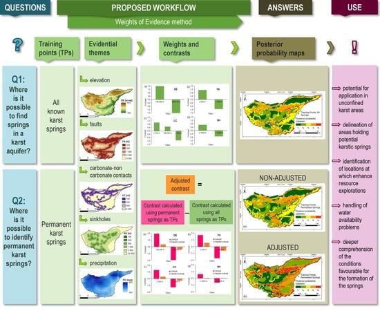
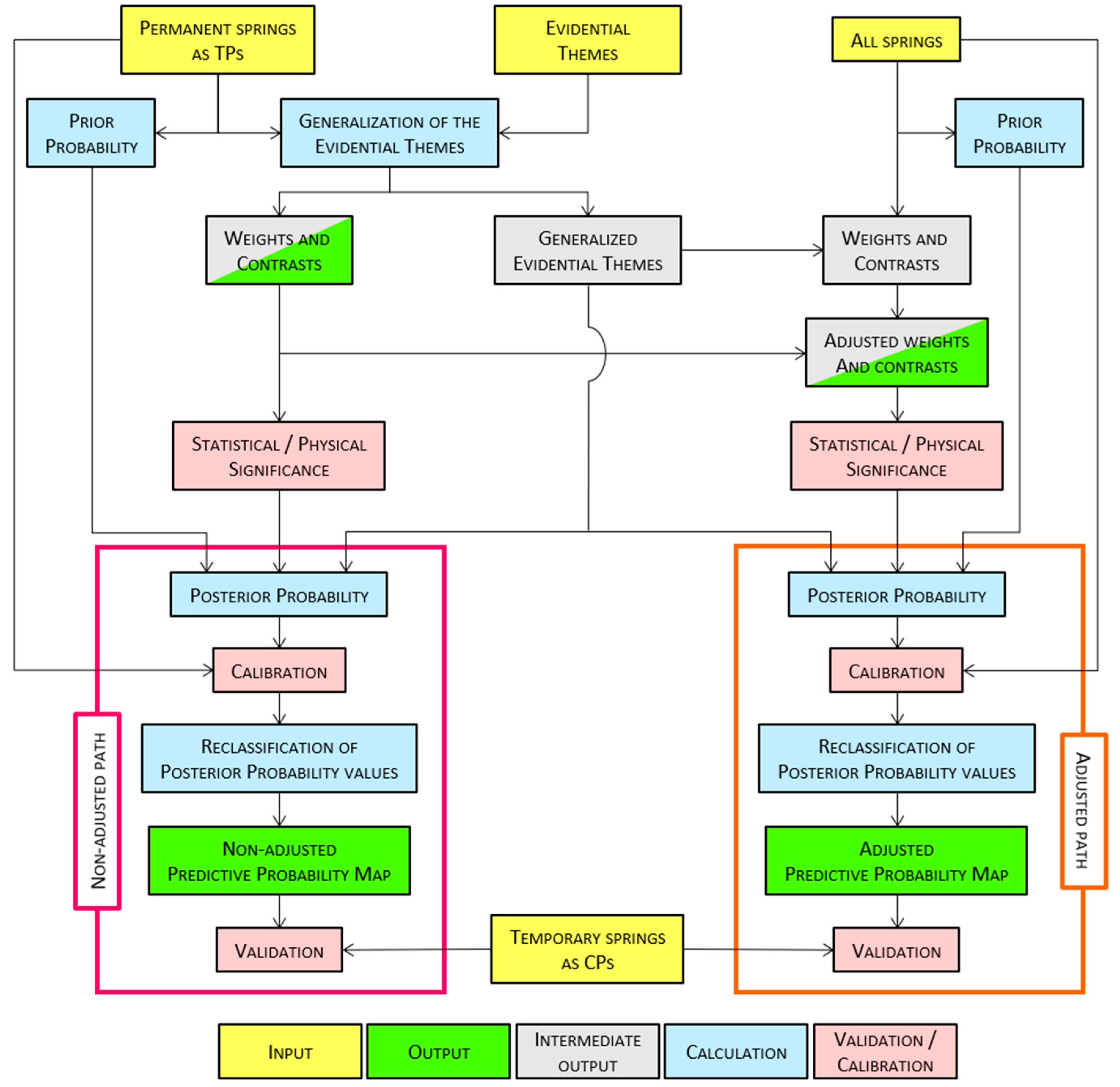
2.2. Workflow for the Application of the WofE Technique for Karst Springs

In this study, we introduced the application of the WofE technique to quantitatively evaluate the degree of spatial correlation between karst spring occurrences (as response variable) and geomorphological, geological, or physical factors (as evidential themes) influencing their presence in the study area.

We investigated two main questions through the WofE technique:

I

Q1—where is it possible to find karst springs?

II

Q2—where is it possible to identify the permanent karst springs?

The response variable, either training and control points (TPs or CPs, Table 1), was selected according to the question. Identified karst springs represent the response variable: in Q1 analysis, all the springs are assigned as TPs, whereas in Q2 analysis, the permanent springs are assigned as TPs and temporary springs are treated as CPs. The evidential themes are the same for the two questions and represent geological, geomorphological, and physical factors influencing the presence of karst springs (i.e., distribution of precipitation, terrain elevation, presence of faults, carbonate rocks, sinkholes, and sinking streams).

A common procedure for WofE application in hydrogeological studies [16,38] is used for answering Q1, as follows (Figure S1 in Supplementary Material):

• calculation of the prior probability;
• generalisation of the evidential themes, and evaluation of contrast C, weights W⁺ and W⁻;
• evaluation of the statistical and physical significance of the generalised evidential themes; and
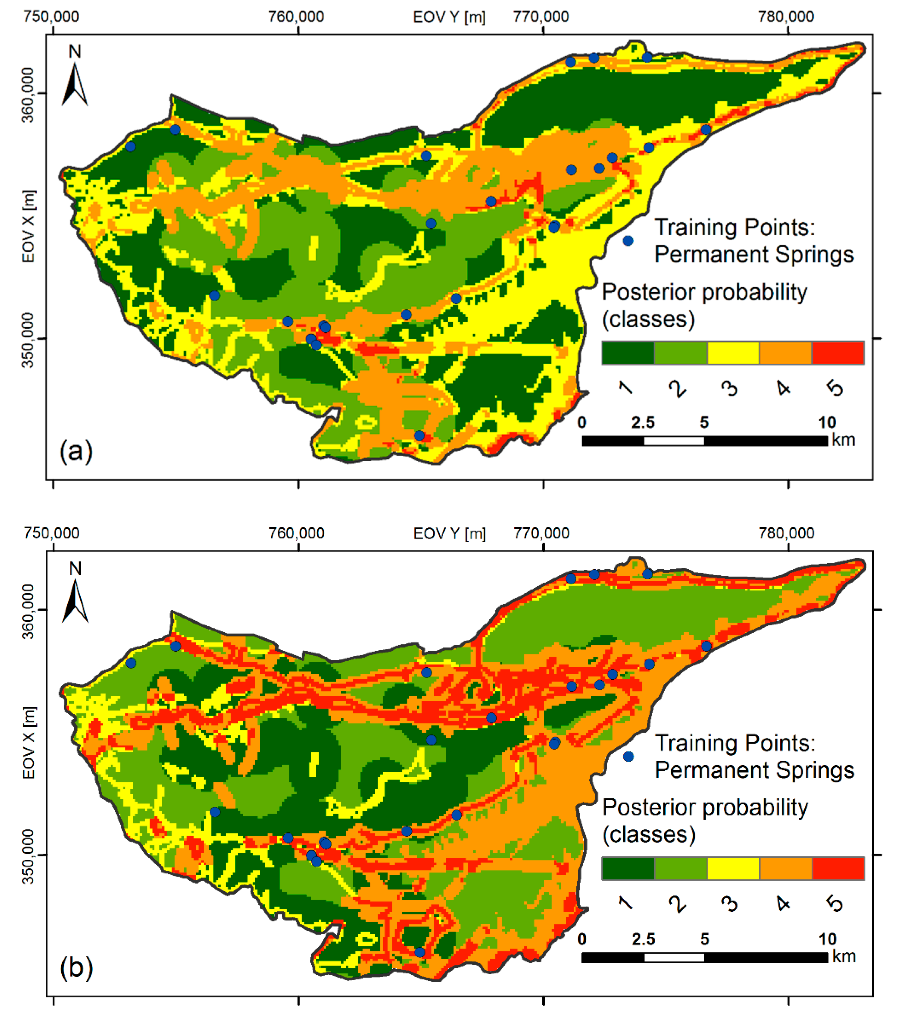
• creation of the posterior probability map.

Since all the identified karst springs are used as TPs, only one calibration analysis can be done. The obtained predictive (i.e., posterior) probability map represents the relative probability of identifying (i.e., individuating) karst springs.

We introduce a workflow in six steps for answering Q2, as follows (Figure 1):

• analysis using the permanent springs as TPs (calculation of the prior probability, generalisation of the evidential themes, evaluation of contrast C, weights W⁺ and W⁻, statistical and physical significance, and creation of the posterior probability map);
• analysis using all springs as TPs on the generalised evidential themes (evaluation of contrast C, weights W⁺ and W⁻, statistical and physical significance) and calculation of the prior probability;
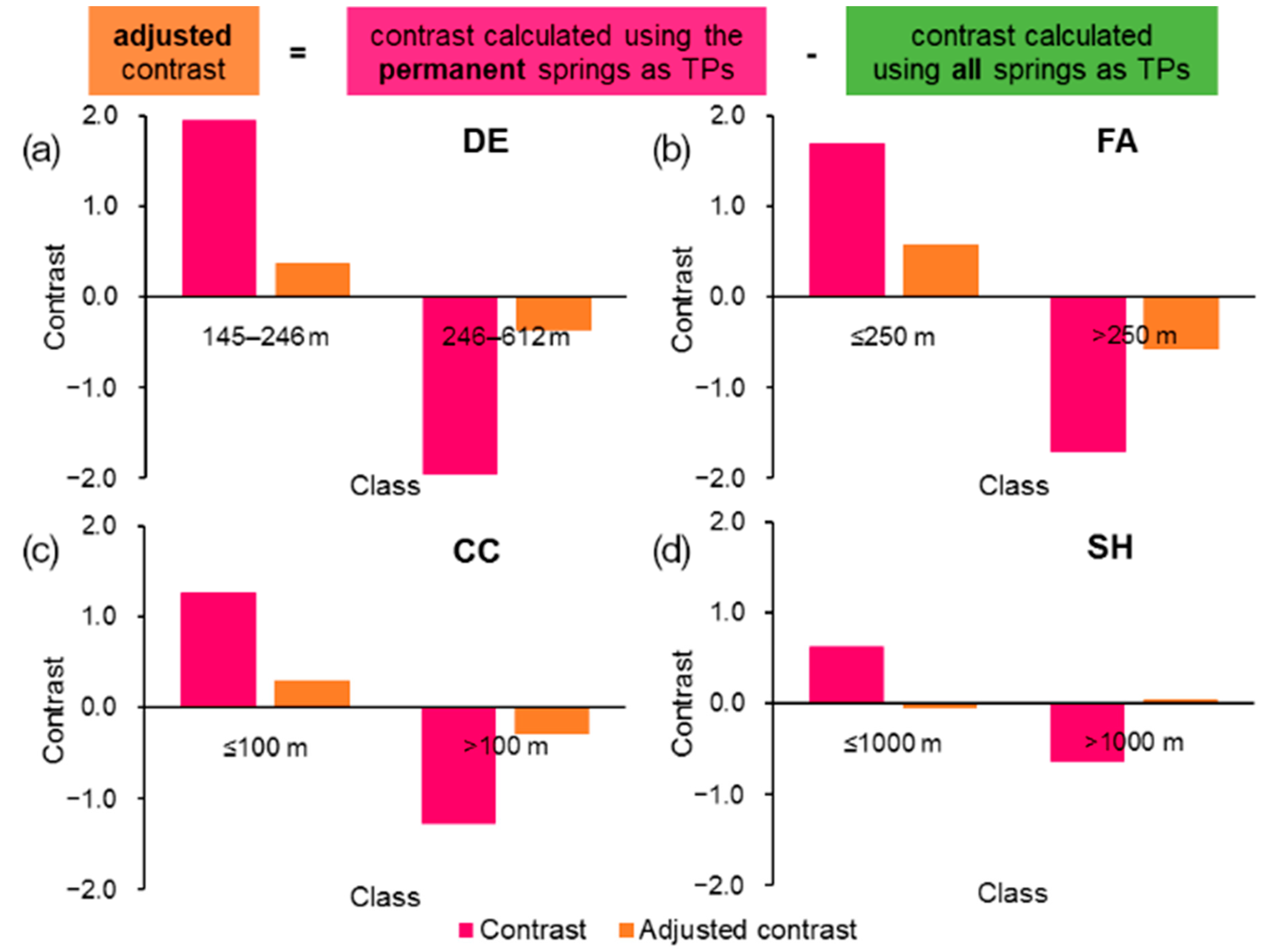
• calculation of the adjusted contrast and weights, by subtracting C, W⁺ and W⁻ calculated using all springs as TPs (step 2) from C, W⁺ and W⁻ calculated using the permanent springs as TPs (step 1);
• creation of the adjusted posterior probability map using: (i) the prior probability calculated using all springs and (ii) adjusted weights obtained from step 3;
• reclassification of the posterior probability values in 5 classes, using the geometrical interval classification method; and
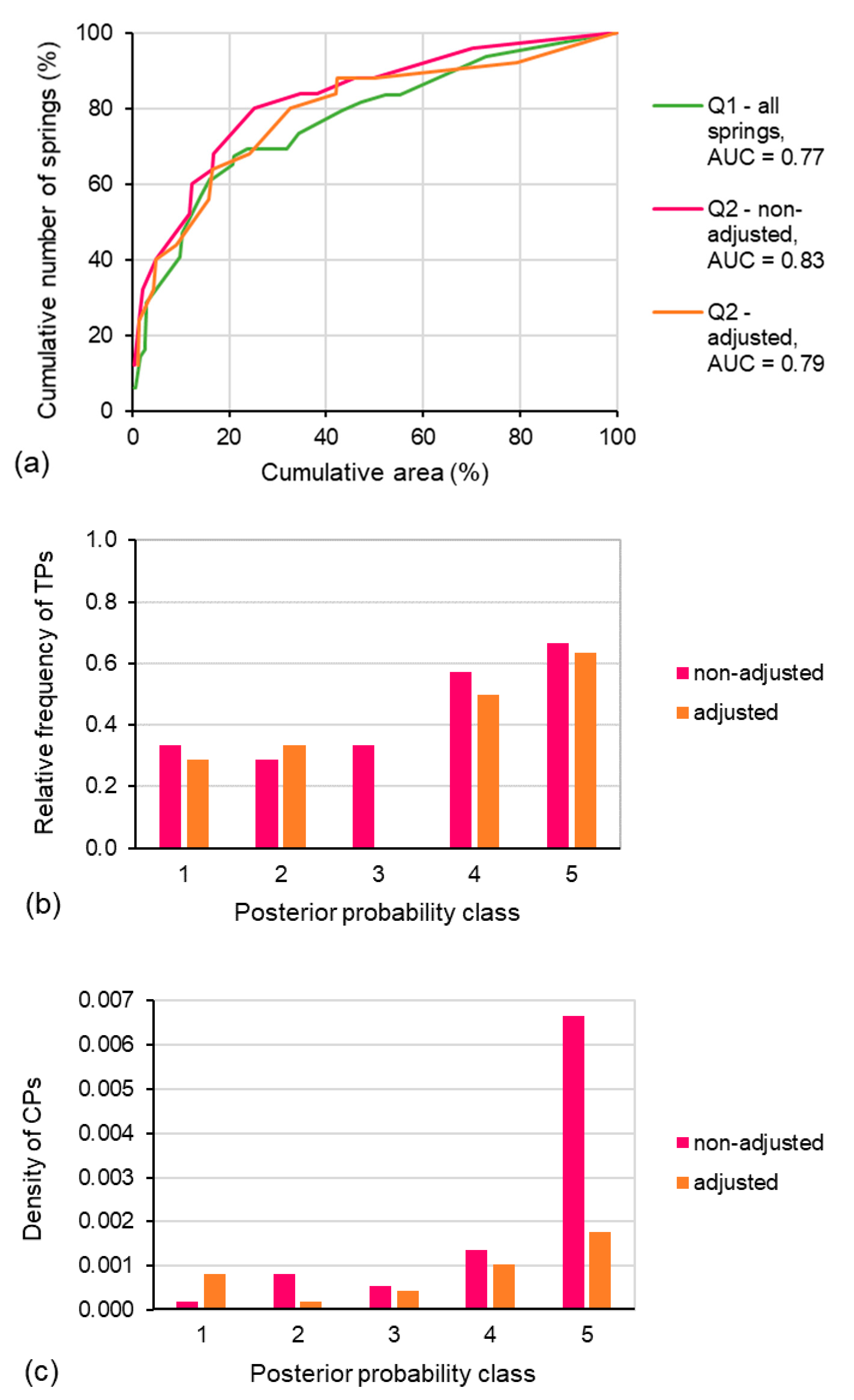
• comparison of the adjusted posterior probability map (step 4) with the posterior probability map, obtained using the standard WofE approach (step 1), and their derived reclassified maps, through calibration and validation techniques (Table 1). In this phase, we use the temporary springs, as CPs, for the validation of the adjusted map.

The adjusted posterior probability map displays the relative probability of identifying (i.e., individuating) permanent karst springs.

The demonstration of the proposed workflow by WofE technique was performed using the Arc Spatial Data Modeler geoprocessing tools [41]. A confidence value of 1.282, corresponding approximately to a 90% level of significance [23], was chosen as the minimum acceptable for considering an evidential theme class as statistically significant.

3. Application of the Proposed Workflow

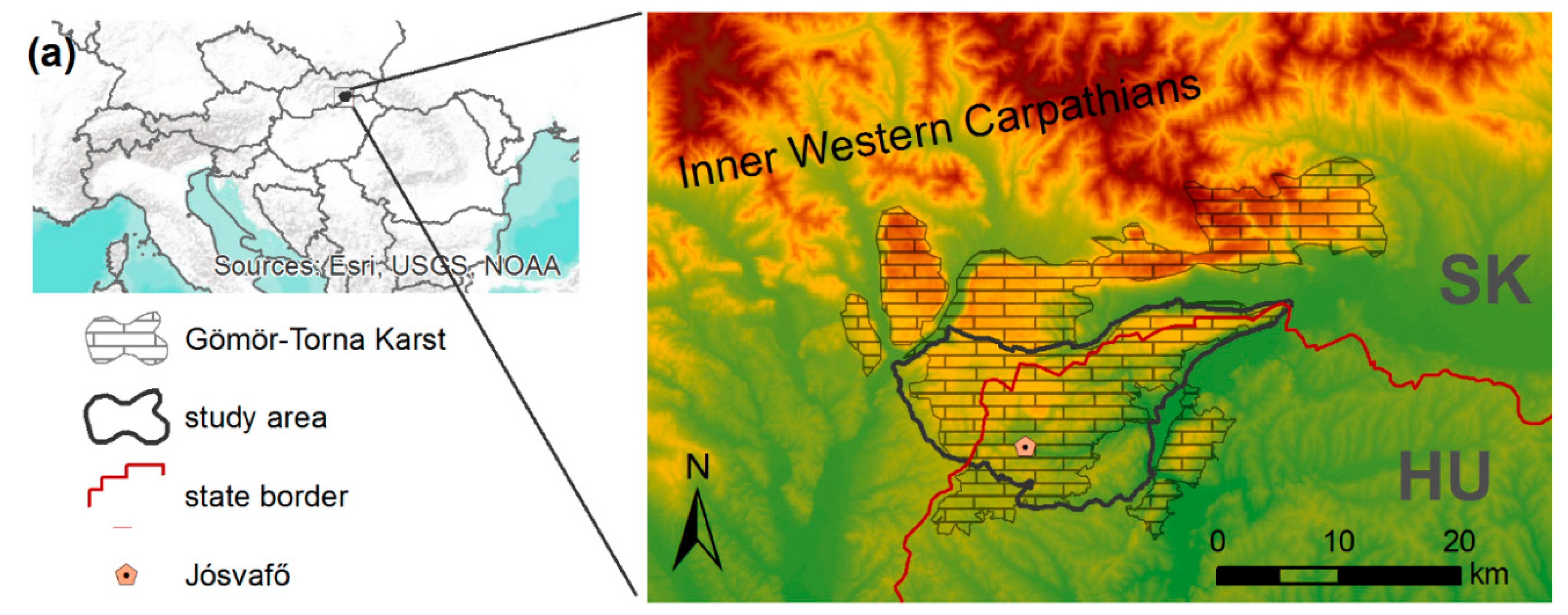
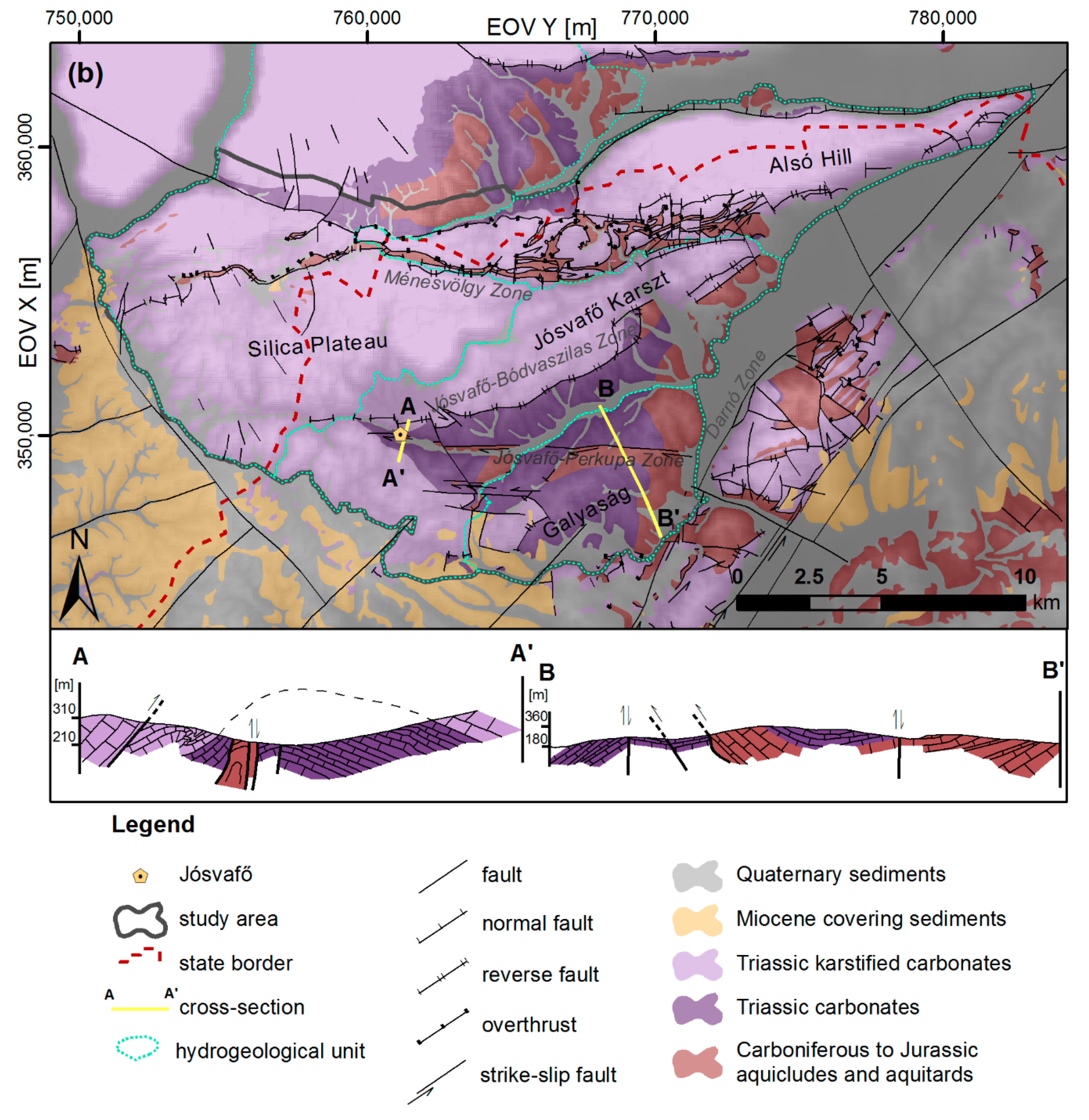
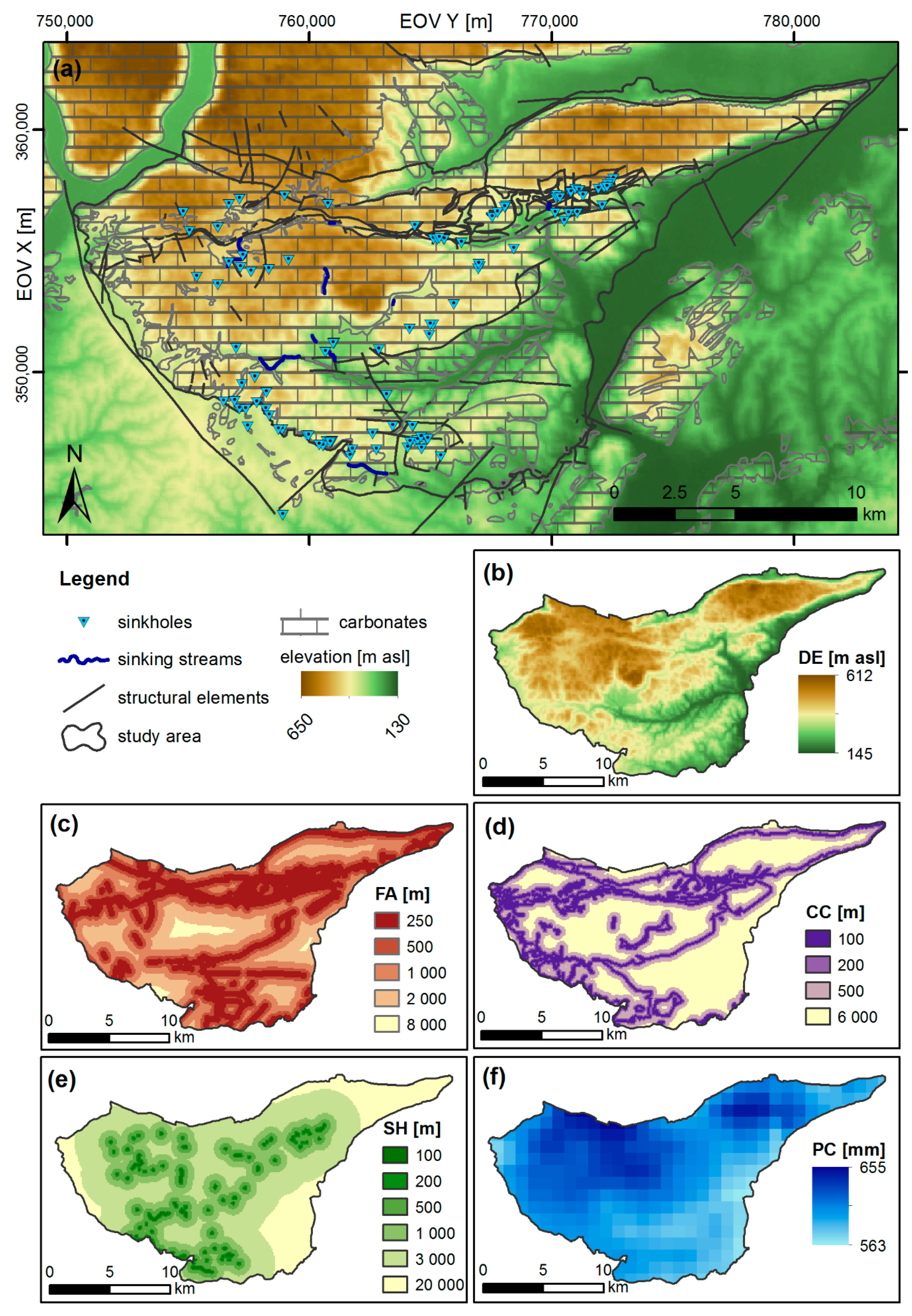
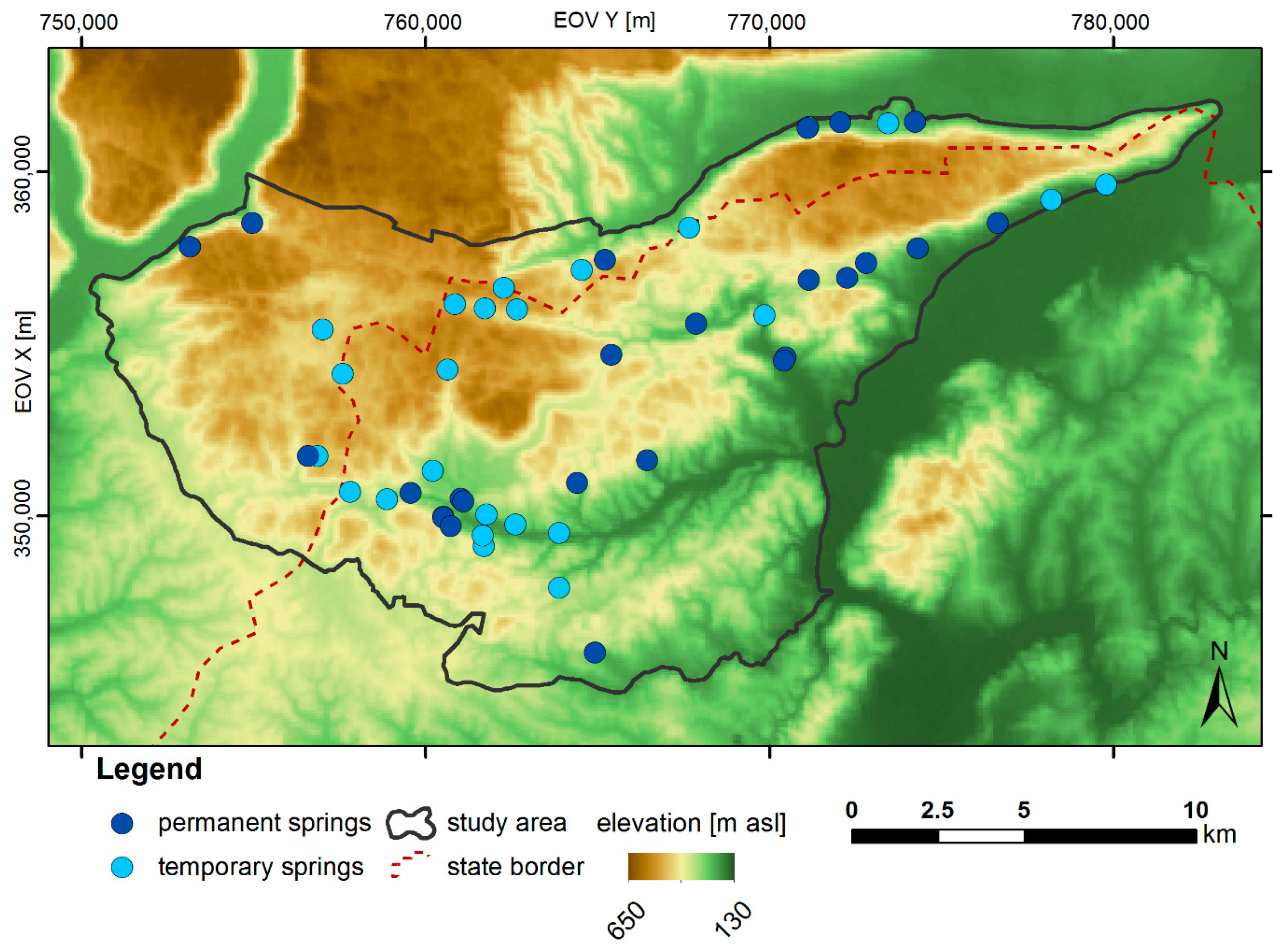
3.1. Geological and Hydrogeological Characterisation of the Study Area

The Gömör–Torna Karst lies on the border between Hungary and Slovakia, in Eastern Europe (Figure 2a). It is an unconfined karst area with extensive karstic landforms, such as caves (more than 700, up to 25 km length), dolines, canyon- and gorge-like valleys, sinkholes and karst springs [42,43]. The area can be characterized by mosaic-like topography: the doline-dotted karst plateaus are divided by tectonic-fluvial valleys [44], the elevation ranges between and 150 and 900 m a.s.l. Due to its complex natural heritage, the region is under the protection of the Aggtelek National Park (Hungary) and the Slovak Karst National Park (Slovakia). The Baradla–Domica Cave, along with other local caves, is part of the UNESCO World Heritage, since 1995.

The study area is part of the Aggtelek–Rudabánya Mountains in the Inner Western Carpathians [45]. It can be characterized by nappe structures, superponed by folded-imbricated structures. Above these, two horizontal deformation zones in east-western line of strike are detectable [45]. The main tectonic zones of the area are the Ménesvölgy Zone, the Jósvafő-Bódvaszilas Reverse Fault Zone, the Jósvafő-Perkupa Fault Zone and the Darnó Zone [46] (Figure 2b). The dominantly Middle (and Upper) Triassic carbonates of the Silica nappe form the main karstic aquifers of the area [45] (Figure 2b). Among the Triassic carbonates, large proportion is highly karstifiable, constituting an excellent aquifer, whilst being in complex tectonic relation with the aquitards: Permian evaporites, Triassic sandstones and marls [45] (see Figure 2b, legend colour symbol “Carboniferous to Jurassic aquicludes and aquitards”). The thickness of the karstified carbonates ranges typically from 400 to 1000 m [45]. Above the Triassic formations, Miocene covering sediments (such as continental, fluvial, and lacustrine sediments) and Quaternary sediments (such as gravels, various fluvial formations, and doline infillings—dominantly red clay—and slope sediments) are present. Fluvial formations are characterised by good hydraulic conductivity, whilst the doline infillings and slope sediments can be described as aquitards, with heterogeneous thickness [45]. The typical karst plateaus, with sinkholes and dolines, are separated by deep fluvial valleys [42], constituting smaller, connected, but nonetheless diverse hydrogeological units. Especially after precipitation or snowmelt, sinkholes transport water from the surface into the karst. According to the water balance equations in average 25–27% (min 9%, max 49%) of the precipitation infiltrates into the karst system through fissures and sinkholes [45]. The sinkholes of the area are diverse in terms of size, form, infilling, and activity, since they evolved in various position [42]. In the valleys sinkhole alignments and sinking streams can be found as well. Numerous karst springs are emerging on the area, ranging from the temporary, low discharging ones to the major permanent springs. In terms of discharge, they can be characterised by high variability: high-flow discharges may exceed baseflow discharge volumes by more than two orders of magnitude [45]. These springs provide drinking water for the inhabitants of the area on both sides of the countries’ border. The study area was delineated on the basis of the geological structures, geomorphological features, and the location of the springs, with an area of 281 km² (Figure 2). According to the structural and geomorphological elements, 4 main hydrogeological units can be differentiated on this area: Silica Plateau, Alsó Hill, Jósvafő Karst and Galyaság [47] (Figure 2b).

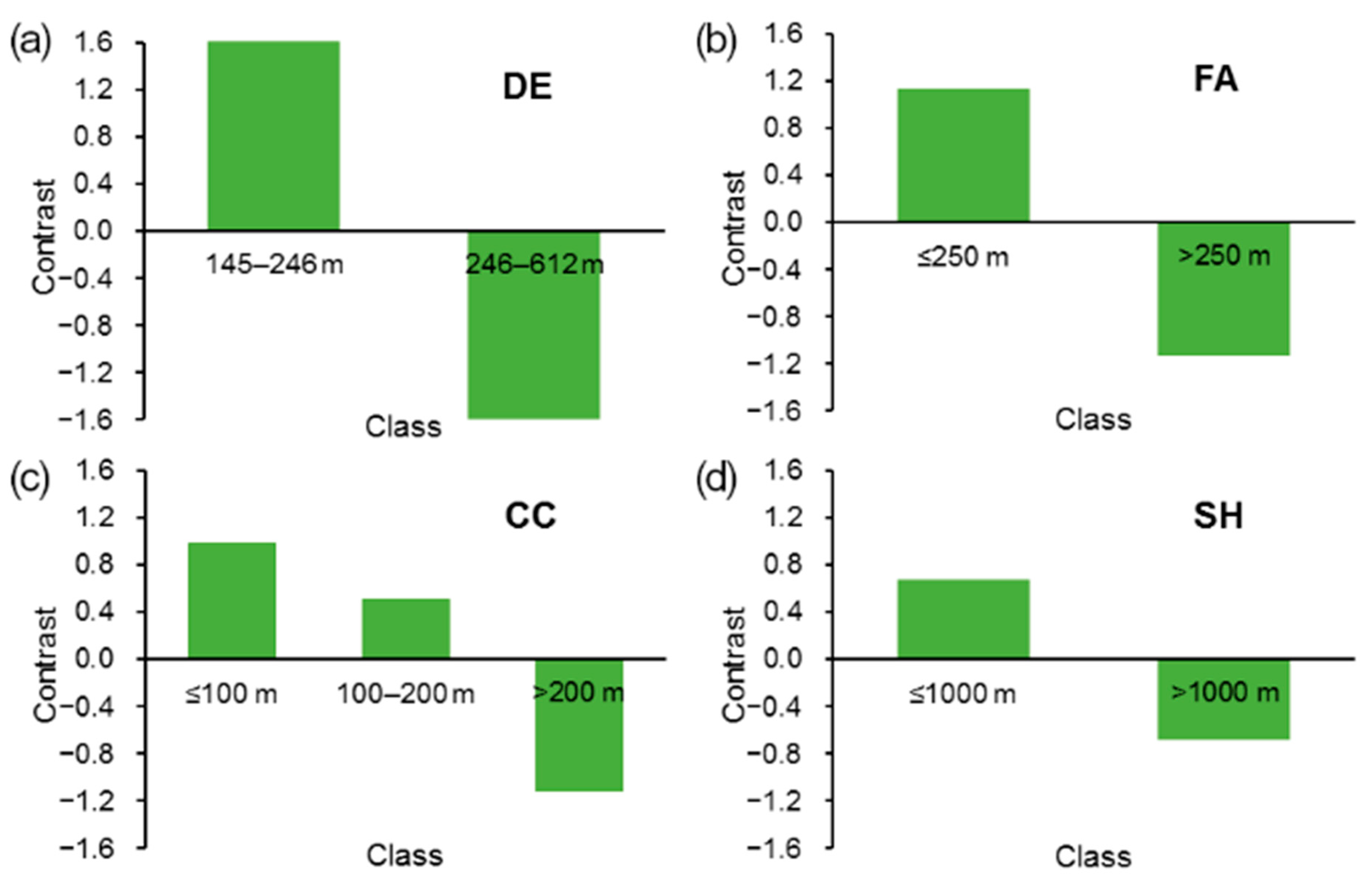
3.2. Evidential Themes

The evidential themes were selected on the basis of data availability and the following conceptual assumptions. The location and activity of springs are dependent on many factors: their elevations and the groundwater table depth; circumstances facilitating spring development, such as fractures, structural elements, and the contact zones between the carbonate aquifer and aquitards. Additionally, the recharge conditions are strongly influenced by the connection to concentrated infiltration points, and precipitation. According to the geomorphological, geological, and hydrogeological characteristics of the study area, five thematic maps were considered in the analysis as evidential themes: elevation (DE), distance to faults (FA), distance to the carbonate–non-carbonate rock contact (CC), distance to sinkholes and sinking streams (SH), and precipitation (PC).

The spatial distribution of these evidential themes was derived from multiple sources of information (

Table 2. Data sources and their uses.

Data	Use	Data Source
digital elevation model (SRTM, resolution of 3 arc-seconds)	evidential theme: DE	[48]
geological map (1:100,000)	evidential themes: FA and CC	[49]
sinkhole database (location)	evidential theme: SH	Cadastre of sinkholes (Aggtelek National Park)
modelled yearly average precipitation map (1000 m resolution)	evidential theme: PC	http://tinyurl.com/ClimateEU
spring database (location and activity: permanent or temporary)	response variables	[30]; Cadastre of springs (Aggtelek National Park)

, Figure 3a).

The elevation evidential theme was based on Shuttle Radar Topography Mission data with a resolution of 3 arc seconds (approximately 90 m), as a continuous type variable (Figure 3b). The distance to faults was evaluated as a categorical variable, based on buffer zones (with distances of 250, 500, 1000, and 2000 m), generated along the fracture zones of the geological map by Less et al. [49] (Figure 3c). The distance to the carbonate rock–non-carbonate rock contact was also generated by creating buffer zones based on the geological map. Along the contact zones, distances of 100, 200 and 500 m were used for this categorical type of evidential theme (Figure 3d). The distance to sinkholes and sinking streams categorical evidential theme was prepared on the basis of the sinkhole cadastre of the Aggtelek National Park, with buffer distances of 100, 200, 500, 1000, and 3000 m (Figure 3e). Lastly, the continuous type precipitation map was obtained on the basis of the yearly average precipitation map (1000 m resolution) of the 1961–1990 period. This base data was generated with the ClimateEU v4.63 software package, based on the method described by Wang, et al. [50], and downloaded from http://tinyurl.com/ClimateEU. In order to handle uneven data availability and data-scarce areas, the methodology uses adjustment of the precipitation data according to the elevation data [51] (Figure 3f).

These evidential themes, being the explanatory variables, were rasterised into 28,164 cells with a resolution of 100 m × 100 m for the study area.

3.3. Response Variables

Location of springs represents the response variables. The spring database contains 49 springs in the study area (Table 2). Among these, 25 are permanent springs, whilst 24 springs are temporary (Figure 4).

4. Results

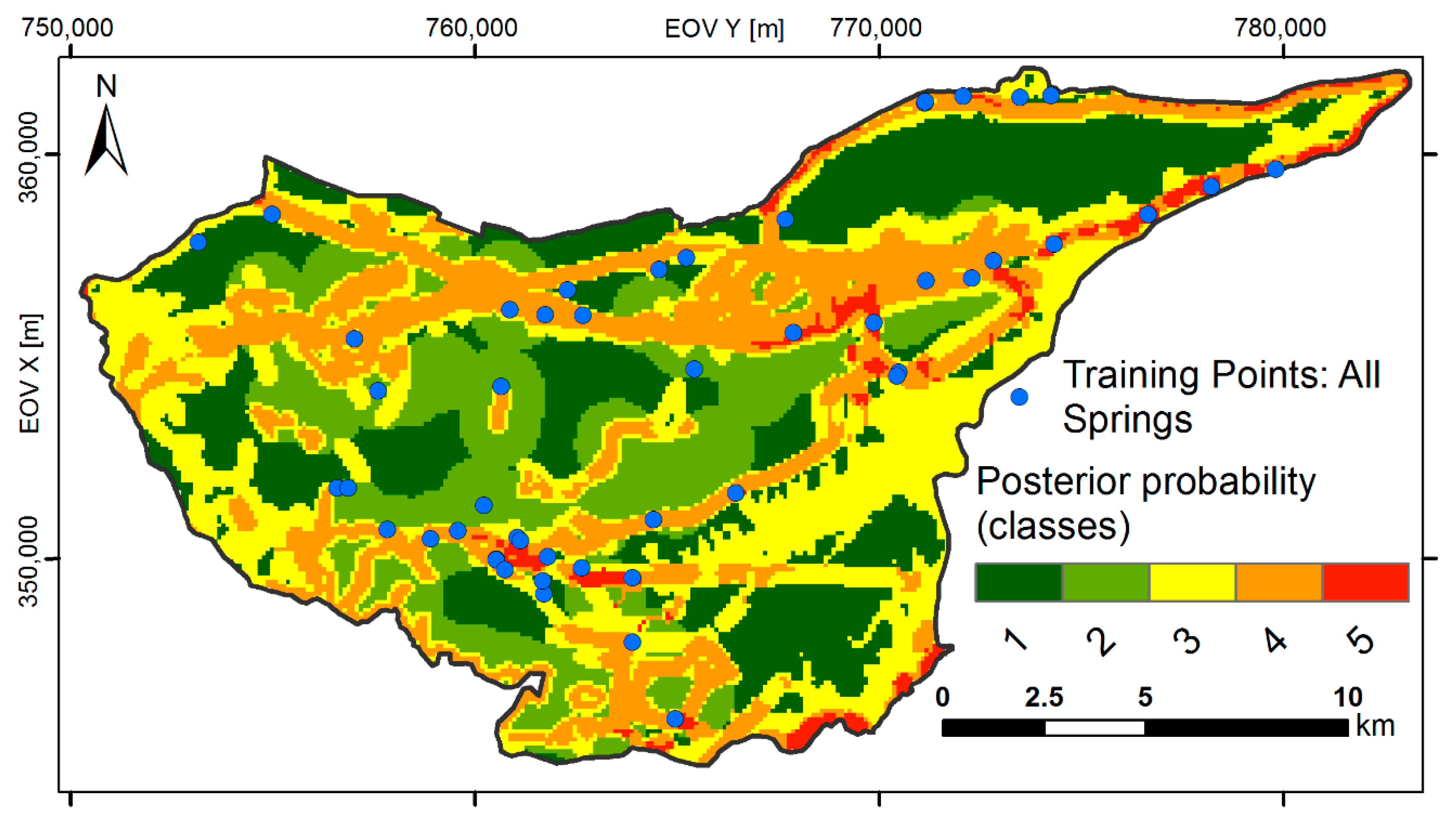
4.1. Location of Springs (Q1)

To answer Q1, first we evaluated statistically significant classes, their ranges and contrast values, for each evidential theme (Figure 5).

Elevation seems to play an important role in determining spring location: the probability of finding a spring is inversely related to elevation, and the greatest chance to find a spring is when the elevation is in its lowest range, between 145 and 246 m a.s.l. (Figure 5a). The analysis of contrasts shows a clear expected correlation between the position of springs and the main geological and structural elements (Figure 5b). The result highlights that the chance to find a spring is greatest when the distance from a fault or fracture is less than 250 m. There is an inverse correlation between spring position and the distance from the contact between carbonate and non-carbonate formations (Figure 5c), showing that the chance of finding a spring is greater when the distance is in the range between 0 and 100 m and very small when the distance is greater than 200 m. The analysis also shows that there is a high chance to have springs within 1000 m from sinkholes and sinking streams (Figure 5d). This result allows developing some hypotheses in terms of recharge that will be discussed in Section 5.

We did not report the histogram of contrast for the precipitation evidential theme because the variable was not shown to be statistically significant. This result could be related to several factors: (i) the precipitation map is highly correlated with the elevation map; (ii) the resolution of the precipitation map is too rough with respect to the extension of the study area and the distribution of karst springs; (iii) the amount of precipitation varies in a small range within the study area. Nevertheless, considering that these reasons are site-specific, the precipitation may be discriminant on other study areas.

The computation of the predictive probability map is based on the combination of the four statistically and physically significant evidential themes: DE, FA, CC, and SH. This map represents the relative probability of identifying springs in the study area. From this result, we prepared the posterior probability map by reclassification into five classes, with the probability increasing from class 1 to class 5 (Figure 6).

As represented in Figure 6, the zones that are more likely to contain a karst spring cover small portions of the study area indicated by red and orange. They are distributed along the southern and southeastern borders and affect some parts of the central and north-eastern sectors. The areal extent of areas shown by orange are greater compared to those in red, which have the greatest probability.

4.2. Location of Permanent Springs (Q2)

The resulting classes with their ranges were obtained from the generalisation of the evidential themes using the permanent springs as TPs. We represent their contrast and the adjusted contrast values in Figure 7. The adjusted contrasts (and weights) are used for identifying the correct relationship between the location of the permanent springs and the evidential themes, as this relation may be biased due to the non-random distribution of the known permanent springs (i.e., the location of some springs in the study area may still be undiscovered).

The analysis of adjusted contrasts shows that three of the four evidential themes (distance from the contact between carbonate and non-carbonate formation, distance from main faults and fractures, elevation) maintain the same type of correlation with the position of the springs resulting for all the springs. For these evidential themes, the difference is given by the decrease of the absolute value of contrasts.

The distance to sinkholes and sinking streams is the only evidential theme that shows a correlation that is the opposite of the total springs case. The result is a direct correlation between the chances to have a permanent spring with the increase of the distance from a sinkhole. This result is quite interesting because it is consistent with a common relationship between location of direct recharge zones and spring regime, which we discuss in Section 5.

The predictive probability maps were generated by combining the generalised evidential themes using the non-adjusted contrast and adjusted contrast values. This model represents the relative probability of identifying permanent springs in the study area. The posterior probability maps are reclassified into five classes, with the probability increasing from class 1 to class 5 (Figure 8).

The reclassified posterior probability map produced by using the non-adjusted contrasts (Figure 8a) revealed a spatial distribution of the probability classes remarkably similar to that obtained within the map presented in Figure 6 and described above. This means that the importance of each individual evidential theme in predicting the presence of a generic karst spring has remained the same also in predicting the presence of permanent springs.

After adjusting the contrast values, the role of each evidential theme has changed, resulting in a different distribution of the probability classes as shown in the map in Figure 8b. In this map, both classes 4 and 5, which reflect the high and the extremely high probability of finding a permanent spring, respectively, are much more widespread and cover larger areas. On the other hand, class 3 has a dramatic reduction of extension, with few zones found in the most western sector.

4.3. Validation

The efficacy of the posterior probability maps has been evaluated by calculating the Area Under the Curve (AUC) values. AUC values are equal to 77%, 83%, and 79% for the ‘total’, ‘non-adjusted’, and ‘adjusted’ predictive probability maps, respectively (Figure 9a). These results show the high quality of the maps.

The predictive power of the reclassified posterior probability maps has been assessed by applying the following validation procedures: the relative frequency of TPs, expressed as the ratio between the number of TPs and the total number of springs (TPs + CPs) within each posterior probability class, and the density of CPs, expressed as the ratio between the number of CPs and the total number of cells within each posterior probability class. These procedures have not been applied to the reclassified response theme obtained using all springs as TPs (Figure 6), since there are no CPs (Section 2.2). In the ‘non-adjusted’ and ‘adjusted’ cases, the histograms show that, in general, the frequency of the training set (i.e., permanent springs) increases from posterior probability class 1 to class 5, as expected [38]. Nevertheless, both histograms reveal some anomalies (Figure 9b). Class 1 of the ‘non-adjusted’ case (i.e., pink columns) is characterised by a frequency of TPs greater than that of class 2 and, like class 3, showing some bias in the lowest posterior probability classes. The ‘adjusted’ case shows a more clear and accurate monotonic increase from class 1 to class 5, even if it has a null value for class 3. This clear flaw does not significantly affect the excellent quality of the results, because it is related to the small area covered by class 3 in this case. This situation decreases the overall chance to have a TP (or even a CP) within a class and gives to the frequency value a low reliability.

The histograms representing the density of CPs in each posterior probability class highlights quite different results for the ‘adjusted’ and ‘non-adjusted’ cases. The ‘non-adjusted’ case performs very poorly, showing an increase in the density of CPs from class 1 to class 5 (Figure 9c). In fact, the expectancy is a decreasing of the density of CPs from class 1 to class 5 [38]. Moreover, the spatial density of CPs is much greater in class 5 than in all other classes. The density value of class 5 is more than five times greater than in all other classes and more than 20 times greater than the value in class 1. Class 1 has the lowest density value of all classes. Even if the general trend in the ‘adjusted’ case is not completely consistent with the expectation, there is a significant improvement in the results. Class 5 is still the one with the greatest CP density value, but it is less than two times bigger than the value of class 1. The class 1 density value is higher than the ones for class 2 and class 3 and just a little bit lower than for class 4.

5. Discussion

The analyses show that elevation seems to play a key role in determining the location of the springs. This result can be partially related to the fact that within the higher elevation range, the potential aquifers contained in the permeable formations could be not thick enough to contain enough volume of water storage necessary to create permanent or temporary springs. In addition, this result is in accordance with the gravity-driven flow forces prevailing not only in siliciclastic, but also in karst areas [52].

Faults and fractures can form both conduits and barriers in groundwater flow, so their actual hydraulic function is dependent on various factors [53,54]. The study area is characterised by a complex structural setting [45,46,55]. The previous findings, that the correlation found between spring position and the main faults and fractures in the area is inverse, seem to indicate that these lineaments also have an important hydrogeological influence by acting more as barriers (by creating contacts between permeable and less permeable formations) than as areas of increased recharge.

Karst aquifers present a characteristic duality in infiltration processes (diffuse type and, connected to sinkholes, concentrate type). The duality appears in the flow components as well, as slow matrix flow and quick conduit flow. As a result, the hydrograph of karst springs consists of baseflow and quickflow components [56,57,58,59,60]. The high chance of having springs within 1000 m from sinkholes and sinking streams (Figure 5d) can be viewed within the general recharge process of springs. In terms of recharge, this result shows that many springs should have a fast recharge component that it is not necessarily the only one but should have a significant role in the hydrogeological regime of many springs. In particular, the proximity of springs to direct recharge can affect the permanent or transient regime of spring discharge in correlation with the results of spring hydrograph analyses [61]. In general, when the recharge zone is close to the spring, there is a high chance that it will show a transient regime; on the other hand, those springs for which the recharge zone is distant tend to maintain a non-zero discharge all through the year [12]. This matter is further discussed below for the analyses of the distinction between temporary and permanent springs.

The distribution of areas with a high probability of finding a spring is the result of the presence of geological and structural elements favourable for their formation. These ideal conditions occur at low altitudes (145–246 m a.s.l.) and in proximity to both structural lineaments (≤250 m) and contact zones between permeable and less-permeable formations (≤200 m). As shown by the analysis of the contrast values, the most conditioning variable is represented by the elevation, which plays a key role in controlling the spatial distribution of the probability within the area of interest. In fact, the sectors with exceptionally low and low probabilities correspond to those characterised by high elevation values. As the elevation decreases, the probability of finding a karst spring increases, reaching heightened values in areas where the influence exerted by the elevation is combined with the effect due to the proximity to faults and/or contact zones between weight adjustment is performed.

When observing the areas with a high probability of finding a permanent spring (class 5 in Figure 8b), their distribution is a consequence of the significant influence exerted by the proximity to the main structural lineaments (≤250 m), which proved to be the most impacting variable in discriminating among areas with low and high probability of containing a permanent spring. Although the distance to sinkholes and sinking streams highlighted a different behaviour in influencing the presence of a permanent spring, it provided very low contrast values, reflecting a moderate importance of this variable in conditioning the distribution of the probability classes. On the other hand, elevation and the distance to the carbonate and non-carbonate rock contact were still found to have a significant control on the presence of permanent springs by increasing the probability in areas located at low altitudes (145–246 m a.s.l.) and very close to contact zones between permeable and less permeable formations (≤100 m). These areas are identified by probability classes 3 and 4 in Figure 8b.

6. Summary and Conclusions

In this study, the WofE technique has proven to be robust in predicting and mapping the occurrence of karst springs as well as permanent springs on the basis of the proposed workflow. Its effectiveness has been confirmed by the results obtained from the application of the AUC technique and the validation procedures, which highlighted the good degree of accuracy of the posterior probability maps in correctly classifying the occurrence of both temporary and permanent karst springs.

The study answered two questions, about the location of springs (Q1) and of the temporary and permanent springs (Q2), respectively, in an unconfined karst area; future research might extend the explanations of factors influencing groundwater vulnerability. The comparison of the patterns of the Q1 and Q2 maps shows major similarities. From this we can assume that most of the parameters are similarly affecting both the permanent and temporary springs. However, a significant difference can be detected in the case of the effect of the sinkholes and sinking streams: it is proven that the vicinity of sinkholes or sinking streams predicts the temporary springs more accurately.

The produced predictive maps stand as an essential tool for implementing water resource management and protection measures. In particular, the delineation of areas holding potential karstic springs, and especially permanent springs, can be useful for planners and decision-makers to identify locations at which to enhance resource explorations and to address water availability problems. The proposed statistical approach can especially be helpful in less broadly studied, data-scarce areas, to effectively delineate the zones with favourable characteristics for not just spring occurrences, but appropriate well locations as well.

In addition to the predictive outputs, the WofE technique was used to gain a deeper comprehension of the geological and structural conditions favourable for the formation of the springs in a quantitative manner. In agreement with earlier studies (e.g., [21,62]), distance to tectonic structures and elevation were found to be the most influencing variables controlling the occurrence of karst springs and permanent springs within the study area.

In the karst area of the Transdanubian Central Range, Mádl-Szőnyi and Tóth [52] demonstrated systematic correlation of physico-chemical spring parameters (discharge volume, temperature, and chloride content) with their elevation of discharge. On the basis of these parameters, the springs can be grouped, being related to local, intermediate and regional flow systems. Stable discharge volume is a characteristic of intermediate and regional flow, whilst springs of the local flow systems show high variability of discharge volume, or even temporarily dry up. The analysis of several springs of the Gömör–Torna Karst also revealed that the discharge volume and the temperature increases, whilst the variability of discharge volume decreases, with the elevation [29,61]. All these findings highlight the importance of the concept of groundwater flow systems whilst addressing water management issues.

The presented workflow has the potential for the application in other unconfined karst areas and widening the circle of examined questions. In further studies, besides spring temporality, other spring properties can be studied as response variables, such as indicators of spring vulnerability. Thus, the method would provide an aim to water management regarding fresh karst water quantity and quality.

References

1. Ford, D.; Williams, P.D. Karst Hydrogeology and Geomorphology; Wiley: Hoboken, NJ, USA, 2007. [Google Scholar]
2. Goldscheider, N.; Drew, D. Methods in Karst Hydrogeology: IAH: International Contributions to Hydrogeology, 26; CRC Press: Boca Raton, FL, USA, 2007. [Google Scholar]
3. Zwahlen, F. Vulnerability and Risk Mapping for the Protection of Carbonate (Karst) Aquifers, Final Report (COST Action 620). European Commission, Directorate-General XII Science; Office for Official Publications of the European Communities: Brussels, Belgium, 2004.
4. Gleick, P.H. Climate change, hydrology, and water resources. Rev. Geophys. 1989, 27, 329–344. [Google Scholar] [CrossRef]
5. Butscher, C.; Huggenberger, P. Modeling the Temporal Variability of Karst Groundwater Vulnerability, with Implications for Climate Change. Environ. Sci. Technol. 2009, 43, 1665–1669. [Google Scholar] [CrossRef] [Green Version]
6. Taylor, R.G.; Scanlon, B.; Döll, P.; Rodell, M.; Van Beek, R.; Wada, Y.; Longuevergne, L.; Leblanc, M.; Famiglietti, J.S.; Edmunds, M. Ground water and climate change. Nat. Clim. Chang. 2013, 3, 322–329. [Google Scholar] [CrossRef] [Green Version]
7. Green, T.R. Linking climate change and groundwater. In Integrated Groundwater Management; Springer: Cham, Switzerland, 2016; pp. 97–141. [Google Scholar]
8. Toth, J. Groundwater discharge: A common generator of diverse geologic and morphologic phenomena. Hydrol. Sci. J. 1971, 16, 7–24. [Google Scholar] [CrossRef]
9. Engelen, G.B.; Kloosterman, F.H. Hydrological Systems Analysis: Methods and Applications; Springer Science & Business Media: Berlin, Germany, 2012; Volume 20. [Google Scholar]
10. Goldscheider, N. Hydrogeology and Vulnerability of Karst Systems: Examples from the Northern Alps and the Swabian Alb. Ph.D. Thesis, Karlsruhe University, Karlsruhe, Germany, 2002. [Google Scholar]
11. Tóth, J. Springs seen and interpreted in the context of groundwater flow-systems. In Proceedings of the GSA Annual Meeting, Portland, OR, USA, 18–21 October 2009. [Google Scholar]
12. Kresic, N.; Stevanovic, Z. Groundwater Hydrology of Springs: Engineering, Theory. In Management, and Sustainability; Elsevier: Amsterdam, The Netherlands, 2010. [Google Scholar]
13. Iván, V.; Mádl-Szőnyi, J. State of the art of karst vulnerability assessment: Overview, evaluation and outlook. Environ. Earth Sci. 2017, 76, 112. [Google Scholar] [CrossRef]
14. Stevanović, Z. Karst Aquifers—Characterization and Engineering; Stevanović, Z., Ed.; Springer International Publishing: Cham, Switzerland, 2015; p. 692. [Google Scholar]
15. Bonacci, O.; Terzić, J.; Roje-Bonacci, T.; Frangen, T. An Intermittent Karst River: The Case of the Čikola River (Dinaric Karst, Croatia). Water 2019, 11, 2415. [Google Scholar] [CrossRef] [Green Version]
16. Sorichetta, A.; Masetti, M.; Ballabio, C.; Sterlacchini, S. Aquifer nitrate vulnerability assessment using positive and negative weights of evidence methods, Milan, Italy. Comput. Geosci. Uk 2012, 48, 199–210. [Google Scholar] [CrossRef]
17. Bonham-Carter, G.F. Geographic Information Systems for Geoscientists-Modeling with GIS. Comput. Methods Geosci. 1994, 13, 398. [Google Scholar]
18. Raines, G.L. Evaluation of weights of evidence to predict epithermal-gold deposits in the Great Basin of the Western United States. Nat. Resour. Res. 1999, 8, 257–276. [Google Scholar] [CrossRef]
19. Sterlacchini, S.; Ballabio, C.; Blahut, J.; Masetti, M.; Sorichetta, A. Spatial agreement of predicted patterns in landslide susceptibility maps. Geomorphology 2011, 125, 51–61. [Google Scholar] [CrossRef]
20. Lee, S.; Kim, Y.-S.; Oh, H.-J. Application of a weights-of-evidence method and GIS to regional groundwater productivity potential mapping. J. Environ. Manag. 2012, 96, 91–105. [Google Scholar] [CrossRef] [PubMed]
21. Corsini, A.; Cervi, F.; Ronchetti, F. Weight of evidence and artificial neural networks for potential groundwater spring mapping: An application to the Mt. Modino area (Northern Apennines, Italy). Geomorphology 2009, 111, 79–87. [Google Scholar] [CrossRef]
22. Cervi, F.; Blöschl, G.; Corsini, A.; Borgatti, L.; Montanari, A. Perennial springs provide information to predict low flows in mountain basins. Hydrol. Sci. J. 2017, 62, 2469–2481. [Google Scholar] [CrossRef]
23. Arthur, J.D.; Wood, H.A.R.; Baker, A.E.; Cichon, J.R.; Raines, G.L. Development and implementation of a Bayesian-based aquifer vulnerability assessment in Florida. Nat. Resour. Res. 2007, 16, 93–107. [Google Scholar] [CrossRef]
24. Pollicino, L.C.; Masetti, M.; Stevenazzi, S.; Colombo, L.; Alberti, L. Spatial Statistical Assessment of Groundwater PCE (Tetrachloroethylene) Diffuse Contamination in Urban Areas. Water 2019, 11, 1211. [Google Scholar] [CrossRef] [Green Version]
25. Kessler, H. Az aggteleki barlangrendszer hidrográfiája [The hydrology of the Aggtelek Cave System]. Földr. Közl 1938, 66, 1–30. [Google Scholar]
26. Jakucs, L. Vízföldtani megfigyelések a Gömöri-karszton [Hydrogeological observations on the Gömör Karst]. Földt. Közl 1951, 81, 442–445. [Google Scholar]
27. Izápy, G.; Maucha, L. Az Aggteleki-hegység karszthidrológiai vizsgálata a Jósvafői kutató állomáson. In Karsztvízkutatás Magyarországon Ia. kötet. Felszín alatti vizeink kutatása, feltárása, hasznosítása és védelme. Szemelvények a kutatás és oktatás intézményeinek munkáiból; VITUKI: Budapest, Hungary, 2004. [Google Scholar]
28. Gruber, P. A Baradla–Domica-barlangrendszer hidrológiai kutatásának eredményei [Summary of the Hydrologycal Research of the Baradla–Domica Cave System]. Karsztfejlődés [Karst Development] 2016, 21, 187–201. [Google Scholar] [CrossRef]
29. Iván, V.; Mádl-Szőnyi, J. Vulnerability assessment and its validation: The Gömör-Torna Karst, Hungary and Slovakia. Geol. Soc. Lond. Spec. Publ. 2017, 466. [Google Scholar] [CrossRef]
30. Maucha, L. Az Aggteleki-hegység karszthidrológiai kutatási eredményei és zavartalan hidrológiai adatsorai 1958–1993 [Results and undisturbed data of karst hydrological researches on Aggtelek Hills 1958–1993 (in Hungarian)]. VITUKI Rt. Hidrológiai kiadványa 1998, 414. [Google Scholar]
31. Masetti, M.; Poli, S.; Sterlacchini, S.; Beretta, G.P.; Facchi, A. Spatial and statistical assessment of factors influencing nitrate contamination in groundwater. J. Environ. Manag. 2008, 86, 272–281. [Google Scholar] [CrossRef] [PubMed]
32. Arthur, J.D.; Baker, A.E.; Cichon, J.R.; Wood, A.R.; Rudin, A. Florida Aquifer Vulnerability Assessment (FAVA): Contamination potential of Florida’s principal aquifer systems. In Report Submitted to the Division of Water Resource Management, Florida Department of Environmental Protection. Tallahassee: Division of Resource Assessment and Management; Florida Geological Survey: Tallahassee, FL, USA, 2005. [Google Scholar]
33. Sorichetta, A.; Ballabio, C.; Masetti, M.; Robinson Jr, G.R.; Sterlacchini, S. A Comparison of Data-Driven Groundwater Vulnerability Assessment Methods. Groundwater 2013, 51, 866–879. [Google Scholar] [CrossRef] [PubMed]
34. Albinet, M.; Margat, J. Cartographie de la vulnerabilité à la pollution des nappes d’eau souterraines. Bull. BRGM 1970, 2ème série 3, 13–22. [Google Scholar]
35. Coolbaugh, M.F.; Raines, G.L.; Zehner, R.E. Assessment of exploration bias in data-driven predictive models and the estimation of undiscovered resources. Nat. Resour. Res. 2007, 16, 199–207. [Google Scholar] [CrossRef]
36. Sorichetta, A.; Robinson, G.R., Jr. Groundwater vulnerability assessment using positive and negative Weights-of-Evidence methods to correct for sampling bias. In Proceedings of the Flowpath 2012, Bologna, Italy, June 20–22 2012. [Google Scholar]
37. Focazio, M.J. Assessing Ground-water Vulnerability to Contamination: Providing Scientifically Defensible Information for Decision Makers; US Dept. of the Interior, US Geological Survey: Reston, VA, USA, 2002; Volume 1224.
38. Sorichetta, A.; Masetti, M.; Ballabio, C.; Sterlacchini, S.; Beretta, G.P. Reliability of groundwater vulnerability maps obtained through statistical methods. J. Environ. Manag. 2011, 92, 1215–1224. [Google Scholar] [CrossRef] [PubMed]
39. Cowan, N. The magical number 4 in short-term memory: A reconsideration of mental storage capacity. Behav. Brain Sci. 2001, 24, 87–114. [Google Scholar] [CrossRef] [PubMed] [Green Version]
40. Chung, C.-J.F.; Fabbri, A.G. Probabilistic prediction models for landslide hazard mapping. Photogramm. Eng. Remote Sens. 1999, 65, 1389–1399. [Google Scholar]
41. Sawatzky, D.; Raines, G.; Bonham-Carter, G.; Looney, C. Spatial Data Modeller (SDM): ArcMAP 9.3 Geoprocessing Tools for Spatial Data Modelling Using Weights of Evidence, Logistic Regression, Fuzzy Logic and Neural Networks. 2009. Available online: http://www.ige.unicamp.br/sdm/ (accessed on 5 June 2019).
42. Zámbó, L. Az Aggteleki-karszt felszínalaktani jellemzése. Geomorphological characterization of the Aggtelek Karst. Földrajzi értesitö 1998, 47, 359–378. [Google Scholar]
43. Gessert, A. Geomorphology of the Slovak Karst (Eastern Part). J. Maps 2016, 12, 285–288. [Google Scholar] [CrossRef]
44. Telbisz, T.; Gruber, P.; Mari, L.; Kőszegi, M.; Bottlik, Z.; Standovár, T. Geological Heritage, Geotourism and Local Development in Aggtelek National Park (NE Hungary). Geoheritage 2020, 12, 5. [Google Scholar] [CrossRef] [Green Version]
45. Szentpétery, I.; Less, G. Az Aggtelek–Rudabányai-hegység Földtana. Magyarázó az Aggtelek–Rudabányai-Hegység 1988-ban Megjelent 1: 25 000 Méretarányú Fedetlen Földtani Térképéhez.(Geology of the Aggtelek–Rudabánya Hills. Explanatory Book to the Pre-Quaternary Geological Map of the Aggtelek–Rudabánya Hills, 1988, 1: 25 000.)—Magyarország Tájegységi Térképsorozata; Magyar Állami Földtani Intézet: Budapest, Hungary, 2006; p. 92. [Google Scholar]
46. Hips, K. The structural setting of Lower Triassic formations in the Aggtelek-Rudabánya Mountains (northeastern Hungary) as revealed by geological mapping. Geol. Carpathica 2001, 52, 287–299. [Google Scholar]
47. Sásdi, L. Vízföldtan és vízrajz [Hydrogeology and Hydrology]. In Az Aggteleki Nemzeti Park [The Aggtelek National Park]; Baross, G., Ed.; Mezőgazda Kiadó: Budapest, Hungary, 1998; pp. 118–159. [Google Scholar]
48. Jarvis, A.; Reuter, H.I.; Nelson, A.; Guevara, E. Hole-filled SRTM for the globe Version 4. CGIAR-CSI 2008, 15, 25–54, CGIAR-CSI SRTM 90m Database. Available online: http://srtm.csi.cgiar.org (accessed on 5 June 2019).
49. Less, G.; Mello, J.; Elecko, M.; Kovács, S.; Pelikán, P.; Pentelényi, L.; Pristaš, J.; Radócz, G.; Szentpétery, I.; Vass, D. Geological map of the Gemer-Bükk area 1: 100000; Hungarian Gelogical Institute: Budapest, Hungary, 2004. [Google Scholar]
50. Wang, T.; Hamann, A.; Spittlehouse, D.; Carroll, C. Locally downscaled and spatially customizable climate data for historical and future periods for North America. PLoS ONE 2016, 11, e0156720. [Google Scholar] [CrossRef] [PubMed]
51. Ghasemizadeh, R.; Hellweger, F.; Butscher, C.; Padilla, I.; Vesper, D.; Field, M.; Alshawabkeh, A. Review: Groundwater flow and transport modeling of karst aquifers, with particular reference to the North Coast Limestone aquifer system of Puerto Rico. Hydrogeol. J. 2012, 20, 1441–1461. [Google Scholar] [CrossRef] [Green Version]
52. Mádl-Szőnyi, J.; Tóth, Á. Basin-scale conceptual groundwater flow model for an unconfined and confined thick carbonate region. Hydrogeol. J. 2015, 23, 1359–1380. [Google Scholar] [CrossRef]
53. Caine, J.S.; Evans, J.P.; Forster, C.B. Fault zone architecture and permeability structure. Geology 1996, 24, 1025–1028. [Google Scholar] [CrossRef]
54. Underschultz, J.; Otto, C.; Bartlett, R. Formation Fluids in Faulted Aquifers: Examples from the Foothills of Western Canada and the North West Shelf of Australia; American Association of Petroleum Geologists: Tulsa, OK, USA, 2005. [Google Scholar]
55. Oravecz, É.; Héja, G.; Fodor, L. Triassic salt tectonics in the Inner Western Carpathians (Silica Nappe, Aggtelek Hills): The role of inherited salt structures during the Alpine deformation. In Proceedings of the 14th Workshop of the ILP Task Force Sedimentary basins, Hévíz, Hungary, 15–18 October 2019. [Google Scholar]
56. Forkasiewicz, M.J.; Paloc, H. Régime de tarissement de la foux-de-la-vis (Gard) étude préliminaire. La Houille Blanche 1967, 1, 29–36. [Google Scholar] [CrossRef] [Green Version]
57. Gunn, J. A conceptual model for conduit flow dominated karst aquifers. IAHS-AISH Publ. 1986, 161, 587–596. [Google Scholar]
58. Bonacci, O. Karst springs hydrographs as indicators of karst aquifers. Hydrol. Sci. J. 1993, 38, 51–62. [Google Scholar] [CrossRef]
59. Kiraly, L. Modelling karst aquifers by the combined discrete channel and continuum approach. Bulletin du Centre d’hydrogéologie 1998, 16, 77–98. [Google Scholar]
60. Fiorillo, F. The recession of spring hydrographs, focused on karst aquifers. Water Resour. Manag. 2014, 28, 1781–1805. [Google Scholar] [CrossRef]
61. Iván, V. Vulnerability mapping approaches of karst aquifers on the example of Gömör-Torna Karst. Ph.D. Thesis, Eötvös Loránd University, Budapest, Hungary, 2019. [Google Scholar]
62. Pourtaghi, Z.S.; Pourghasemi, H.R. GIS-based groundwater spring potential assessment and mapping in the Birjand Township, southern Khorasan Province, Iran. Hydrogeol. J. 2014, 22, 643–662. [Google Scholar] [CrossRef]
Figure 1. Workflow for answering Q2.
Water 12 02133 g001
Figure 2. (a) Location and topography of the study area (b) Geological settings of the study area (based on map of Szentpétery and Less [45], Sásdi [47] and cross-sections of Hips [46]). Coordinates refer to EOV, the Hungarian National Grid, a transverse Mercator projection, in which the positive X direction indicates north and the positive Y direction indicates east.
Water 12 02133 g002aWater 12 02133 g002b
Figure 3. Creation of evidential themes (a) Map of base data in Table 2 used for the evidential themes, (b) DE: elevation, (c) FA: distance to faults, (d) CC: distance to the carbonate–non-carbonate rock contact, (e) SH: distance to sinkholes and sinking streams and (f) PC: precipitation.
Water 12 02133 g003
Figure 4. Response variables: location of permanent and temporary springs.
Water 12 02133 g004
Figure 5. Contrasts of the statistically significant classes of each evidential theme used to generate the map in Figure 6. (a) DE: elevation, (b) FA: distance to faults, (c) CC: distance to the carbonate–non-carbonate rock contact and (d) SH: distance to sinkholes and sinking streams.
Water 12 02133 g005
Figure 6. Posterior probability map: the relative probability of finding springs.
Water 12 02133 g006
Figure 7. Contrasts (unitless) and adjusted contrasts (unitless) of the statistically significant classes of each evidential theme used to generate the maps in Figure 8 (a) DE: elevation, (b) FA: distance to faults, (c) CC: distance to the carbonate–non-carbonate rock contact and (d) SH: distance to sinkholes and sinking streams.
Water 12 02133 g007
Figure 8. (a) Non-adjusted predictive probability map, (b) adjusted predictive probability map.
Water 12 02133 g008
Figure 9. Validation procedures: (a) Area Under the Curve (AUC) curves, (b) frequency histograms and (c) density histograms.
Water 12 02133 g009