Seasonal Climate Forecast Skill Assessment for the Management of Water Resources in a Run of River Hydropower System in the Poqueira River (Southern Spain)

Abstract

Run of river (RoR) hydropower systems, despite being one of the most cost-effective and environmentally benign energy technologies, have the disadvantage that production is not constant because it is subject to a high variability in precipitation and snow cover. In addition, the management of RoR plants has to comply with some particular operating conditions, but also with some environmental flow requirements. This work presents the assessment of the main inputs included in a climate service, historical local data and the seasonal forecast of water inflow to RoR plants, which are used to predict the operability and the expected energy production. The analysis is presented through the application in a pilot RoR system located in the south of Spain, in a semi-arid Mediterranean area impacted by snow, where seasonal forecasting is especially challenging. The results show the high interannual variability of the operation in this kind of facilities. The outcomes indicate that seasonal climate forecast information would improve the prediction of observed river streamflow by 7.4% in reliability and 3.2% in sharpness compared to the current operational forecast based on historical data. The climate forecasts thus provide valuable information for the exploitation of available water resources, which generates a significant value for the operation of the plant and the energy production market.

1. Introduction

Since the publication of the Renewable Energy Directive (2009/28/EC), there has been a global panorama in which renewable energy sources are being encouraged and promoted to meet the objectives of reducing greenhouse gases and fighting climate change. Of the total renewable energy production in Europe, the majority was generated from hydropower, accounting for 425.8 TWh [1]. In the midst of a “renewables boom”, governments and business sectors should not forget that renewable energy generation and operations planning are markedly affected by weather meteorological events, which affect the availability of energy but also the demand for electricity and the use of energy. The renewable energy production is not adapting to the increase in the energy demand, mostly because the infrastructure is becoming obsolete, and this becomes even more critical in a climate change (CC) scenario. According to European Commission (EC) [2], some of the main energy infrastructures affected by CC are hydropower plants located in snow-covered mountainous areas, where climate change is expected to result in a later and shorter snow season and less snow coverage. In addition, the water cycle components are expected to change significantly, i.e., increasing or decreasing water availability for hydropower generators, depending on local and regional conditions.

Making energy infrastructures resilient to climate change requires dedicated policies and sophisticated decision-making measures to build adaptive capacity [3]. The management and operation of hydropower systems can be supported by forecast information through climate services (CS) [4]. Thus, a seasonal forecast provided by efficient and accurate climate services will be required to avoid a demand-driven overstress of hydropower infrastructures. For the future planning of the hydropower plant and new installations, CS can provide managers with projections of climate scenarios in order to obtain information about potential areas for higher production in a future climate. In existing facilities, hydropower managers have to deal with the uncertainty about the energy production for the coming days and season, which is also related with the optimization of financial actions in the energy market. Moreover, when it comes to reservoir hydropower plants, hydropower energy contributes to the stability of the electrical system by providing flexibility and grid services. Having a reliable and confident prediction of the water availability would help managers to conform to the EU environmental laws, but also to schedule maintenance tasks during the shutdown periods, otherwise the system will suffer an opportunity cost. In brief, addressing climate risk in investment, operation, and management tasks can avoid later costs, by using new Information Technology.

In the framework of the H2020 project CLARA (climate forecast-enabled knowledge services), a CS able to support small hydropower systems’ management has been developed. The service is targeted at end-users, mainly technicians in charge of the control operation center of hydropower systems. SHYMAT (small hydropower management and assessment tool), as we called the CS, was implemented in a run of river (RoR) pilot system in a Mediterranean high mountain area of southern Spain, where snow has a critical influence over the hydrology of the downstream areas. The technological tool is presented by Contreras et al. [5], whom describe its structure, requirements, utilities, and the data and models used in detail. Contreras et al. [5] give insight into how this kind of service could change traditional management (normally based on past experience), by providing a probability range of the future river flow and thus predicting the availability of water for energy production. The hydropower managers can also benefit from the CS through other valuable information related to environmental issues, operation and maintenance tasks in the hydropower system. The state-of-the-art CS is based on cutting-edge EU knowledge through the newly created Copernicus Climate Change Service (C3S) [6], which provides seasonal forecast data as input to the developed CS. In this way, SHYMAT tailors technical information for hydropower plant operation according to management experience, which would lead to more robust knowledge and contextual applicability of the seasonal climate forecasts [7].

Besides the CLARA project, other EU-funded projects address the development of weather and climate services by targeting the energy system (CLIM2POWER, IMPREX, MARCO, PUCS, S2S4E, SECLI-FIRM and WINDSURFER). However, the exchange of ideas between CS developers and potential endusers in the framework of the CLARA project showed that there are very limited experiences in the use of CS for renewable energy [8]. One of the main reasons is the lack of confidence in this kind of tools and accuracy of the forecast emerged as the most important requirement and a key element to generate trust in the services [9]. Besides an optimal design to visualize the results according to end-user requirements and needs, forecast skill assessment and communication are highly valued to understand and further exploit the information from the service.

Climate is chaotic and perfect forecasts will thus never be achieved. To convey their uncertain nature and reflect the amplification of inevitable initial and model uncertainties, seasonal forecasts should be probabilistic [10]. Nevertheless, uncertain forecasts can bring some benefits compared to the traditional operation used in a business-as-usual scenario. In this context, this paper aims to analyze the added value that seasonal forecasting information with the current skill can bring to a CS with a high potential in the hydropower sector. Forecast performance is obviously key to the value of the service, and it is known that this performance is not yet high enough in Mediterranean areas. In this case, we will study seasonal forecast river flow data (as the main input of SHYMAT) applied at the local scale in the pilot area. Seasonal forecasting studies have focused on climate variables, especially precipitation and temperature, which have been regionally assessed [11,12,13,14,15]. Data outputs from global climate models (GCMs) can be also used as inputs to rainfall–runoff models to forecast river flow [16,17], which yields longer predictability time windows than climate variables [18,19]. This work planned to analyze the performance of the main input of the service which, combined with local operation data, is translated in seasonal river flow forecasts providing value for energy users (i.e., operability of the hydropower plant, energy production or environmental restrictions compliance). The performance will be shown through an evaluation of the forecast reliability and sharpness in order to show potential endusers that traditional operation can be improved through the use of a CS providing seasonal forecast information.

This paper is organized as follows: Section 2 introduces the methodology carried out for the service assessment, including a pilot application description, the data and models used, and a description of the data analysis. Section 3 presents the main results of the downscaling methodology and the evaluation of seasonal forecasts against historical data; Section 4 contains a discussion of the findings and implications of the main results; and Section 5 is the conclusions.

2. Materials and Methods

2.1. Pilot Application

The chosen study area is a three RoR system in the Poqueira River basin (southern Spain) (Figure 1). The RoR pilot system consists of three small consecutive hydroelectric plants belonging to a leading company in the Spanish energy sector, with a combined generation capacity between 10 and 12 megawatts. The study area is divided into three catchments of interest for the user. These three catchments define three different points of water uptake for the hydropower production. The Poqueira River basin is located within the Sierra Nevada Mountain Range, which is a national park and biosphere reserve. This explains the special importance of carrying out an adequate management of water resources in strict compliance with environmental regulations. It is an alpine/Mediterranean climate region with a highly variable rainfall regime. Annual cumulative values range from 1000 mm in wet years to 200 mm in dry years [20]. Snow appears recurrently at altitudes above 1000 m a.s.l. and is more persistent at altitudes above 2500 m a.s.l. from November to May. Snow cover is subject to several accumulation–ablation cycles during the snow season [21]. The average annual area of fractional snow cover was 0.21 m²·m⁻² between 2000 and 2013, and ranged from 0.9 to 0.16 m²·m⁻² in wet/cold and dry/hot years, respectively, with an average standard deviation of 0.23 m²·m⁻² [22]. The spatial distribution of snow cover is very heterogeneous over the years and very difficult to predict. Therefore, this pilot area is a perfect candidate to apply and analyze the potential of the proposed CS.

The use of seasonal inflow forecasts in the pilot area combined with the knowledge of the water availability in terms of snow volume (the hydrological state of the contributing basin to the RoR plants) will allow managers to plan the energy production in the next six months. Thus, although SHYMAT provides data on meteorological and hydrological variables at the basin scale, this work focuses on river inflows, as indicators of water availability, in the pilot RoR system. In this regard, historical river inflow measurements, considered by endusers as useful information and with which they are familiar in their daily work, are displayed by the CS. In addition, river inflow forecasts for the next six months at a monthly time resolution, are presented as a first output in order to estimate other additional outputs of the tool, such as:

• The operability of the plant according to the production and non-production periods, which is useful for planning maintenance tasks;
• The turbine discharge, the minimum flow that must be released from a plant in order to meet environmental water requirements, and the spill. Knowledge about potential spill informs hydropower managers on (a) the need to tune up the machines and increase the capacity of the plant in order to take advantage of the excess discharges coming from snowmelt in a short time period, or (b) the need to install new turbines in the plant in a long period if spilling is frequent;
• An estimation of the energy production given the predicted discharge.

A more detailed description of SHYMAT outputs is presented in Contreras et al. [5] and an overview of the tool is provided in the Appendix A (Figure A1) of this paper, but the aforementioned gives an idea about how important it is for pilot users to have a reliable forecast of river inflows.

2.2. Data Sources

Three different data sources were used in this work, including past observations and seasonal forecast data, all of them provided in the collaborative framework of the CLARA project:

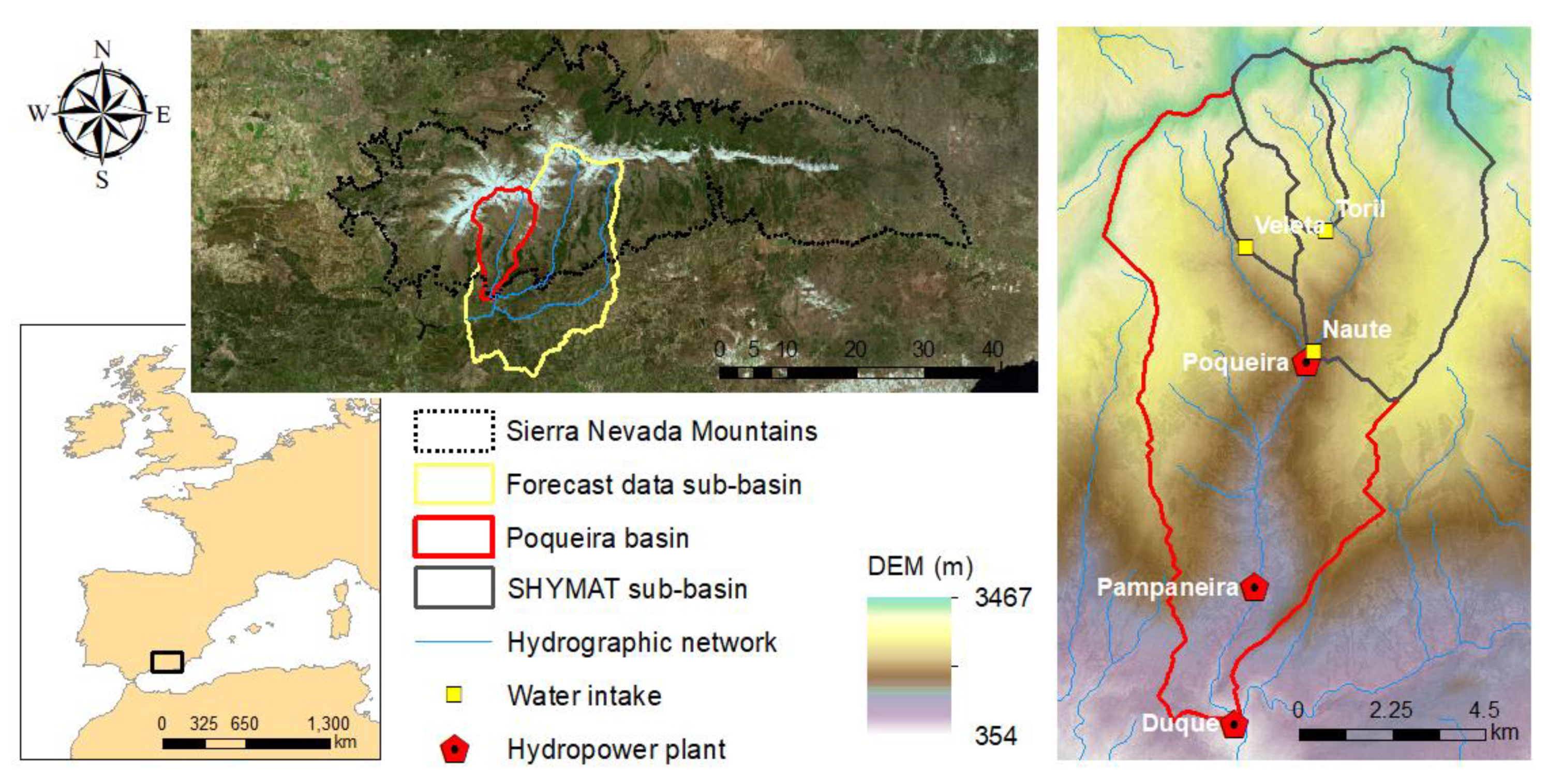
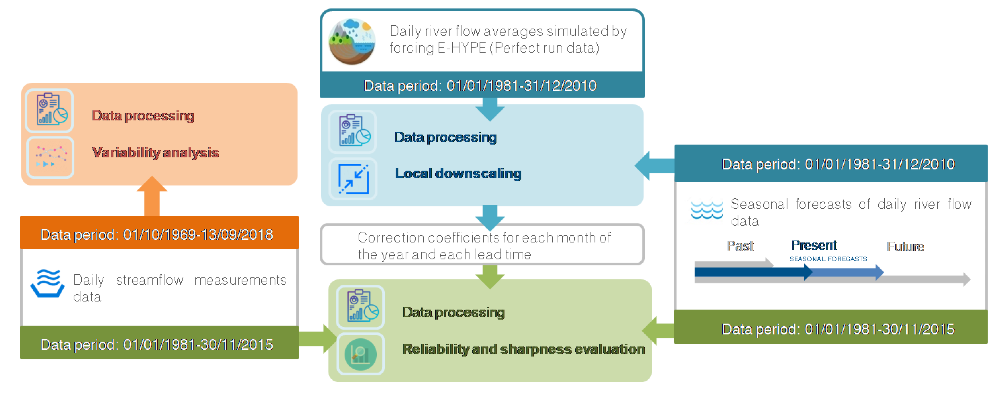
• On one side, seasonal forecasts of daily river flow data (which go up to a six-month prediction horizon) are provided by the Swedish Meteorological and Hydrological Institute (SMHI). The hydrological forecast information is produced by forcing the European Hydrological Predictions for the Environment (E-HYPE) model with data from the European Centre for Medium-Range Weather Forecasts (ECMWF) seasonal forecast systems (SEAS5 and its predecessor System 4) [23,24]. ECMWF systems are based on global climate models, which since the oceanic circulation is a major source of predictability in the seasonal scale, are based on coupled ocean–atmosphere integrations [25]. E-HYPE is the European setup of the HYPE model, which estimates hydrological variables on a daily time step at an average sub-basin resolution of 120 km² [25,26]. For our pilot area, the seasonal forecasts of river flow data produced in a sub-basin of 527 km² were used (Figure 1). Probabilistic forecasts are produced as an ensemble of members or scenarios that present the range of future river flow possibilities. Although the CS is currently operative with SEAS5 data which produces an ensemble of 51 members, in the service testing stage presented here, we used a previous ECMWF seasonal forecast, System 4, for which 15-member hindcasts covering the period 1 January 1981–30 November 2015 for each calendar month and up to six months ahead were available. The sub-basin where E-HYPE river flow forecasts are produced does not perfectly match the contributing area to the pilot three RoR system (see SHYMAT sub-basins in Figure 1). In this work, the raw seasonal forecasts were presented at a monthly scale and statistically downscaled at the pilot local scale to match the temporal and spatial scale suitable for this particular application, as detailed in the Section 2.3.
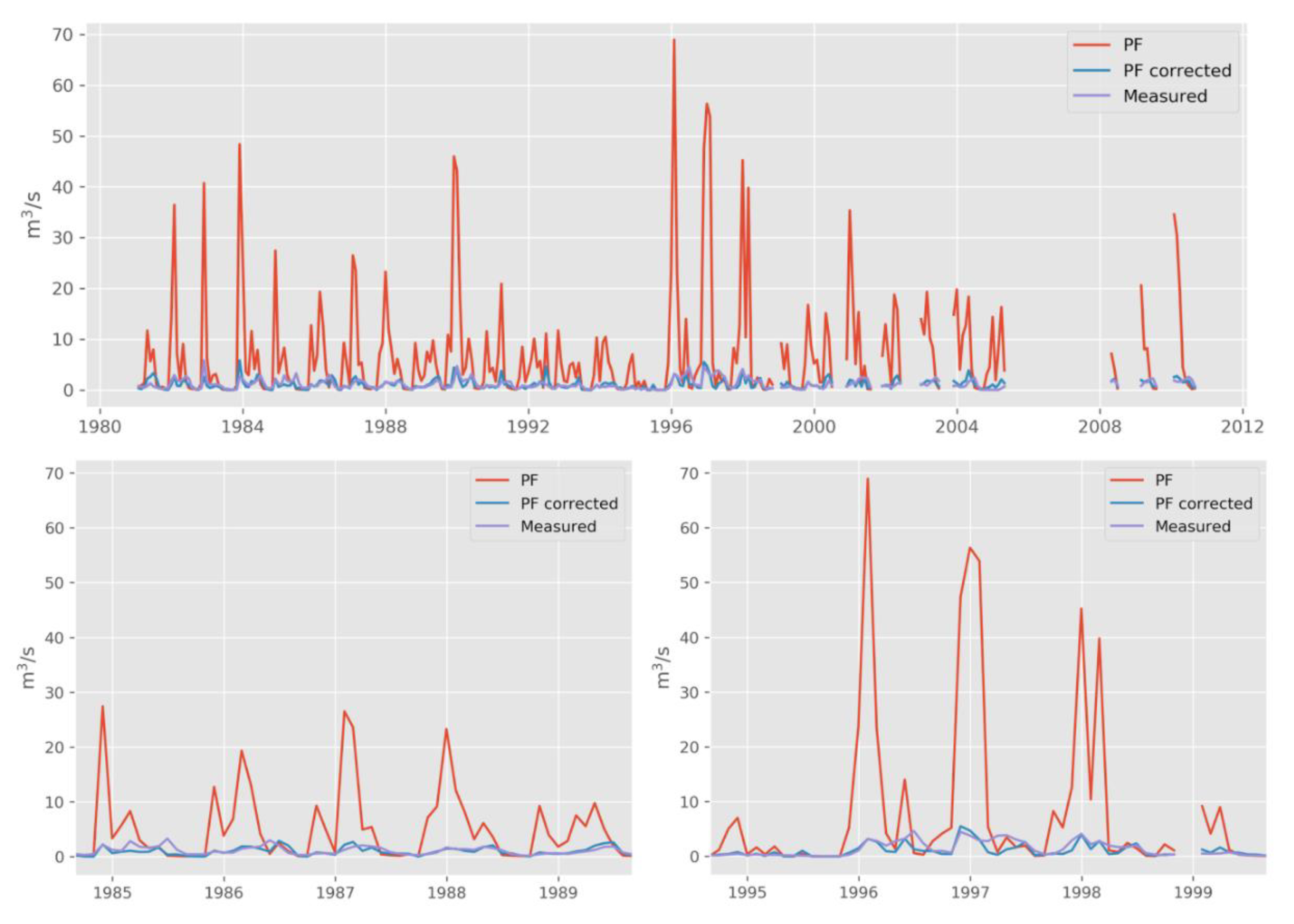
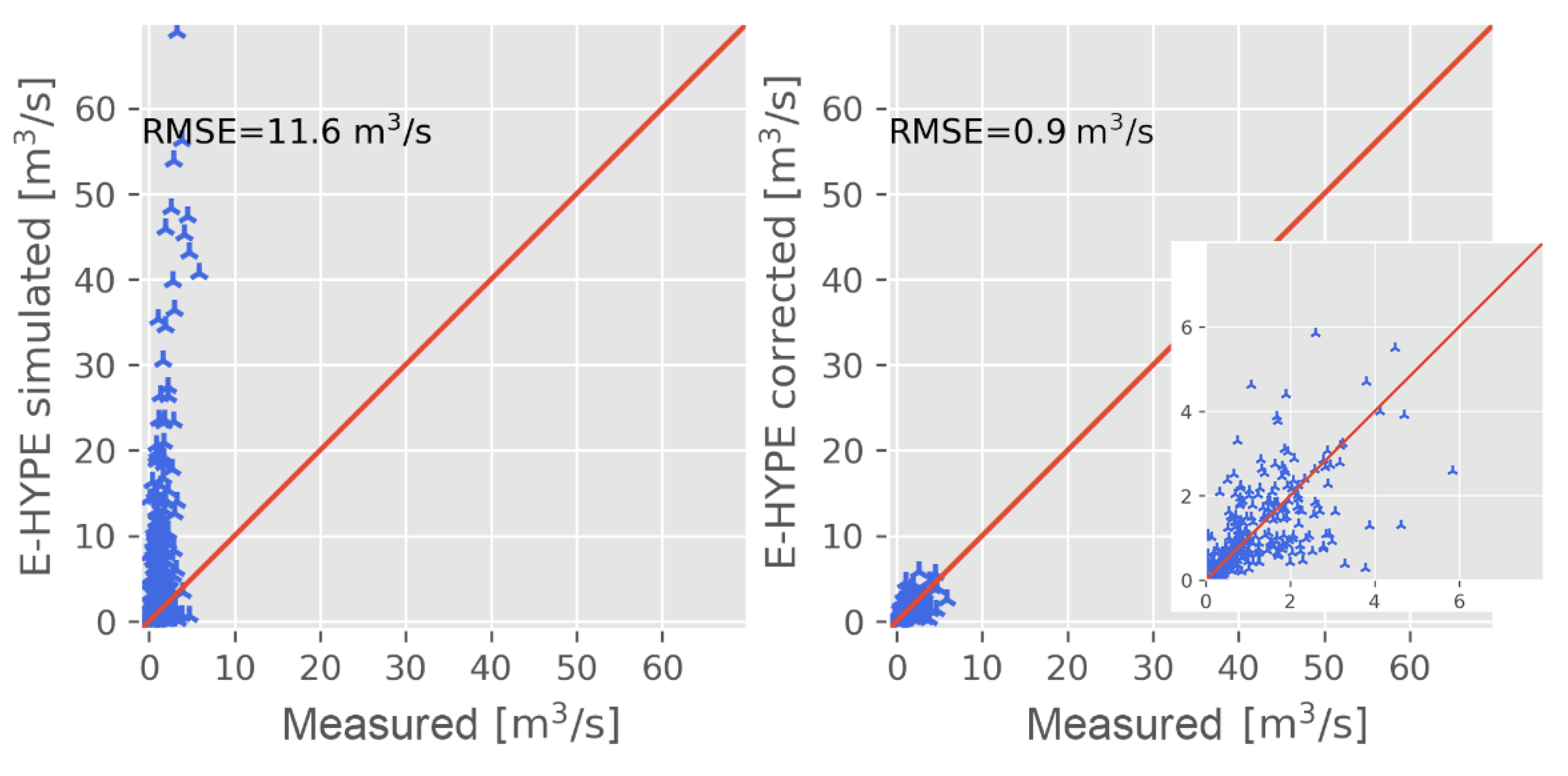
• On the other side, daily river flow averages simulated by forcing E-HYPE with HydroGFD precipitation and temperature coming from reanalyses [27] (perfect run) are available for the period 1 January 1981–31 December 2010.The E-HYPE performance in simulating river flow varies in time and space, with low performance as well as a tendency to overestimate flows in southern Spain [26]. The perfect run data were used in the downscaling step.
• Finally, the daily streamflow measurements for the period 1 October 1969–13 September 2018 in the intake point of the Pampaneira plant (Figure 1), provided by the managers of the hydropower system, give an adequate overview of the historical river inflow to the RoR system and its variability. Data for the Poqueira plant are not available and the data for the Duque plant are normally the same as in the Pampaneira plant, so the results of the analysis can be applied in both plants.

These data series have been used for two different purposes and for each one the longest possible study period according to data availability was considered. The first purpose is to show the high variability of observed inflow data, available for the period 1 October 1969–13 September 2018. For this, daily observed data were processed to compute the monthly inflow data and the results were presented in a color map. The second purpose is the reliability evaluation for each month, for which the three data sources were used. This purpose includes two tasks: (1) downscaling, using perfect run data and streamflow measurements data, both available for the period 1 January 1981–31 December 2010, and (2) the reliability and sharpness evaluation, using seasonal forecast data and streamflow measurements data, both available for the period 1 January 1981–30 November 2015. Figure 2 shows a flowchart of the different methodologies and the data series used.

2.3. Downscaling Approach of Seasonal Forecast Data for Local Application

The spatial and temporal scales of the seasonal data are not suitable to be directly applied in the pilot area. Figure 1 shows on one side the location of the forecast data sub-basin, with an area around 527 km², and on the other side, the contributing area to the pilot three RoR system (SHYMAT sub-basins) estimated around 28.3 km². Thus, the seasonal forecast data need to be statistically downscaled to the intake points of the hydropower plants, adjusting the statistical properties to mimic a higher resolution. For that purpose, we used a quantile mapping method, usually used as a bias-correction method and leading to generally good performance in comparison to other simple bias-correction methods [28,29]. Monthly river flow averages simulated with E-HYPE (perfect run) and river flow measured data for the overlapping period from 1 January 1981 to 31 December 2010 were compared before and after the application of the downscaling methodology. Downscaling parameters based on the quantile mapping method (see Appendix B) were derived by comparing the distributions of E-HYPE-simulated monthly river flows with monthly river flow measurements from 1981 to 2010. These parameters were calculated independently for each month of the year and then used to adjust and downscale the seasonal river flow forecasts month by month from 1981 to 2015.

Figure 3 shows the cumulative distribution function of seasonal forecast data and the measurements for each month of the year, which were used to apply the quantile mapping downscaling and correction methodology. Each peak and spell will receive different corrections, while remaining month dependent. In this way, the melting is still corrected differently than the peak season as they occur in different months.

2.4. Assessment of the Prediction through Seasonal Forecast Data and Historical Data

Seasonal forecasts constitute an added source of information that may help to narrow down the operational options inferred from historical data sources. For these reasons, the assessment exercise enhances the credibility and trust in the information provided by the service. Once seasonal forecast data were downscaled, the evaluation of the prediction of water availability was considered for both (1) the prediction from the CS based on the downscaled seasonal forecast data and (2) the method traditionally used by the water and energy managers in their business as usual, based on an ensemble of historical streamflow measurements [30,31]. In both cases, reliability and sharpness were evaluated.

For the CS prediction, the reliability and sharpness of the seasonal river flow forecasts for all calendar months and the six horizon months were analyzed. Likewise, for traditional prediction, the use of past observations of monthly streamflow measurements from the previous 10 years was assumed. Pilot system managers normally use this historical data period for price market issues, as it includes a sufficiently long period of years to cover at least one complete dry–wet cycle, but does not use too old data that may incorporate long-term trends. For the CS prediction, 15 possible values of monthly river flow are provided for each month, while 10 possible values are considered in the case of traditional prediction.

The methodology followed to assess forecast performance focuses on the sharpness and reliability characteristics. While reliability traditionally characterizes the consistency between the forecast distribution and the observation [11,32], sharpness characterizes forecast spread and is an attribute of forecasts alone, with no regard to corresponding observations [33]. Forecast reliability and sharpness are assessed simultaneously to follow the paradigm introduced by [32], which consists in maximizing sharpness while guaranteeing reliability. Tailored versions of these metrics designed to allow cross-service evaluation, and ease performance communication within services, were applied in this paper [34]. In the case of simplified reliability (S), forecasts are compared with the river inflow measurements by checking whether the observed data fall within the forecast range (defined by the minimum and maximum forecast) estimated for each issue month M_i and target month M_t. If the observation is between the minimum and maximum forecast value, S = 1, otherwise if the observation is outside the forecast range, S = 0.

The reliability thus defined was presented as the percentage of times in which a posteriori observations fell within the prediction range (Equation (1)):

Reliability[M_i, M_t] = mean (S[M_i, M_t])·100,

(1)

where M_i is the issue month, M_t the target month and S the simplified reliability. When this metric is close to 0, the forecast always misses the a posteriori observation, while values close to 100 indicate that the forecast range always covers a posteriori observation.

For sharpness, the spread of the prediction is assessed as the ratio between the average forecast range (s_f) (i.e., the difference between the maximum and minimum forecast values averaged over all forecasts of a given time period) and the average historical range for the same time period (s_h) (i.e., the difference between the maximum and minimum from all available years of the study period). Forecast sharpness is then normalized by the historical sharpness, following Equations (2) and (3)., so that values close to 0 indicate that the forecast is uncertain as the ensemble of historical values and is therefore not considered confident, while the values close to 100 indicate a high confidence of the forecast:

If s_f[M_i, M_t] > s_h[M_i, M_t]; Sharpness[M_i, M_t] = 0,

(2)

Else; Sharpness[M_i, M_t] = 100 − s_f[M_i, M_t] 100/s_h[M_i, M_t].

(3)

Following the aforementioned methodology, the reliability and sharpness for each of the months of the year and for the study period 01/01/1981–30/11/2015 are evaluated.

3. Results

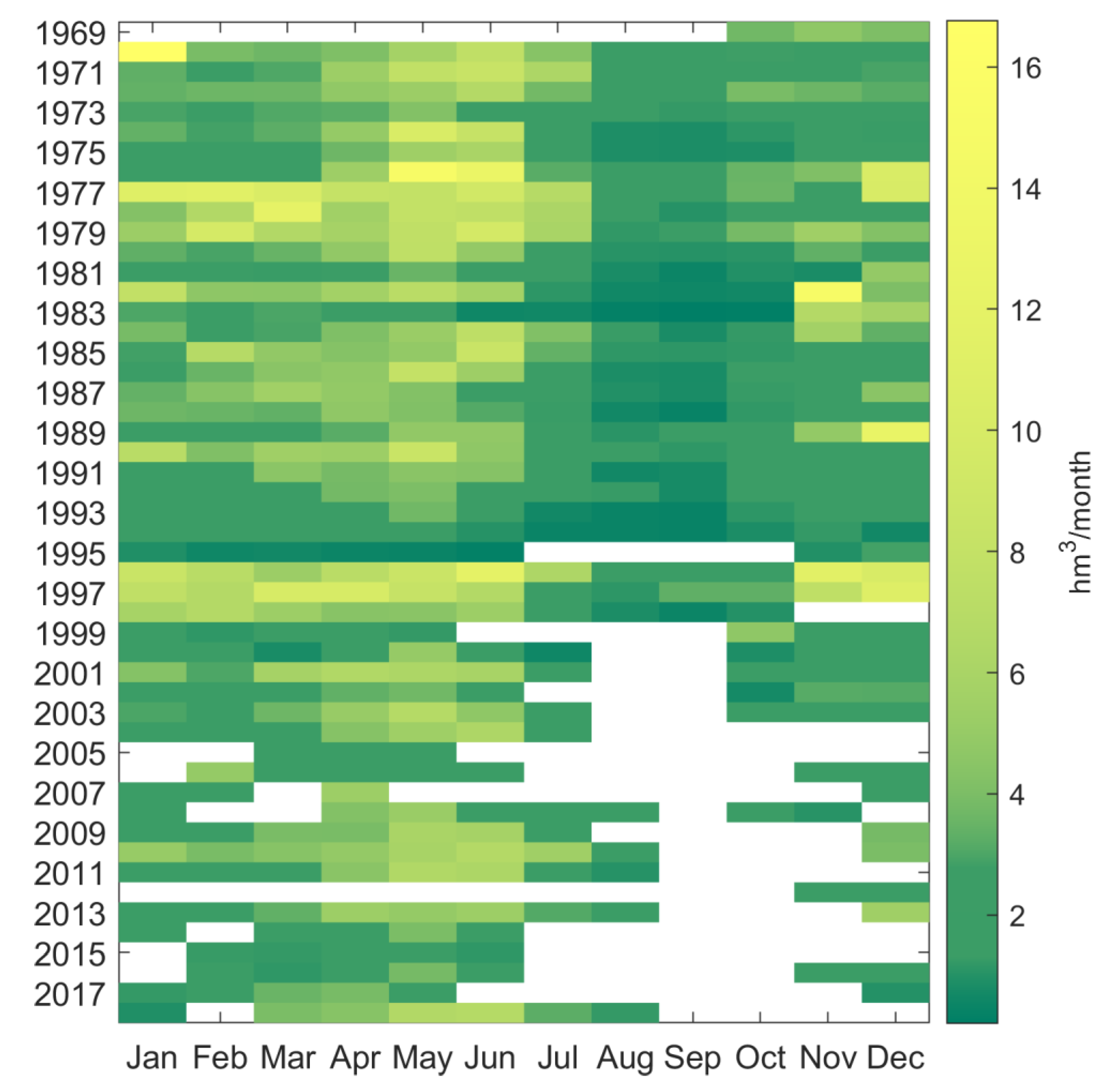
3.1. Variability of Observed Inflow Data

Figure 4 shows a color map displaying the observed monthly inflow data for the study period 1969–2018 in the pilot sub-basin. The map highlights the high variability of river flow through the years, which can vary from 1.1 to 11.6 hm³/month in wet years (1996–1997) and from 0.16 to 1.24 hm³/month in dry years (1994–1995). Moreover, the allocation of high production periods also varies depending on the year. As a clear example, if hydropower managers tried to predict the inflow to the plant for the year 1999 based on historical data, previous years (1996–1998) would induce a high error in the estimation, as these were very wet years. As Figure 4 also shows, the months with high production can vary from year to year: while in 1982, the higher monthly river flow took place around November–January, and in 1986 the higher monthly river flow came about April–June.

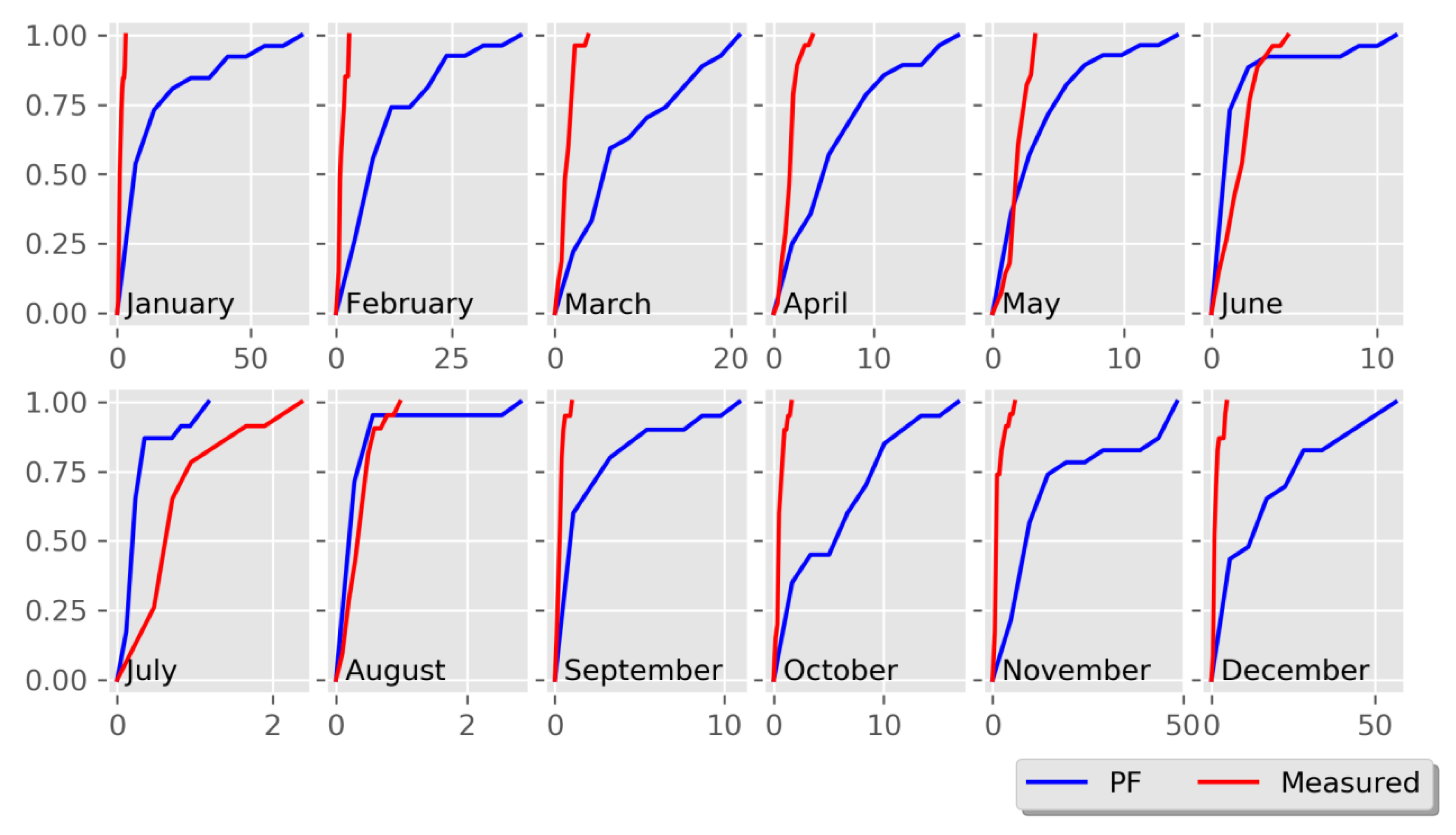
3.2. Downscaling of the Seasonal Forecast Data and Comparison with Measured Data

Before the application of downscaling methodology, the reference simulation of the seasonal forecast and monthly river flow measurements were compared for the period in which both data series overlap, 1 January 1981–31 December 2010. E-HYPE, due to its broad spatial resolution, does not accurately capture the snow processes taking place in this area under the outstanding influence of the high elevation of Sierra Nevada. Thus, snow precipitation is underestimated in favor of rainfall and, consequently, river flow is overestimated in autumn and winter, as shown in Figure 5. Also, spring snowmelt occurs at excessive rates in the model, so the summer river base flow shown by the measurements is not accurately represented.

The quantile mapping method allows to perform the downscaling from the simulated to the real basin, and at the same time to adjust the deviations of the model, mainly linked to the snow simulation. Even though the physical dynamics of the model are not corrected with this method, the resulting series is very close to the actual measurements, as Figure 5 and Figure 6 show. The mean value and the magnitude of the peaks are totally corrected. Moreover, the inconsistencies found in the dynamic operation of the model regarding the snowmelt timing or the performances during the dry years appear to be much improved.

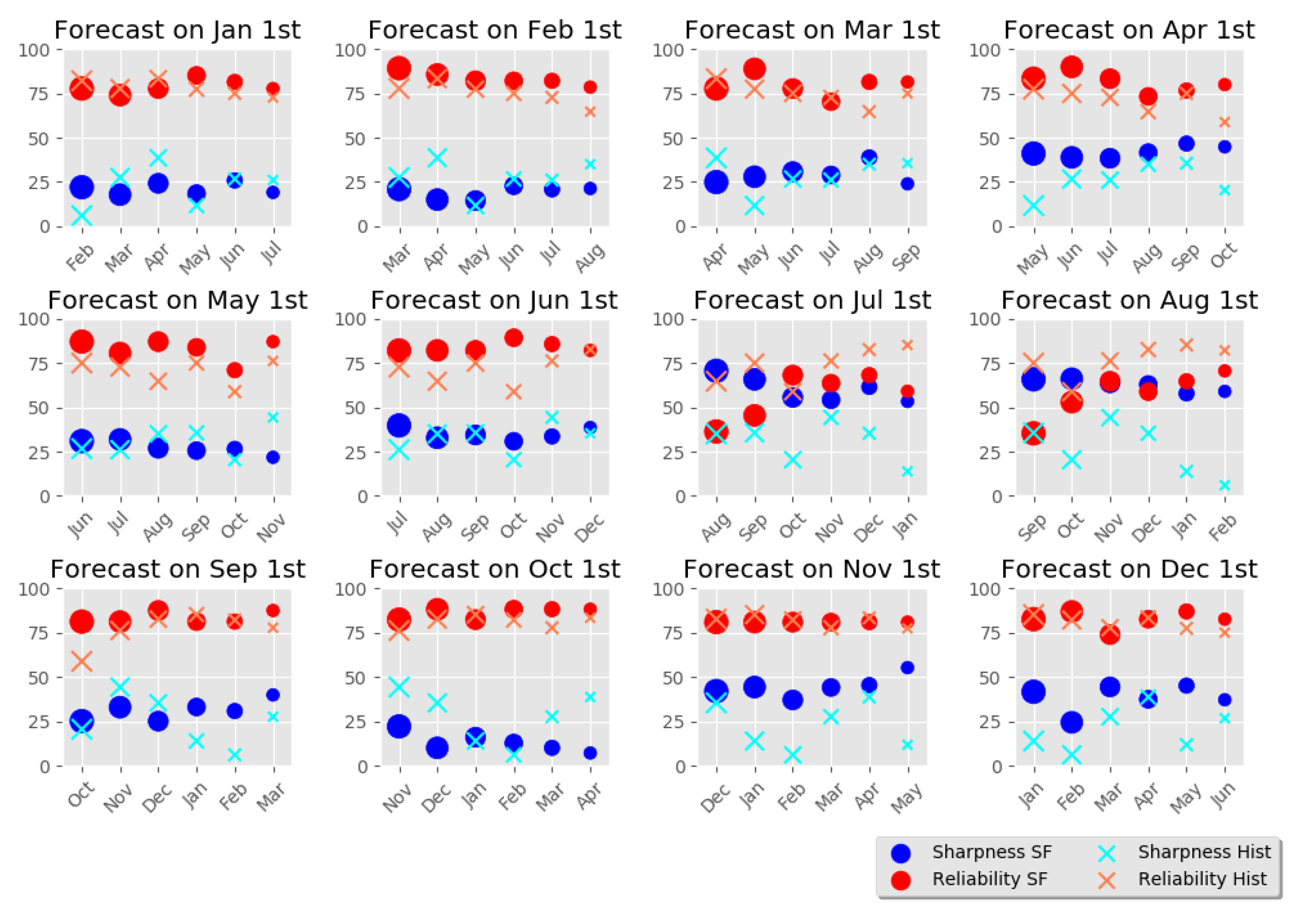
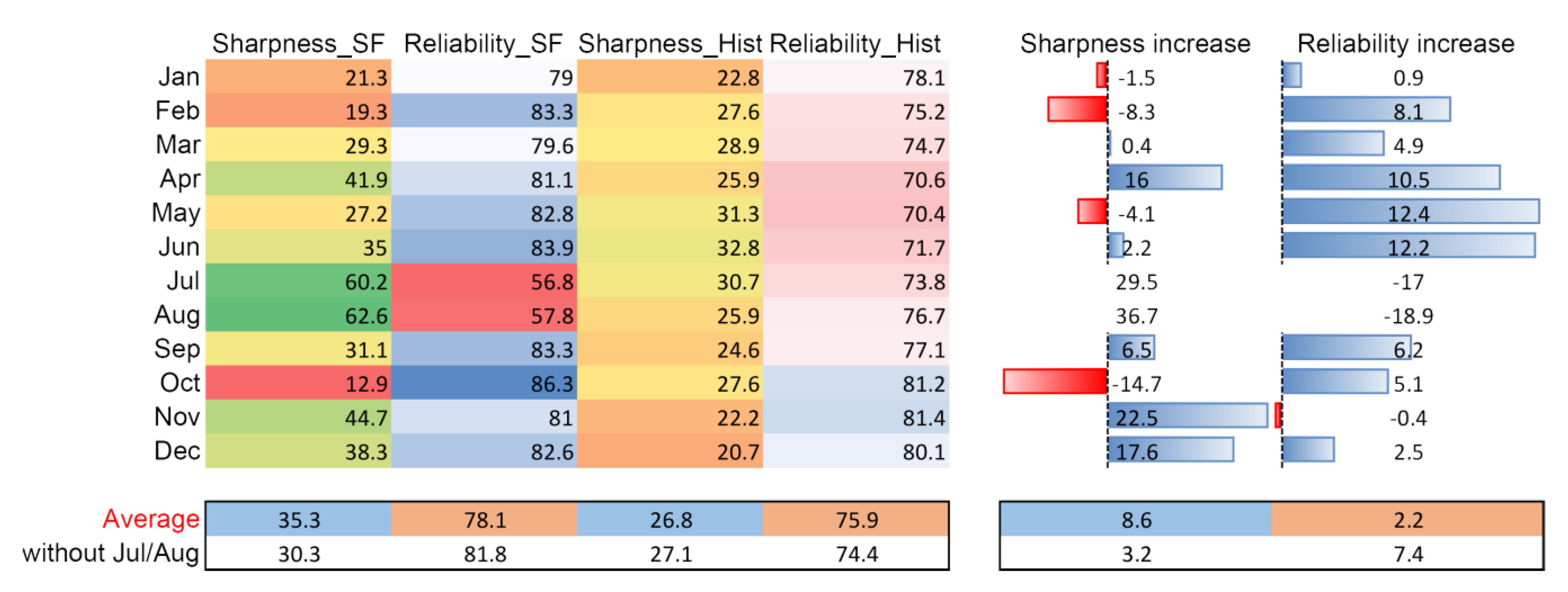
3.3. Evaluation of the Reliability for Each Month

Figure 7 presents, for each month of the year, the reliability and sharpness of the forecasts according to the traditional method and the CS for the six forecast horizons. According to the findings, reliability is higher than sharpness in both prediction methods. The traditional method offers a high reliability along the year. However, the reliability of CS prediction is equal or even higher than the traditional method, even though there are significant differences in the different months and for the different horizons. Particularly, seasonal forecast reliability is consistently higher than that of the traditional method for most of the horizons throughout the year, except for the summer months. This reduction in reliability is closely linked to the exceptionally high values of sharpness obtained in July and August. In these months, the seasonal forecast narrows the range of the predicted values, increasing the sharpness at the expense of reliability. For the rest of the months, the sharpness shows a more erratic distribution over the years, with no clear trend associated with the seasons.

Figure 8 finally shows the numerical values of reliability and sharpness for each month averaged for the six horizons. On one hand, in the case of traditional prediction, average reliability ranges from 70% to 81%, while the CS prediction has an average reliability ranging from 79% to 86% (with the exception of July and August, which show a reliability of 57% and 58%, respectively). These findings mean that seasonal forecast shows an improvement with respect to traditional prediction with an increase in reliability from 5% to 12% in most months, except in the case of the middle of summer, November, January, and to a lesser extent, December. In these summer months, the seasonal forecast reliability clearly decreases by 17%–19%, associated with an increase in sharpness of 30%–37%. These two months show a very particular behavior distinct from the other months, and are thus considered separately in the following analyses. On the other hand, the average sharpness for CS prediction ranges from 15% to 45%, while the traditional prediction average sharpness ranges from 21% to 33%. The total averaged reliability and sharpness show a significant improvement when seasonal forecast is used. If summer months with low reliability are ignored, the averaged reliability and sharpness improve steadily for seasonal forecast (82% and 30%) with respect to historically based prediction (74% and 27%) resulting in sharpness and reliability gains of 3.2% and 7.4%, respectively. It is worth mentioning the case of the spring months, where the sharpness increases by 10%–12% consistently over all the years.

4. Discussion

The operation of the RoR plants should not be only based on historical local data, because of a very high interannual variability of the river streamflow, even more significant in snow areas where the snow cover and processes implied have a large influence on the quantity of water available in the contributing basin. Predictions based on a limited number of previous years cannot predict extreme years (dry or wet) leading to unreliable predictions. This is one of the reasons why energy managers normally tend to consider a historical period of around ten years, which includes wet and dry periods, but even so, it is still an estimation with a high degree of freedom due to the stochasticity of hydrometeorological processes. Thus, seasonal forecast data based on climate model outputs provide a more representative and thus more reliable information while narrowing down the wide window of possibilities that historical data show, verifying the paradigm proposed by Gneiting et al. [32].

The results presented show higher reliability values for the seasonal forecast information than for traditional prediction in most of months, except in the summer months. Thus, the use of seasonal forecast information would improve the prediction of monthly river flow for most of the year, especially in the spring months when seasonal forecast shows both high reliability and sharpness. It should be noted that this differentiated performance for each month’s forecast is generally maintained regardless of the lead time. Spring flows being one of the main resources used in the RoR plants associated with mountain areas, these results show a very high potential benefit for this type of facility.

Predictions showing high sharpness (sharp predictions) imply high confidence, but do not necessarily mean good predictions; as with reliability, sharpness is a necessary and useful but not sufficient condition for high forecast quality [35]. This idea can be applied to the middle of summer, in which a sharp forecast is not reliable. This fact can be due precisely to the higher sharpness shown, because seasonal forecasts try to be excessively sharp, risking for it the reliability of the forecast which implies unrealistic confidence [36]. This is related to the extreme dry summer conditions with almost no precipitation, and hence, no spread in the forecasts of precipitation. As the large-scale hydrological model underestimates the water reserves in the basin in early summer (in the form of soil moisture, groundwater, and to a lesser extent for these dates, snow), low-spread input meteorological forecasts do not manage to perturb the hydrological state either. In this way, the forecasted river flow appears systematically underestimated (as can be seen in the July and August panels in Figure 3) and with very low spread and diminished reliability during the initial lead times of the forecasts made in the summer months (Figure 7).

Although sharpness is not very high, in most cases the seasonal forecast presents a narrower range of possible values than the traditional method and indeed, the total average sharpness found for CS prediction is higher than that found for traditional prediction. In general, it could be said that for equal or less reliability, the use of seasonal forecast information would be an advantage for managers.

To overcome reluctance in the renewable energy sector to apply innovative forecasting CS, attention should be paid in creating confidence and showing the accuracy, skills and uncertainties of the provided forecast. The findings of this work show valuable information that can be applied to the implementation of the CS, taking service developers one step further in the future improvement of the service and providing training for staff to cope with the challenging conditions that future climate scenarios provide to the energy and water sectors. A methodology providing the skill of the forecast information according to the reliability and sharpness values assigned to each month of the year can be suggested as a way to give the user intuitive and accurate information. Thus, according to the results, and if middle summer months (with low reliability) are ignored, the monthly seasonal forecast would be associated with an average reliability around 79%–86%, and a sharpness of around 13%–45%, both depending on the particular month. The outstanding improvement in both metrics achieved in specific months like September, December or the spring months, allows us to glimpse a predictive capacity able to suppose a substantial advantage for the planning of tasks related to the hydroelectric development in rivers of mountainous areas.

This work shows the great influence of the quality of the series of measured data on the skill of the results obtained. On one hand, the measurements are the ground truth that serve to evaluate the success or failure of the forecast models. On the other hand, the measures are also fundamental in the process of bias correction and therefore, determine a great part of the success or failure of the evaluation of the results, beyond the skill of the seasonal forecast. In other words, the application of a seasonal forecast with average or even poor skill over a basin can be enhanced if a good series of measured data, of good length and consistent over time, is available.

Although downscaling methodologies improve the adjustment of seasonal forecast data to measurements, a higher sharpness throughout the months is still needed to narrow the probability of underperformance of the seasonal forecasts that feed the service. Future research must be focused on the improvement of forecast information at the local scale by using both local historical data and high-resolution model outputs with better performance when reproducing the local results.

5. Conclusions

The results confirm the high interannual variability of the river streamflow in the pilot area, and therefore the high error that the predictions of inflow based on historical data can induce, also due to the occurrence of extreme years. In this sense, the use of biased adjusted/downscaled seasonal forecast in the pilot area would provide energy and water managers with more reliable prediction, especially in the spring months, when seasonal forecast shows both high reliability and sharpness. However, the seasonal forecast turned out to be unreliable for the summer months. In general, seasonal forecast information would improve the prediction of observed river streamflow by 7.4% in reliability and 3.2% in sharpness compared to the current operational forecast based on historical data. Finally, seasonal forecasts constitute an added source of information that may help to narrow down the operational options inferred from historical data sources.

References

1. EnAppSys. European Electricity Fuel Mix Summary. Quarterly EU Market Summary, January to March. 2020. Available online: https://b74bc22f-390f-4347-ba45-b13ad13072ee.filesusr.com/ugd/9b26cb_80a91d80583e4c0e8c71ba3211517e3c.pdf (accessed on 20 March 2020).
2. An EU Strategy on Adaptation to Climate Change. Available online: https://climate-adapt.eea.europa.eu/knowledge/tools/adaptation-support-tool/step-1/ressources/cohesion-policy (accessed on 18 March 2020).
3. Adaptation Challenges and Opportunities for the European Energy System. Building a Climate-Resilient Low-Carbon Energy System. Available online: https://www.eea.europa.eu/publications/adaptation-in-energy-system (accessed on 6 April 2020).
4. Dutton, J.A.; James, R.P.; Ross, J.D. Probabilistic Forecasts for Energy: Weeks to a Century or More. In Weather & Climate Services for the Energy Industry; Troccoli, A., Ed.; Springer: Cham, Switzerland, 2018; pp. 161–177. ISBN 978-3-319-68418-5. [Google Scholar]
5. Contreras, E.; Herrero, J.; Crochemore, L.; Pechlivanidis, I.; Photiadou, C.; Aguilar, C.; Polo, M.J. Advances in the Definition of Needs and Specifications for a Climate Service Tool Aimed at Small Hydropower Plants’ Operation and Management. Energies 2020, 13, 1827. [Google Scholar] [CrossRef] [Green Version]
6. Climate Change |Copernicus. Available online: https://www.copernicus.eu/en/services/climate-change (accessed on 1 April 2019).
7. Buizer, J.; Jacobs, K.; Cash, D. Making short-term climate forecasts useful: Linking science and action. Proc. Natl. Acad. Sci. USA 2016, 113, 4597–4602. [Google Scholar] [CrossRef] [PubMed] [Green Version]
8. Polo, M.J.; Contreras, E.; Herrero, J.; Herrera, E.; Mysiak, J.; Larosa, F.; Essenfelder, A.; Santato, S.; Tornato, A. Forum Activity Report III; Climate Forecast Enabled Knowledge Services, 2020; p. 90. Available online: https://drive.google.com/file/d/1EOqm2GTotSLwAHnK5nLpSENGtPyG9UYM/view (accessed on 18 May 2020).
9. Bruno Soares, M.; Dessai, S. Barriers and enablers to the use of seasonal climate forecasts amongst organisations in Europe. Clim. Chang. 2016, 137, 89–103. [Google Scholar] [CrossRef] [PubMed] [Green Version]
10. Palmer, T.N.; Weisheimer, A. On the Reliability of Seasonal Forecasts. In Proceedings of the ECMWF Seminar on Seasonal Prediction, Reading, Berkshire, UK, 3–7 September 2012; pp. 185–194. [Google Scholar]
11. Alessandri, A.; Borrelli, A.; Navarra, A. Evaluation of Probabilistic Quality and Value of the ENSEMBLES Multimodel Seasonal Forecasts: Comparison with DEMETER. Mon. Weather Rev. 2011, 139, 581–607. [Google Scholar] [CrossRef]
12. Kim, H.-M.; Webster, P.J.; Curry, J.A. Seasonal prediction skill of ECMWF system 4 and NCEP CFSv2 retrospective forecast for the Northern Hemisphere winter. Clim.Dyn. 2012, 39, 2957–2973. [Google Scholar] [CrossRef] [Green Version]
13. Weisheimer, A.; Palmer, T.N. On the reliability of seasonal climate forecasts. J. R. Soc. Interface 2014, 11, 20131162. [Google Scholar] [CrossRef]
14. Mishra, N.; Prodhomme, C.; Guemas, V. Multi-model skill assessment of seasonal temperature and precipitation forecasts over Europe. Clim.Dyn. 2019, 52, 4207–4225. [Google Scholar] [CrossRef]
15. Gubler, S.; Sedlmeier, K.; Bhend, J.; Avalos, G.; Coelho, C.A.S.; Escajadillo, Y.; Jacques-Coper, M.; Martinez, R.; Schwierz, C.; de Skansi, M.; et al. Assessment of ECMWF SEAS5 seasonal forecast performance over South America. Weather Forecast 2020, 35, 561–584. [Google Scholar] [CrossRef]
16. Easey, J.; Prudhomme, C.; Hannah, D.M. Seasonal forecasting of river flows: A review of the state-of-the-art. In Climate Variability and Change: Hydrological Impacts, Proceedings of the Fifth FRIEND World Conference, Havana, Cuba, 27 November—1 December 2006; IAHS, Publ.; 308, 158—162; Demuth, S., Gustard, A., Planos, E., Scatena, F., Servat, E., Eds.; IAHS Press: Wallingford, UK, 2006; Available online: http://iahs.info/redbooks/a308/308068.htm (accessed on 29 April 2020).
17. Yuan, X.; Wood, E.F.; Ma, Z. A review on climate-model-based seasonal hydrologic forecasting: Physical understanding and system development. Wiley Interdiscip. Rev. Water 2015, 523–536. [Google Scholar] [CrossRef]
18. Arnal, L.; Cloke, H.L.; Stephens, E.; Wetterhall, F.; Prudhomme, C.; Neumann, J.; Krzeminski, B.; Pappenberger, F. Skilful seasonal forecasts of streamflow over Europe? Hydrol. Earth Syst. Sci. 2018, 22, 2057–2072. [Google Scholar] [CrossRef] [Green Version]
19. Greuell, W.; Franssen, W.H.P.; Biemans, H.; Hutjes, R.W.A. Seasonal streamflow forecasts for Europe—Part I: Hindcast verification with pseudo- and real observations. Hydrol. Earth Syst. Sci. 2018, 22, 3453–3472. [Google Scholar] [CrossRef] [Green Version]
20. Pérez-Palazón, M.J.; Pimentel, R.; Herrero, J.; Aguilar, C.; Perales, J.M.; Polo, M.J. Extreme values of snow-related variables in Mediterranean regions: Trends and long-term forecasting in Sierra Nevada (Spain). Proc. Int. Assoc. Hydrol. Sci. 2015, 369, 157–162. [Google Scholar] [CrossRef] [Green Version]
21. Herrero, J.; Polo, M.J.; Moñino, A.; Losada, M.A. Anenergy balance snowmeltmodel in a Mediterraneansite. J. Hydrol. 2009, 371, 98–107. [Google Scholar] [CrossRef]
22. Pimentel, R.; Herrero, J.; Polo, M.J. Subgrid parameterization of snow distribution at a Mediterranean site using terrestrial photography. Hydrol. Earth Syst. Sci. 2017, 21, 805–820. [Google Scholar] [CrossRef] [Green Version]
23. Crochemore, L.; Ramos, M.-H.; Pechlivanidis, I.G. Can Continental Models Convey Useful Seasonal Hydrologic Information at the Catchment Scale? Water Resour.Res. 2020, 56, e2019WR025700. [Google Scholar] [CrossRef] [Green Version]
24. Pechlivanidis, I.; Crochemore, L.; Bosshard, T. Seasonal streamflow forecasting—Which are the drivers controlling the forecast quality? In Proceedings of the EGU General Assembly 2020, Vienna, Austria, 4–8 May 2020. [Google Scholar] [CrossRef]
25. Molteni, F.; Stockdale, T.; Balmaseda, M.; Balsamo, G.; Buizza, R.; Ferranti, L.; Magnusson, L.; Mogensen, K.; Palmer, T.; Vitart, F. The New ECMWF Seasonal Forecast System (System 4); European Centre for Medium Range Weather Forecasts Shinfield Park: Reading, Berkshire, UK, 2011; Volume 49, Available online: https://www.ecmwf.int/en/elibrary/11209-new-ecmwf-seasonal-forecast-system-system-4 (accessed on 4 March 2020).
26. Hundecha, Y.; Arheimer, B.; Donnelly, C.; Pechlivanidis, I. A regional parameter estimation scheme for a pan-European multi-basin model. J. Hydrol. Reg. Stud. 2016, 6, 90–111. [Google Scholar] [CrossRef] [Green Version]
27. Berg, P.; Donnelly, C.; Gustafsson, D. Near-real-time adjusted reanalysis forcing data for hydrology. Hydrol. Earth Syst. Sci. 2018, 22, 989–1000. [Google Scholar] [CrossRef] [Green Version]
28. Heo, J.-H.; Ahn, H.; Shin, J.-Y.; Rodding Kjeldsen, T.; Jeong, C. Probability Distributions for a Quantile Mapping Technique for a Bias Correction of Precipitation Data: A Case Study to Precipitation Data Under Climate Change. Water 2019, 11, 1475. [Google Scholar] [CrossRef] [Green Version]
29. Crochemore, L.; Ramos, M.-H.; Pappenberger, F. Bias correcting precipitation forecasts to improve the skill of seasonal streamflow forecasts. Hydrol. Earth Syst. Sci. 2016, 20, 3601–3618. [Google Scholar] [CrossRef] [Green Version]
30. Tucci, C.E.M.; Clarke, R.T.; Collischonn, W.; da Silva Dias, P.L.; de Oliveira, G.S. Long-term flow forecasts based on climate and hydrologic modeling: Uruguay River basin. Water Resour. Res. 2003, 39, 1181–1191. [Google Scholar] [CrossRef] [Green Version]
31. Mite-Leon, M.; Barzola-Monteses, J. Statistical Model for the Forecast of Hydropower Production in Ecuador. Int. J. Renew. Energy Res. 2018, 8, 1130–1137. [Google Scholar]
32. Gneiting, T.; Balabdaoui, F.; Raftery, A.E. Probabilistic forecasts, calibration and sharpness. J. R. Stat. Soc. Ser. B 2007, 69, 243–268. [Google Scholar] [CrossRef] [Green Version]
33. Torralba, V.; Doblas-Reyes, F.J.; MacLeod, D.; Christel, I.; Davis, M. Seasonal climate prediction: A new source of information for the management of wind energy resources. J. Appl. Meteorol. Clim. 2016, 56, 1231–1247. [Google Scholar] [CrossRef]
34. Crochemore, L.; Photiadou, C.; Materia, S.; Amadio, M.; Essenfelder, A.H.; Mysiak, J.; Mercogliano, P.; Barbato, G.; Ivars Grape, H.; Cantone, C.; et al. Final Service Development Report and Working Report; Climate Forecast Enabled Knowledge Services, 2020; p. 187. Available online: https://drive.google.com/file/d/1qQO7qdAy7P8LZYt4fH_vHIqNcrUpV9MD/view (accessed on 6 May 2020).
35. Troccoli, A.; Harrison, M.; Anderson, D.L.T.; Mason, S.J. Seasonal Climate: Forecasting and Managing Risk, 1st ed.; Springer: Dordrecht, The Netherlands, 2008; p. 467. Available online: https://books.google.es/books?id=Ga9CAAAAQBAJ&printsec=frontcover&hl=es#v=onepage&q&f=false (accessed on 5 May 2020).
36. Hudson, D. Ensemble Verification Metrics. In Proceedings of the ECMWF Annual Seminar, Reading, UK, 11–14 September 2017. [Google Scholar]
37. Teutschbein, C.; Seibert, J. Bias correction of regional climate model simulations for hydrological climate-change impact studies: Review and evaluation of different methods. J. Hydrol. Reg. Stud. 2012, 456, 12–29. [Google Scholar] [CrossRef]
38. Lucatero, D.; Madsen, H.; Refsgaard, J.C.; Kidmose, J.; Jensen, K.H. On the skill of raw and post-processed ensemble seasonal meteorological forecasts in Denmark. Hydrol. Earth Syst. Sci. 2018, 22, 6591–6609. [Google Scholar] [CrossRef] [Green Version]
Figure 1. Location of the Poqueira River basin in southern Spain and the three run of river (RoR) plants system in the pilot area. The sub-basin where seasonal forecast data are produced and the sub-basins defining the three different points of water uptake for the hydropower production (SHYMAT (small hydropower management and assessment tool) sub-basins) are also presented (from Contreras et al. [5]).
Water 12 02119 g001
Figure 2. Flowchart of the different methodologies applied in this work (variability analysis, local downscaling, reliability and sharpness evaluation) and the data sources used, showing the study periods available for each method.
Water 12 02119 g002
Figure 3. Cumulative distribution functions of the reference simulation (perfect run PF) data and measurements for each month of the year, for the correction period 1981–2010. The x axis represents the average monthly river flow in m3/s.
Water 12 02119 g003
Figure 4. Observed monthly inflow data (hm3/month) for the hydrological period 1969–2018. White spaces represent no-data due to sensor failure.
Water 12 02119 g004
Figure 5. Comparison between monthly average river flow of the reference simulation of European Hydrological Predictions for the Environment (E-HYPE) (perfect run PR) and the measured data for the overlapping period of 1981–2010, before and after the application of downscaling and correction methodology to seasonal forecast data. In the lower plots, the details for a series of dry years (left) and wet years (right).
Water 12 02119 g005
Figure 6. Scatter plot of the monthly mean flow simulated (E-HYPE) versus the measured (provided by the managers of the pilot hydropower system) inflows before and after the quantile mapping downscaling and correction.
Water 12 02119 g006
Figure 7. Reliability and sharpness of the prediction for each month provided by the traditional method (crosses), and the climate services (CS) (circles) for the six horizons, for the study period 1981–2015.
Water 12 02119 g007
Figure 8. Average values for the reliability and sharpness for each month throughout the different lead times according to the Seasonal Forecast (SF) and the traditional method (Hist) (left), and the change of CS prediction reliability and sharpness with respect to traditional prediction reliability and sharpness (right), for the study period 1981–2015.
Water 12 02119 g008