A Comparison and Validation of Saturated Hydraulic Conductivity Models

Abstract

Saturated hydraulic conductivity (K_sat) is fundamental to shallow groundwater processes. There is an ongoing need for observed and model validated K_sat values. A study was initiated in a representative catchment of the Chesapeake Bay Watershed in the Northeast USA, to collect observed K_sat and validate five K_sat pedotransfer functions. Soil physical characteristics were quantified for dry bulk density (bdry), porosity, and soil texture, while K_sat was quantified using piezometric slug tests. Average bdry and porosity ranged from 1.03 to 1.30 g/cm³ and 0.51 to 0.61, respectively. Surface soil (0–5 cm) bdry and porosity were significantly (p < 0.05) lower and higher, respectively, than deeper soils (i.e., 25–30 cm; 45–50 cm). bdry and porosity were significantly different with location (p < 0.05). Average soil composition was 92% sand. Average K_sat ranged from 0.29 to 4.76 m/day and significantly differed (p < 0.05) by location. Four models showed that spatial variability in farm-scale K_sat estimates was small (CV < 0.5) and one model performed better when K_sat was 1.5 to 2.5 m/day. The two-parameter model that relied on silt/clay fractions performed best (ME = 0.78 m/day; SSE = 20.68 m²/day²; RMSE = 1.36 m/day). Results validate the use of simple, soil-property-based models to predict K_sat, thereby increasing model applicability and transferability.

1. Introduction

Saturated hydraulic conductivity (K_sat) is an important hydraulic parameter [1,2,3,4], as K_sat represents the ability of soils to transmit water throughout the saturated zone, which is essential for relating water transport rates to hydraulic gradients [5,6,7]. Accurate K_sat estimates are needed to characterize and predict how soil–water dynamics influence local water balances [8,9,10]. Thus, K_sat estimates can inform resource management decisions related to water conservation, irrigation systems, fertilizer application, drainage, solute mitigation, and plant growth [11,12,13]. Generally, K_sat is measured through field and laboratory techniques (e.g., pumping, permeameter, and slug tests) [14,15,16,17] that are relatively simple to complete [18,19,20]. However, performing a sufficient number of field-based tests may be too expensive, in terms of duration and cost [21,22]. Additionally, field-based K_sat estimates can be limited by incomplete aquifer geometry information, while laboratory methods can present problems with obtaining representative sample numbers. These challenges suggest the need for methods to estimate K_sat that are accurate and efficient [23,24,25].

An alternative to direct K_sat measurements is to predict K_sat with pedotransfer functions [26] that utilize soil physical characteristics such as bulk density [27], porosity [28], particle size fractions [11,29], along with empirical methods that utilize multiple physical properties [30,31,32,33,34,35]. Gathering the required data for physical models is simpler and routinely done, as characterizing soil physical properties is generally less complex than pumping or permeameter tests [36,37,38]. Numerous studies have developed pedotransfer functions to estimate K_sat based on soil properties, as physical characteristics are easily measured and not hydraulic-boundary-dependent [13,32,34]. Many of these simple models utilize one or more soil particle size fractions to directly estimate K_sat [39,40,41] or characterize relationships between additional soil properties and K_sat [11,27]. For example, Saxton et al. [11] showed that the relationships between soil water content and textures resulted in K_sat predictions that compared well with independent K_sat measurements. More complex models, such as Jabro [27], rely on a combination of soil characteristics and particle size fractions to estimate K_sat. More recently, Vienken and Dietrich [14] showed that grain-size data could be adequately used to predict K_sat for initial site assessments, further supporting the use of soil-property-based K_sat models.

Although these studies predicted K_sat using different, widely accepted grain-size metrics and soil characteristics, the results show that soil-property-based K_sat models warrant validation to demonstrate their applicability and transferability. Five previously published models [11,27,39,40,41] present an opportunity for a model validation study, as these models predict K_sat from either one or two particle size fractions and bulk density. More complex models, such as those that utilize grain size distributions [14,30], may result in more accurate K_sat predictions but require additional analyses for adequate model parameterization. These additional steps may not be achievable/affordable for practitioners interested in efficient K_sat predictions [8,42]. However, particle size fractions and bulk density are typically included in soil characterizations and are relatively easy to obtain [13,32], thus supporting the evaluation and comparison of soil-property-based K_sat models. An applied model comparison can determine the accuracy and efficiency of K_sat predictions generated from relatively simple pedotransfer functions.

The importance of accurate K_sat predictions extends beyond validating soil property based K_sat models. K_sat is commonly used to parameterize process based hydrologic models since K_sat governs permeability and contributes to shallow groundwater-surface water exchange processes [17,29]. Many near surface process models (e.g., HEC-HMS) use K_sat as a calibration parameter to understand how water flows change within a specific drainage area [43,44,45]. Additionally, groundwater (e.g., MODFLOW) and solute transport (e.g., ReacTran modeling depends on measures of soil K_sat at specific spatial scales of interest [46,47,48,49]. Thus, accurate K_sat measurements are a prerequisite for simulating flow and transport processes at local levels and up-scaling to regional watersheds [14,50,51].

The primary objective of the current work was to collect observed K_sat values from a representative watershed in the northeastern USA. The sub-objectives were to use observed data to validate the predictive accuracy of the Puckett et al. [39], Jabro [27], Campbell [40], Smettem and Bristow [41], and Saxton et al. [11] K_sat models for coarse-grained, alluvial floodplain soils with a history of agricultural production. Validated model accuracy will improve end-user confidence in model estimated K_sat for use in hydrologic and constituent transport predictions, thus expanding characterizations of local soil–water dynamics. Additionally, these results can increase the applicability of K_sat models for practitioners and improve understanding of local soil–water dynamics.

2. Methods

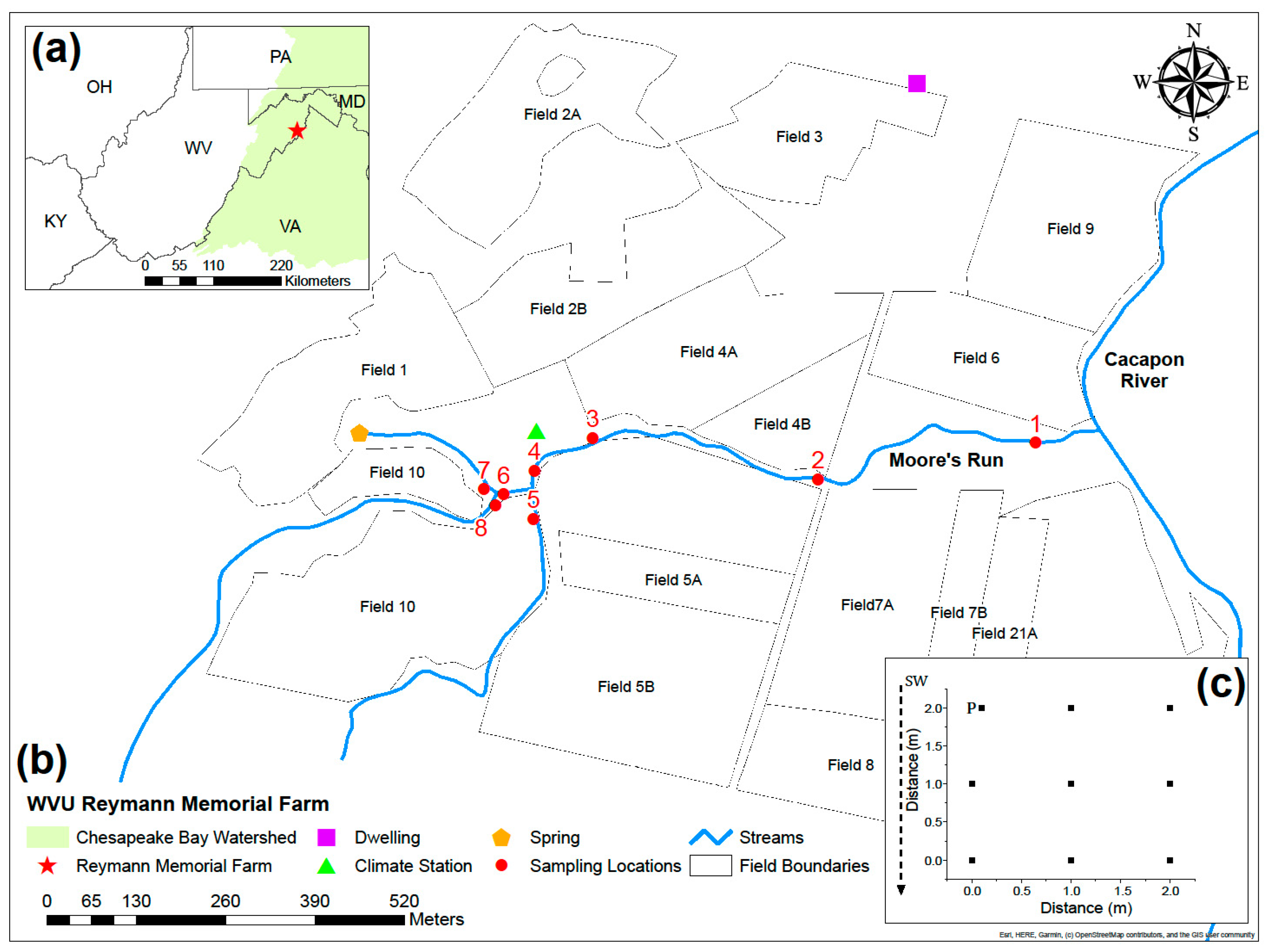
2.1. Site Description

This study was conducted at eight co-located stream stage and piezometer monitoring sites using an experimental watershed study design [52,53,54,55,56,57] along Moore’s Run, located within Reymann Memorial Farm (RMF; 39°6′12.7″ N, 78°35′8.19″ W) near Wardensville, West Virginia, USA (Figure 1). Moore’s Run flows southeast approximately 42 km to the Cacapon River and is in the upper Chesapeake Bay Watershed (CBW) (Figure 1) [58,59,60]. The Cacapon River drainage area is approximately 65.2 km² (

Table 1. Cumulative land use and land cover (LULC) [61] and drainage area (km²) corresponding with each study site (n = 8) sub-basin from the studied portion of Moore’s Run and a sub-watershed of the upper Cacapon River, located near Wardensville, West Virginia, USA ¹. Percent cumulative land use type is displayed parenthetically.

LULC [km2 (%)]	RMF1	RMF2	RMF3	RMF4	RMF5	RMF6	RMF7	RMF8	Cacapon
Agriculture	3.8 (10.5)	3.1 (8.8)	3.1 (8.8)	3.1 (8.8)	2.9 (8.5)	0.2 (20.3)	<0.1 (42.8)	0.1 (16.3)	9.7 (14.9)
Forested	31.1 (86.5)	30.8 (88.3)	30.8 (88.3)	30.8 (88.3)	30.2 (88.5)	0.6 (79.2)	<0.1 (57.2)	0.4 (83.4)	50.8 (77.8)
Mixed Development	0.7 (2.0)	0.7 (1.9)	0.7 (1.9%)	0.7 (1.9)	0.7 (1.9)	<0.1 (0.2)	0 (0)	<0.1 (0.3)	3.1 (4.7)
Open Water	0.4 (1.0)	0.4 (1.1)	0.4 (1.1)	0.4 (1.1)	0.4 (1.1)	<0.1 (0.3)	0 (0)	0 (0)	1.7 (2.5)
Total area	35.9 (100)	34.9 (100)	34.9 (100)	34.9 (100)	34.1 (100)	0.8 (100)	<0.1 (100)	0.5 (100)	65.2 (100)

¹ Site specific drainage areas were delineated using a 1–3 m statewide mosaic for West Virginia [62].

). Land use and land cover (LULC) throughout the upper Cacapon River drainage area is 77.8% forest and 14.9% agriculture (Table 1) [61,62]. Land cover across the contributing drainage area for each study site (n = 8) is similarly dominated by forest and agriculture LULC (Table 1).

The dominant soils in the study area are Basher fine sandy loam in the floodplains and Monongahela silt loam (3–8% slopes) along the stream terraces, with dry bulk density and K_sat ranging from 1.34 to 1.53 (g/cm³) and 0.19–1.99 (m/day), respectively [63,64,65,66]. Natural Resources Conservation Service (NRCS) methods used to derive K_sat typically include double ring infiltrometers, constant head well permeameters, and empirical relationships between dry bulk density and particle size distributions [27,63]. Both soil types are moderately well drained [67]. Particle size fractions for Basher fine sandy loam range from 50 to 90% sand, 6 to 48% silt, and 5 to 12% clay, while average particle size fractions for Monongahela silt loam range from 20 to 27% sand, 51 to 54% silt, and 19 to 26% clay [63]. Regional geology consists of Silurian limestone, Devonian sandstone, Devonian shale, and Quaternary alluvium [68,69]. Soil textures include sand, sandy loam, silty clay loam, silt loam, and loam [63]. A hydroclimate monitoring station was installed at RMF in 2019 as a part of an ongoing nested-scale experimental watershed study (Figure 1) [52,53,54,55,56,70,71,72]. Average daily air temperature (August 2019 to April 2020) was 9.43 °C, while daily precipitation totals ranged from 0 mm to 41.4 mm. Longer term records (1917–2016) show average annual air temperature at the time of observation and average annual precipitation at 8.6 °C was 810.9 mm, respectively [73].

2.2. Soil Strutural Properties

Soil structural properties were determined using the soil core method [37,74]. The soil core method requires the collection of a known soil volume (i.e., core) by driving a cylindrical sampler into the soil to extract relatively undisturbed samples from a series of profile depths. Each core is weighed and then oven-dried at 105 °C for 24 to 48 h, or until the sample mass remains constant with additional drying time [16,75]. The oven-dried sample mass is cooled to room temperature in a desiccator and weighed [37]. At each study site (n = 8), three 98.17 cm³ soil cores (n = 179) were collected from depth intervals of 0–5, 25–30, and 45–50 cm at nine equidistant locations across a 2 m × 2 m grid (Figure 1). The grids were designed to be proximal to the piezometers installed along Moore’s Run [53]. Depth intervals were selected to characterize the soil structural properties of the upper portion of the unsaturated zone. Soil cores could not be collected at every depth/sampling location due to the presence of large rocks.

After sampling, each core was capped at both ends, stored on ice, and transported to the laboratory within 24 h. Each core was processed and analyzed using the following equations from Hillel [37]. Soil dry bulk density, bdry, (g/cm³) was quantified as

$$bdry=\frac{M_s}{V_t},$$

(1)

where M_s (g) is the mass of the soil core solids and V_t (cm³) is the soil core total volume. Porosity (unitless) was estimated as

$$Porosity=\frac{V_f}{V_t},$$

(2)

where V_f (cm³) is the volume of the soil core pore spaces [74,76]. Soil dry bulk density and porosity were quantified because they are structural properties that are known to influence shallow groundwater flow [2,8,38,77] and are easy to measure during routine soil surveys [63]. Two-way analysis of variance (ANOVA) was performed on soil characteristics and tested for significant differences between study site means and independent soil depths [75,78]. After each two-way ANOVA, a Tukey’s post hoc multiple-comparison test compared the nominal and measurement variables in all possible combinations [75,78]. All statistical analyses were performed using Origin Pro 2019 (OriginLab Corporation, Northampton, Massachusetts, MA, USA) software.

2.3. Particle Size Fractions and Soil Texture

After the soil cores were dried and weighed, particle size fraction analysis was performed on the 183 samples using a combination of dry sieving and gravimetric filtration [79,80,81]. Particle size fractions were defined using the NRCS classification system [82]. First, any remaining soil aggregates were carefully broken-up by hand [79,80,81,82,83]. Individual soil core samples were poured into a nest of stacked sieves and separated into three size classes with a mechanical shaker [2,14,81]. The fraction retained on the largest grade sieve (2 mm mesh opening) consisted of coarse gravel, the fraction retained on the fine mesh sieve (53 µm mesh opening) contained sand particles, and the fraction retained in the pan contained fine particles, which consisted of silt and clay [82,84]. After 15 min of sieving, each size fraction was weighed [79,85].

The remaining fine particle fraction was rehydrated with 300 mL of deionized water and vigorously shaken until the particles and the water were well mixed [79,80]. Next, the fine particle mixture was filtered gravimetrically with a vacuum flask [81]. Washed and dried Whatman filter paper (pore size = 2 µm) was used to physically separate the silt and clay size fractions. Filters were oven-dried for one hour at 105 °C, cooled in a desiccator to room temperature, and weighed. The filter drying and weighing process was repeated to confirm that the filtered sample masses agreed within 4% [86]. The mass retained on the filters consisted of the silt fraction [87]. The clay fraction was determined by residual after subtracting the dry-sieved gravel mass, sand mass, and gravimetrically filtered silt mass from the original soil mass [79,81].

The resulting percentages of sand, silt, and clay for each soil core were used to model saturated hydraulic conductivity, as detailed below in Section 2.5. Similar statistical analyses, as detailed in Section 2.2., were conducted on the particle size fraction data. Soil texture was determined for each core using the NRCS Soil Texture Calculator [88].

2.4. Field Saturated Hydraulic Conductivity

A series of falling and rising head slug tests were conducted at the piezometer monitoring locations (n = 8; Figure 1) on 20 September 2019, 20 January 2020, and 6 March 2020, to determine K_sat (m/day). Steel drive point piezometers 0.61–1.52 m long with a 3.18 cm inner diameter and a 0.77 m screened bottom segment (i.e., drive point) were driven into the unconfined alluvial aquifer at RMF. Each piezometer was equipped with a Solinst Levelogger Edge [89] pressure transducer to measure water level (M5: error ± 0.003 m; M10: error ± 0.005 m) either every 0.125 s or 0.5 s for the duration of the slug tests. The difference in sampling interval was due to the length of time required for each test and instrument storage capacity. After enough time (i.e., 5–10 min) passed for the water level to equilibrate with the added sensor, a 0.17 cm³ copper slug was quickly lowered into and removed from each piezometer three times, with time allowed for water levels to equilibrate between each slug insertion and retrieval. Based on earlier field tests, water levels were estimated to equilibrate after a period of at least 5 min. Steady state conditions between replicate slug tests were visually confirmed by identifying asymptotes in the water level data. Average K_sat were calculated from the falling and rising water levels using Hvorslev’s method [15,17]

$$K_{sat}=\frac{r^{2}ln\left(L_e/R\right)}{2L_e{t}_{37}}$$

(3)

where r is the radius of the well casing (cm), R is the radius of the well screen (cm), L_e is the length of the well screen (cm), and t₃₇ (s) is the time it takes for the water level inside the piezometer to rise or fall 37% of the initial change during a slug test. It should be noted that the average K_sat derived from slug tests requires the assumption that the average K_sat is representative of the actual field conditions [23].

Falling and rising head slug tests were conducted to assess whether K_sat varied during the piezometer emptying and filling as water levels returned to static conditions. Thus, a significant difference in falling- and rising-head-derived K_sat demonstrates the presence of a directional dependence on the slug test type that may be attributed to site non-idealities [18]. Slug tests were repeated to increase the statistical power of the results [19]. Differences between the average (n = 3) falling-head-derived K_sat and average rising-head-derived K_sat (n = 3) were tested with a paired sample T-test [78]. Differences in site-average K_sat (n = 6), independent of slug test type, were quantified with a one-way ANOVA and a Tukey’s post hoc multiple-comparison test compared pairs of site-average K_sat in all possible combinations [78].

2.5. Modeling Saturated Hydraulic Conducitivity

Average site-level K_sat was estimated using soil particle size fraction data and five previously published pedotransfer functions [11,27,39,40,41], with the understanding that K_sat predictions reflect neither horizontal nor vertical aquifer properties due to the nature of the soil core sampling procedure [90]. Studies have shown that floodplain soil characteristics converge at depths of approximately 50 cm [75,91], which supports K_sat predictions based on data from shallower (i.e., <50 cm) depths. Model results were compared to average measured K_sat. Rising and falling head slug tests were combined so that each average measured K_sat was based on a larger sample size (n = 6) to increase statistical power and capture unsaturated zone water flow variability. The resulting average K_sat for each study site accounted for soil wetting and drying. Model performance was evaluated by comparing predicted K_sat to measured K_sat at the farm-level.

2.5.1. Puckett et al. Model

Puckett et al. [39] developed a model to predict K_sat based on only clay-sized particles. The authors showed that fine sand, sand, and clay percentages were highly correlated with K_sat, surface area, and volumetric water content at specific pressure heads [39,82]. The model for estimating K_sat based on clay fractions is as follows

$$K_{sat}{\left(p\right)}_i=4.66\ast {10}^{-3}exp\left(-0.1975clay\right)$$

(4)

where K_sat (p)_i is the predicted soil saturated hydraulic conductivity (cm/s) at each study site (i) and clay represents the average dimensionless clay fraction.

2.5.2. Jabro Model

Jabro [27] proposed a model that used bdry and grain size as predictive variables of K_sat

$$log\left[K_{sat}{\left(p\right)}_i\right]=9.59-0.81log\left(silt\right)-1.09log\left(\mathrm{clay}\right)-4.64\left(bdry\right)$$

(5)

where K_sat (p)_i is the predicted soil saturated hydraulic conductivity (cm/h) from each site (i); silt and clay represent site-average dimensionless fractions of silt and clay, respectively; and bdry is the site-average dry bulk density (g/cm³).

2.5.3. Campbell Model

Campbell [40] published a model to predict K_sat from existing soil texture data

$$K_{sat}{\left(p\right)}_i=C\ast exp\left[-0.025-3.63\left(silt\right)-6.9\left(clay\right)\right]$$

(6)

in which K_sat (p)_i is the predicted soil saturated hydraulic conductivity (mm/h) from each site (i). Silt and clay represent site average dimensionless fractions of silt and clay, respectively. The constant C is equal to 144 and was derived from previously published studies by Hall et al. [92] and Smettem and Bristow [41].

2.5.4. Smettem and Bristow Model

Smettem and Bristow [41] developed a model to predict K_sat from soil clay content using a variety of agricultural topsoil samples [13]. The two-equation K_sat model is as follows

$$h_b=43.5/\left[-0.25log\left(clay\right)+0.5\right]$$

(7)

$$K_{sat}{\left(p\right)}_i=2500\ast C\ast h_b{}^{-2}$$

(8)

where h_b is the bubbling pressure (mm), clay represents the average dimensionless fraction of clay, and K_sat (p)_i is the predicted soil saturated hydraulic conductivity (mm/h) at each study site (i). The constant, C, in Equation (8) is the same constant as Equation (6).

2.5.5. Saxton et al. Model

Saxton et al. [11] studied the relationships between soil texture and soil moisture content at saturation (Equation (12)) and soil texture and K_sat (Equation (9)). The relationships between these parameters and K_sat are

$$K_{sat}{\left(p\right)}_i=2.778\ast {10}^{-3}\left\{exp\left[A+\left(B/{\theta }_s\right)\right]\right\}$$

(9)

$$A=12.012-0.0755\left(sand\right)$$

(10)

$$B=-3.8950+0.03671\left(sand\right)-0.1103\left(clay\right)+8.7546\ast {10}^{-4}{\left(clay\right)}^2$$

(11)

$${\theta }_s=0.332-7.251\ast {10}^{-4}\left(sand\right)+0.1276log\left(clay\right)$$

(12)

where K_sat (p)_i is the predicted soil saturated hydraulic conductivity (mm/s) at each study site (i); sand and clay represent the average dimensionless fraction of sand and clay, respectively; and θ_s is the soil moisture content at saturation (m³/m³).

2.5.6. Statistical Analysis

Farm-level predicted and measured K_sat were compared for each K_sat model using a statistical analysis outlined in Duan et al. [13]. The mean error (ME), the sum of squared error (SSE), and the root of the mean-square error (RMSE) were quantified for each model. The mean difference between the average predicted and average measured values was determined for the ME with

$$ME={\displaystyle \sum }_{i=1}^n\frac{K_{sat}{\left(p\right)}_i-K_{sat}{\left(m\right)}_i}{n}$$

(13)

where K_sat (m)_i is the measured soil-saturated hydraulic conductivity (m/day) from each of study site (i); K_sat (p)_i is the predicted soil-saturated hydraulic conductivity (m/day) from each of study site (i); and n is the number of sites included the farm-level metrics (n = 8). The SSE and RMSE were determined using the following equations

$$SSE={\displaystyle \sum }_{i=1}^n{\left[K_{sat}{\left(p\right)}_i-K_{sat}{\left(m\right)}_i\right]}^2$$

(14)

$$RMSE=\sqrt{\frac{{{\displaystyle \sum }}_{i=1}^n{\left[K_{sat}{\left(p\right)}_i-K_{sat}{\left(m\right)}_i\right]}^2}{n}}.$$

(15)

3. Results and Discussion

3.1. Soil Structural Properties

Soils cores were extracted at depths of 0–5, 25–30, and 45–50 cm within the 2 m × 2 m study grid (Figure 1c), for a total sample size ranging from 14 to 27 at each study site (n = 179, total core number). The average soil core results for bdry and porosity over the total depth (50 cm) were 1.11, 1.25, and 1.29 g/cm³ and 0.58, 0.53, and 0.51, respectively (Figure 2). Mean bdry ranged from 1.03 g/cm³ at RMF7 to 1.30 g/cm³ at RMF5 and RMF8, with an eight site mean of 1.21 g/cm³. Mean porosity ranged from 0.51 at RMF4, RMF5, and RMF8 to 0.61 at RMF7, with an eight site mean of 0.54. Average bdry was below the NRCS range for the region (i.e., 1.34–1.54 g/cm³) but within the range expected for sandy soils [63,93]. The average porosity values were within the expected soil range of 0.3–0.7 [94]. The differences in bdry were likely due to differences in sampling locations for the NRCS study.

Based on two-way ANOVA results, sites differed significantly in bdry (n = 179; p < 0.05). A comparison of the sites sampled at all depths, using Tukey’s post hoc multiple comparison, showed that bdry was significantly lower at the 0–5 cm depth (n = 14 to n = 27 each site; p < 0.05) [78]. Porosity was also significantly different among study sites (n = 179; p < 0.05) and was significantly higher (n = 14 to n = 27 each site, p < 0.05) at the 0–5 cm depth. bdry and porosity were statistically similar (p > 0.05) at 25–30 and 45–50 cm, confirming that below the surface (i.e., 0–5 cm), RMF alluvial soils are homogeneous [75,91]. However, significant differences (p < 0.05) in RMF bdry and porosity are evidence of inter-site heterogeneity between RMF study sites.

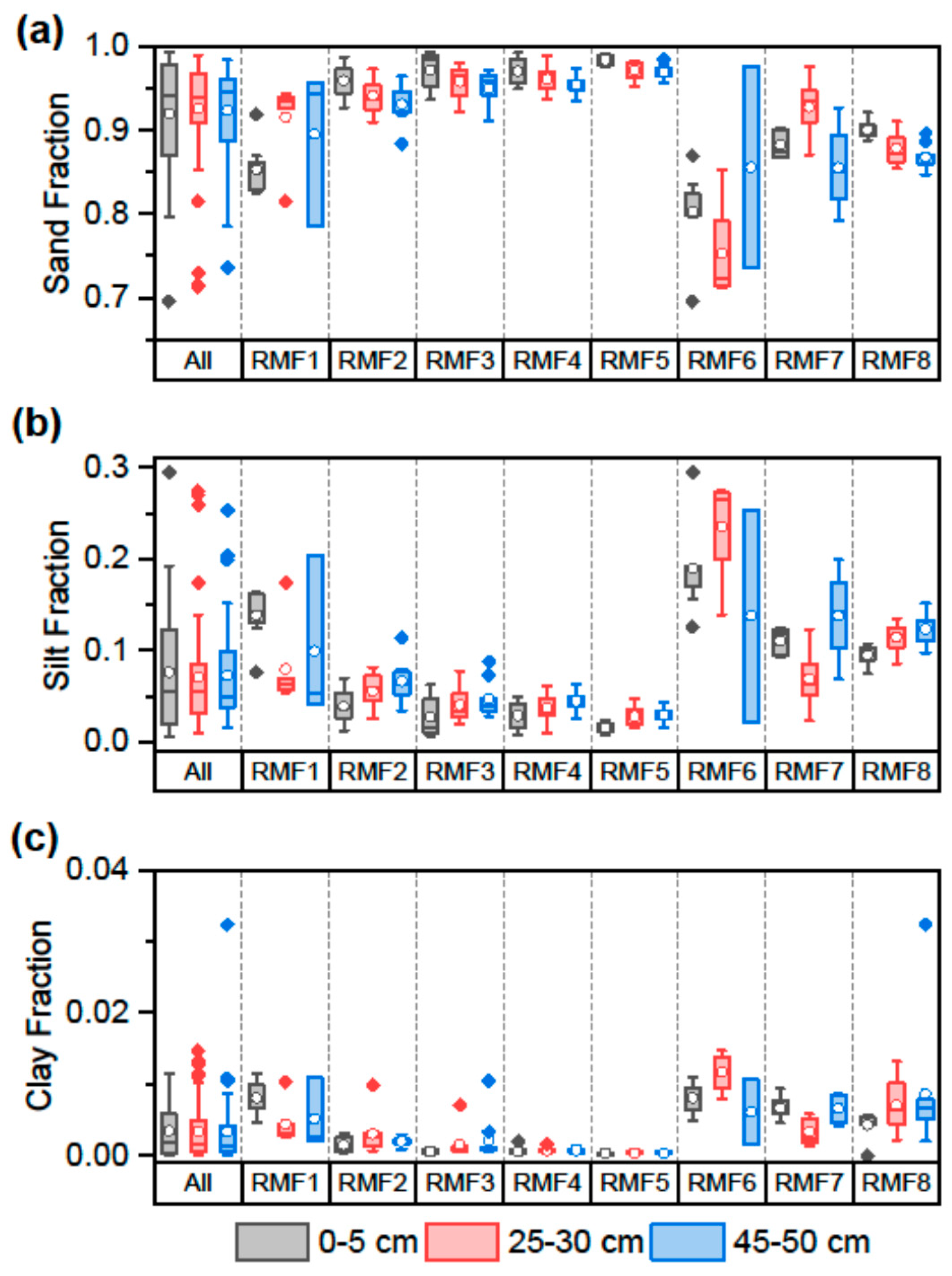
3.2. Particle Size and Soil Texture

When particle size classes (i.e., sand, silt, and clay) were averaged over the total depth (50 cm), sand was consistently the dominant particle size class, followed by silt, and then clay. Average (n = 179) sand, silt, and clay percentages were 92%, 7%, and <1%, respectively (Figure 3). Based on the results of two-way ANOVA tests, the sites differed significantly in all particle size classes (n = 179; p < 0.05) [78]. The soil core textures were sand (n = 155) with a few instances of loamy sand (n = 24) [63]. A comparison of the particle size fractions at all sampled depths with Tukey’s post hoc multiple comparison tests showed that the sites did not differ significantly in average particle size class percentages between soil depths (p > 0.05) [78]. When comparing these results to NRCS-mapped soils from the Web Soil Survey, which included higher percentages of silt and clay fractions, RMF soils had higher sand percentages, and smaller silt and clay percentages [63].

Results confirm that site soil textures were mostly comprised of sand but differed from NRCS findings, which include larger silt and clay fractions (Figure 3) [63,64]. This could be due to the proximity of the sampling grids to Moore’s Run and is evidence of inter-site particle size heterogeneity across RMF study sites and the NRCS sampling locations. Differences in particle size fraction percentages with increasing depth were not significant (p > 0.05), which supports the use of near-surface (i.e., ≤50 cm) particle size fraction data to model K_sat values in the current work.

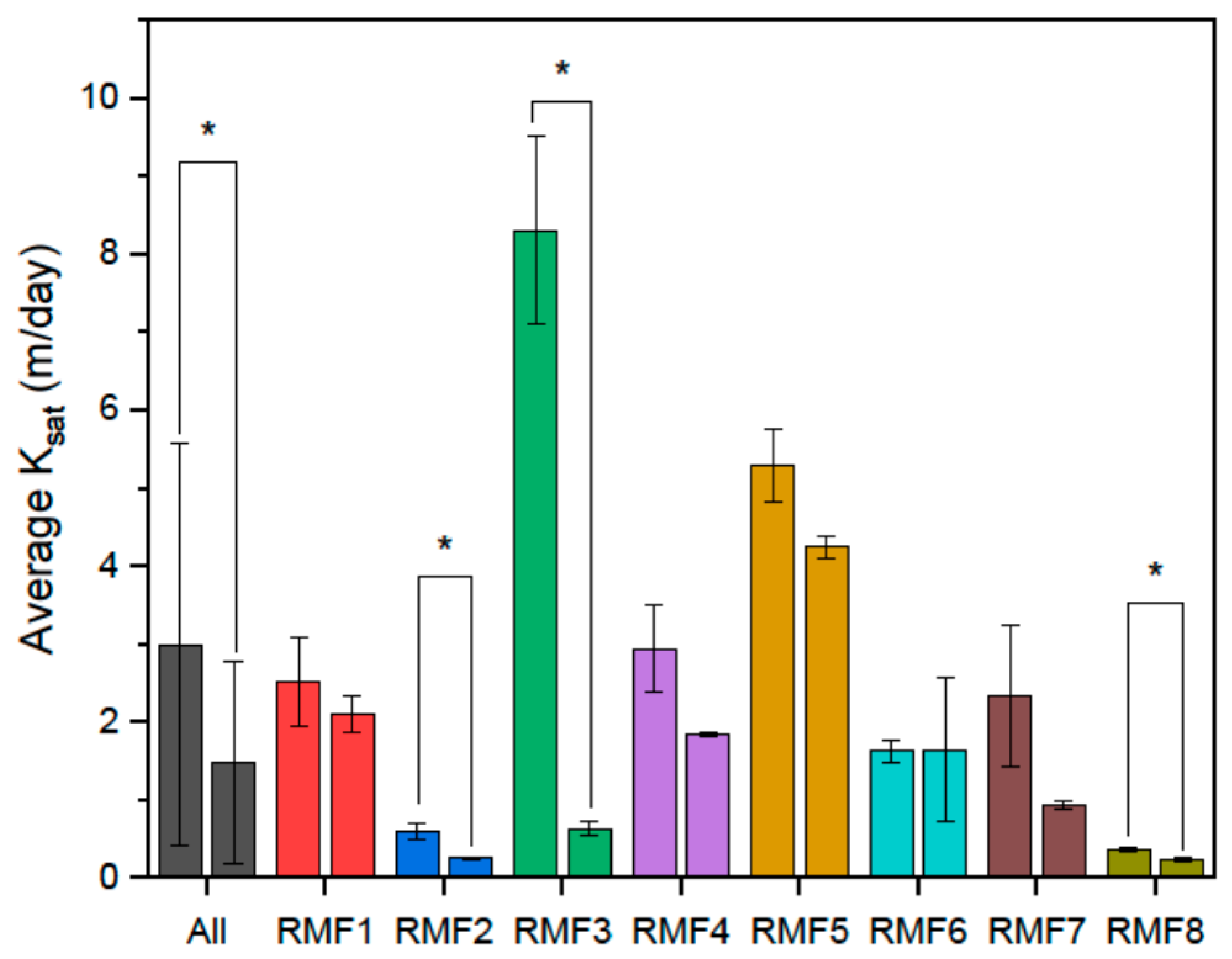
3.3. Field Saturated Hydraulic Conductivity

Site-level comparisons of slug-test-derived K_sat are presented in Figure 4 and separated by slug test type (i.e., FH or RH). FH K_sat were typically higher than RH K_sat, except for RMF6, where FH and RH K_sat were similar. The differences in K_sat between the slug test type can be attributed to non-idealities such as well-skin effects [18,19], while the similar K_sat values at RMF6 may be explained by differing non-idealities at this site. However, these differences may be attributed to the unique soil properties and site features adjacent to the RMF6 piezometer. A Tukey’s post hoc multiple comparison of piezometer adjacent soils revealed that particle size fractions at RMF6 were significantly different (p < 0.05) when compared to RMF4 and RMF5, while the RMF6 clay fraction was significantly different (p < 0.05) from RMF3 [78]. Additionally, the piezometer at RMF6 was proximal to a buried culvert pipe that may have created an artificial hydraulic boundary, resulting in FH and RH K_sat estimates that were different from the other sites.

Observed K_sat values across all study sites ranged from 0.35–9.33 m/day and 0.21–4.37 m/day for FH and RH slug tests, respectively. The larger range in FH K_sat may be attributed to more variable flow resistance during the FH slug tests [18,95]. When compared across all sites (n = 24 per slug test type), FH and RH K_sat values were significantly different (p < 0.05) (Figure 4) [78]. When examined by site (n = 3 per slug test type), RMF2, RMF3 and RMF8 had significantly different FH and RH K_sat (p < 0.05), likely due to differences in flow resistance near the piezometer screened interval [18,19,95,96]. When compared to the expected average K_sat for the region, five average FH K_sat were higher than K_sat range reported by the NRCS of 0.19–1.99 m/day, while only two average RH K_sat were higher than the expected range [63,64]. These differences in K_sat range may be due to methodology, as NRCS uses double ring infiltrometers and constant head well permeameters for field K_sat [97], while soil core bdry and particle size distributions are used for laboratory K_sat estimates [27].

Site-level average K_sat ranged from 0.29 m/day at RMF8 to 4.76 m/day at RMF5, while the average farm-level K_sat was 2.24 m/day (

Table 2. Site-level soil saturated hydraulic conductivity (m/day) comparisons derived from the falling head and rising head slug tests. The coefficient of variation (CV) is presented as a unitless ratio of the standard deviation to the mean.

Site	n	Mean	Med	Std. Dev.	CV
All	48	2.24	1.80	2.15	0.96
RMF1	6	2.31	2.23	0.45	0.19
RMF2	6	0.43	0.39	0.20	0.46
RMF3	6	4.46	3.85	4.27	0.96
RMF4	6	2.39	2.22	0.70	0.29
RMF5	6	4.76	4.56	0.65	0.14
RMF6	6	1.63	1.54	0.58	0.36
RMF7	6	1.63	1.14	0.96	0.59
RMF8	6	0.29	0.30	0.08	0.26

). The results of a one-way ANOVA indicated that the site-level average K_sat were significantly different across all study sites (n = 8; p < 0.05) [78]. Tukey’s post-hoc multiple comparison test showed that average measured K_sat at RMF 3 and RMF5 were significantly higher than RMF2 and average measured K_sat at RMF5 was significantly higher than RMF6, RMF7, and RMF8 (p < 0.05). These significant differences highlight the inter-site heterogeneity between RMF study sites [78]. Since site-level average K_sat include FH and RH slug test variability, and thus better capture heterogeneity, they were used to assess K_sat model performance. Site-level average K_sat coefficient of variation (CV) ranged from 0.19 at RMF1 to 0.96 at RMF3, indicating greater variation between slug tests at RMF3. The greater variability in measured K_sat at RMF3 likely contributed to the high farm-level CV (Table 2) when all measure K_sat were averaged (n = 48).

3.4. Modeled Saturated Hydraulic Conductivity

Predicted site-level K_sat and descriptive statistics for farm-level K_sat are presented in

Table 3. Site-level soil saturated hydraulic conductivity (m/day) comparisons estimated using five K_sat models [11,27,39,40,41], the resulting farm-level descriptive statistics, and additional model information including data source location(s), type of model parameters(s), and the number of estimated model parameters. The coefficient of variation (CV) is presented as a unitless ratio of the standard deviation to the mean.

Site	Puckett et al.	Jabro	Campbell	Smettem and Bristow	Saxton et al.
RMF1	3.55	6.24	2.14	5.03	2.52
RMF2	3.86	20.72	2.74	6.22	2.52
RMF3	3.92	48.68	2.91	6.73	2.27
RMF4	3.97	54.17	2.94	7.61	1.07
RMF5	4.00	168.07	3.08	8.60	0.29
RMF6	3.39	1.04	1.56	4.70	1.77
RMF7	3.58	11.84	2.14	5.09	2.45
RMF8	3.53	1.84	2.15	4.98	2.60
Mean	3.72	39.07	2.46	6.12	1.94
Std. Dev.	0.24	56.00	0.53	1.43	0.84
CV	0.06	1.43	0.22	0.23	0.44
Location(s)	AL, USA	PA, USA	England/Wales	Australia	USA
Parameter(s)	clay	silt, clay, bdry	silt, clay	clay	sand, clay
Parameter #	1	3	2	1	2

for the Puckett et al. [39], Jabro [27], Campbell [40], Smettem and Bristow [41], and Saxton et al. [11] models. Average farm-level K_sat predicted by five tested models ranged from 1.94 m/day with the Saxton et al. [11] model to 39.07 m/day with the Jabro [26] model (Table 3). When compared to the observed farm-level K_sat (Table 2), the Puckett et al. [39], Campbell [40], and Saxton et al. [11] models resulted in estimated K_sat within one standard deviation of the average farm-level K_sat and were similar in magnitude. The Smettem and Bristow [41] model resulted in an estimated K_sat within two standard deviations of the farm-level K_sat. The Jabro [27] model, which was the only model that included bdry as a model parameter, resulted in an unrealistically high K_sat that was 178% higher than the observed result. Differences between model results may be attributable to the soil texture range of samples used in the previous studies or the topographic position of the sampling sites. Additionally, the inclusion of additional model parameters did not always result in a lower CV, as evidenced by the increase in CV, apart from the Campbell [40] model which had a slightly improved CV when compared to the Smettem and Bristow [41] model.

When compared to K_sat estimates derived from the NRCS Web Soil Survey, all predicted K_sat values, except for the Saxton et al. [11], were higher than the NRCS estimated K_sat range of 0.19–1.99 m/day [63]. These NRCS underestimates may be attributable to spatial heterogeneity, where the soils were collected, and/or which method NRCS used to estimate K_sat [27,82,97]. The results from four models were characterized by CV scores of less than 0.5 (Table 3), apart from the Jabro [27] model, indicating relatively low spatial variability between farm-scale K_sat predictions [78].

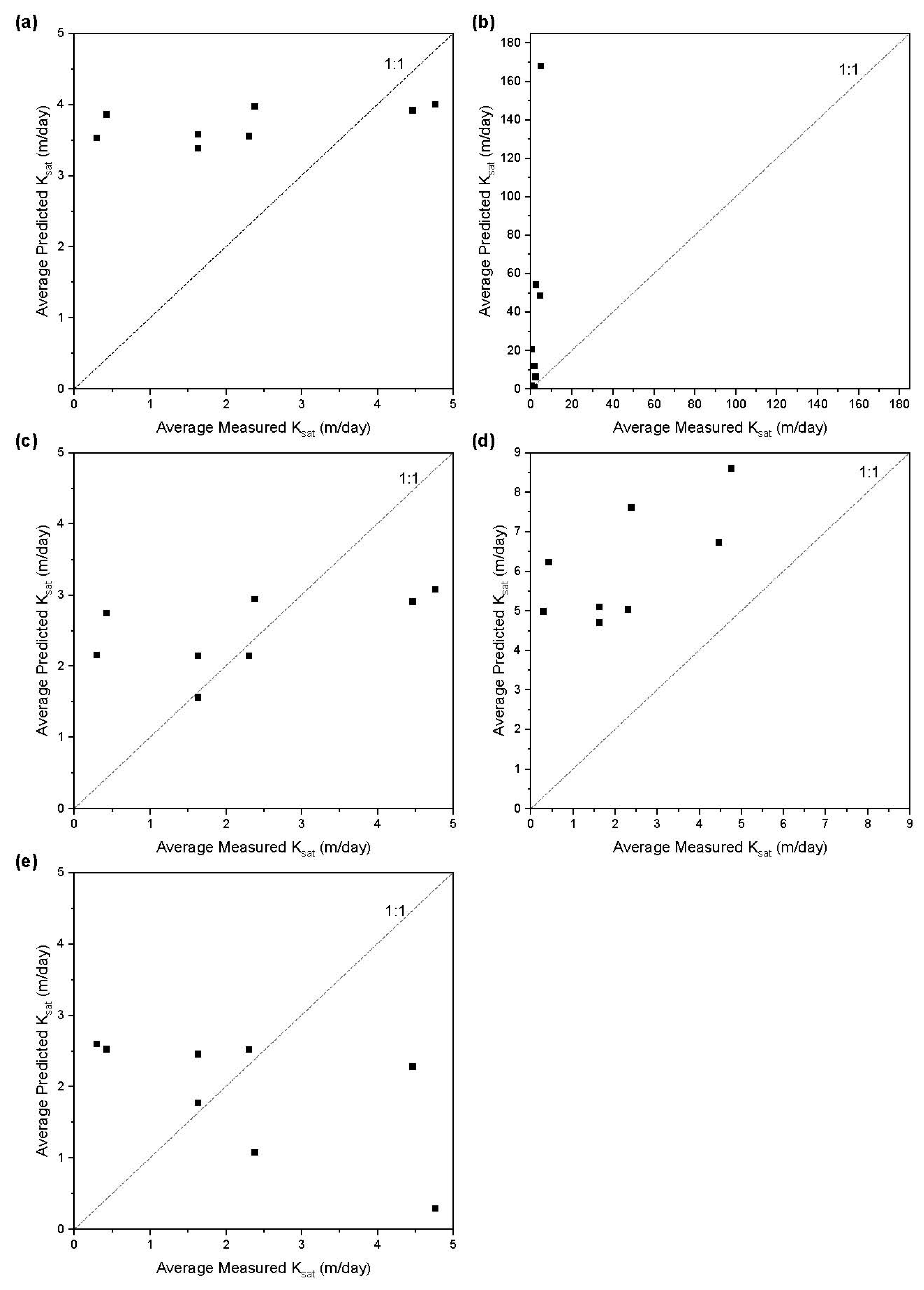
3.5. Model Performance

Model performance is shown in Figure 5 with average predicted K_sat versus averaged measured K_sat at each study site. Four out of five models performed similarly well, as predicted average K_sat were within the same order of magnitude [11,39,40,41]. Predicted K_sat from the Puckett et al. [39] (Figure 5a) and the Smettem and Bristow [41] (Figure 5d) models scattered away from the 1:1 line with most or all values, respectively, falling between the positive y-axis and 1:1 line, representing an overestimation by the models. In contrast, half of the predicted K_sat from the Campbell [40] (Figure 5c) and Saxton et al. [11] models (Figure 5e) scattered along the 1:1 line, indicating smaller relative error and overall better model fits. The Jabro [27] model (Figure 5b) performed poorly, as evidenced by the range of K_sat predictions and distance from the 1:1 line, indicating it was not valid for the RMF soil data. Notably, the Jabro [27] model had the most model parameters (i.e., three) and was the only model to incorporate bdry, indicating that this pedotransfer function was not suited for RMF soils.

The quantified errors for each model are shown in

Table 4. Performance of five site-level soil saturated hydraulic conductivity (K_sat) (m/day) models [11,27,39,40,41] for RMF soil by site and farm-level.

	Puckett et al.		Jabro		Campbell		Smettem and Bristow		Saxton et al.
Site	Error	Squared Error	Error	Squared Error	Error	Squared Error	Error	Squared Error	Error	Squared Error
RMF1	1.25	1.56	3.93	15.45	−0.17	0.03	2.73	7.43	0.21	0.04
RMF2	3.43	11.79	20.29	411.80	2.31	5.36	5.80	33.59	2.09	4.39
RMF3	−0.55	0.30	46.40	2152.97	2.91	8.44	6.73	45.26	2.27	5.18
RMF4	1.59	2.52	51.78	2681.17	0.55	0.30	5.23	27.30	−1.31	1.73
RMF5	−0.76	0.58	163.31	26670.27	−1.69	2.85	3.83	14.69	−4.48	20.04
RMF6	1.75	3.07	−0.60	0.36	−0.07	0.01	3.06	9.38	0.14	0.02
RMF7	1.94	3.78	10.21	104.20	0.51	0.26	3.46	11.96	0.82	0.67
RMF8	3.24	10.47	1.55	2.40	1.86	3.45	4.68	21.93	2.30	5.29
ME		1.49		37.11		0.78		4.44		0.26
SSE		34.07		32038.62		20.68		171.55		37.36
RMSE		2.06		63.28		1.61		4.63		2.16

Note: ME = mean error (m/day); SSE = sum of squared error (m²/day²); RMSE = root of the mean-square error (m/day); unit of error = (m/day); unit of squared error = (m²/day²).

. Farm-level ME for the four validated models ranged from 0.26 m/day with the Saxton et al. [11] model to 4.44 m/day with the Smettem and Bristow [41] model, while the Jabro [27] model ME was 37.11 m/day, which was an order of magnitude larger than the other models. Positive MEs indicate that the models generally overestimated RMF K_sat, but smaller ME values (<1 m/day) for the Saxton et al. [11] and Campbell [40] model confirms better fits to the observed data (Table 4). Error ranges were similar in magnitude (<10) for four of the five models, while the Jabro [27] model error range was two orders of magnitude larger. Similar model error ranges can be partially explained by the variability in the measured K_sat. Although most of the model error ranges were similar, the smaller error ranges for Puckett et al. [39] and Campbell [40] models confirms that they were better fits for the measured data.

3.6. Model Comparison

Similar magnitude farm-level SSE and RMSE for the Puckett et al. [39], Campbell [40], and Saxton et al. [11] models indicates that these models were similar and better fits for the RMF data when compared to the Jabro [27] and Smettem and Bristow [41] models, the estimates from which were characterized by larger SSE and RMSE values (Table 4). SSE ranged from 20.68 m²/m² for the Campbell [40] model to 32038.62 m²/m² for the Jabro [27] model, while RMSE ranged from 1.61 m/day with the Campbell [40] model to 63.28 m/day with the Jabro [27] model (Table 4). The Campbell [40] model was the best fit for the measured data, as it had the smallest farm-level SSE and RMSE, while the Jabro [27] model did not result in a reasonable fit. Additionally, the Campbell [40] model seemed to perform better when the average site-level K_sat were between 1.5 and 2.5 m/day, whereas the other models, did not seem to have a range for better model predictions. The presence of an ideal K_sat range demonstrates that soil-property-based K_sat models could be characterized by an ideal soil texture range, outside of which they become unsuitable. For example, the Saxton et al. [11] model was a better fit for the sandy RMF soils, as it was developed with more sand-dominant textures, while the Jabro [27] model utilized silt-dominant textures and was not accurate for RMF soils. Additionally, the range of soil textures used to develop each model likely influenced the individual model outcomes.

3.7. Model Results Implications

One of the most important implications of the current work is that four out of the five evaluated pedotransfer functions provide a valid, alternative approach to direct K_sat measurements, as evidenced by low ME values (i.e., <4.5 m/day) (Table 4). The similarity in model performance between the Campbell [40] and Saxton et al. [11] models demonstrates their applicability in sand textured soils with similar order of magnitude K_sat. Model predictions were improved with the inclusion of a second particle size parameter, as RMSE for the Campbell [40] and Saxton et al. [11] models decreased, or was similar to the one particle size parameter models (i.e., Puckett et al. [39] and Smettem and Bristow [41]). Although slightly more complicated, two parameter models may provide increased accuracy in K_sat estimates, as in the current work, and therefore may justify additional complexity [98]. The Jabro [27] model, which utilized three model parameters, including bdry, was not a good fit for the measured data, likely due to the RMF soils’ high sand content (average 92%). As such, this applied model comparison shows that particle size based K_sat models provide a good option for practitioners to predict K_sat because (1) gathering the required soil particle size data are relatively simple [36,37,38] and (2) four particle-size-based K_sat models adequately and accurately predicted farm-level K_sat, as evidenced by RMSE < 0.5.

The implications of the current work extend beyond the presentation of measured K_sat and particle size based K_sat model validation. The results increase confidence in K_sat models, especially when observed the data are not readily available. Further application of soil property K_sat models can improve K_sat predictions, and thus understanding of soil–water dynamics, in hydrologic studies throughout the northeast region, Chesapeake Bay Watershed, and areas with readily available particle size data. This model validation work provides practitioners and water resource managers with relatively simple alternatives to easily predict a parameter that is essential for governing shallow groundwater flow, which in turn, can increase K_sat estimate availability and transferability.

4. Conclusions

Soil properties and saturated hydraulic conductivity (K_sat) were measured in a small forested drainage area within the Northeast USA to validate five soil property K_sat models. Soil cores from three sampling depths were collected (n = 179) in a grid design to determine soil characteristics and a series of slug tests were performed to quantify K_sat at eight study sites. Mean dry bulk density (bdry) and porosity ranged from 1.03 to 1.30 g/cm³ and 0.51 to 0.54, respectively. bdry and porosity varied significantly (n = 179; p < 0.05) at the 0–5 cm depth and with study site location, while bdry and porosity were statistically similar at 25–30 and 45–50 cm, indicating that the site soils were homogenous below the surface. On average, soil cores were 92% sand and soil textures were sand or sandy loam. Particle size fractions sites did not differ significantly in average particle size class percentages between soil depths (n = 179; p < 0.05) but did differ significantly by site (n = 8; p < 0.05).

Measured K_sat were 0.35–9.33 m/day and 0.21–4.37 m/day for FH and RH slug tests, respectively, and varied significantly (p < 0.05) with slug test type at three of the eight study sites. Average site K_sat ranged from 0.29 to 4.76 m/day and varied significantly with site (n = 8; p < 0.05). Five pedotransfer functions that predicted K_sat from soil property data were tested. Four models performed well and resulted in low, spatial variability between farm-scale estimated K_sat (CV < 0.5). The models that relied on particle size parameters performed better (RMSE < 4.64 m/day) than the models that relied on particle sizes and bdry (RMSE = 63.26 m/day). Improved K_sat estimates justify using a two-parameter particle size model [40] to predict K_sat at the farm-level for RMF soils.

Study results provide soil property characteristics and demonstrate that using affordable and readily available soil characteristic data can accurately and efficiently predict K_sat. This comparison study validates and supports the use of soil-property-based models to predict K_sat in sandy soils. These results are particularly relevant for understanding regional soil-water dynamics but are also informative for hydrologic studies in landscapes with similar soil properties. The broader impacts of this work extend to providing practitioners with an assessment of K_sat modeling that can used to effectively inform water resource management decisions and increase the applicability of K_sat estimates at locations with available particle size data.

References

1. Qi, S.; Wen, Z.; Lu, C.; Shu, L.; Shao, J.; Huang, Y.; Zhang, S.; Huang, Y. A new empirical model for estimating the hydraulic conductivity of low permeability media. IAHS-AISH Proc. Rep. 2015, 368, 478–483. [Google Scholar] [CrossRef] [Green Version]
2. Hwang, H.T.; Jeen, S.W.; Suleiman, A.A.; Lee, K.K. Comparison of saturated hydraulic conductivity estimated by three different methods. Water (Switzerland) 2017, 9, 942. [Google Scholar] [CrossRef] [Green Version]
3. Freeze, R.A.; Cherry, J.A. Groundwater; Prentice-Hall, Inc.: Englewood Cliffs, NJ, USA, 1979; ISBN 01-336-53129. [Google Scholar]
4. Chapuis, R.P. Predicting the saturated hydraulic conductivity of soils: A review. Bull. Eng. Geol. Environ. 2012, 71, 401–434. [Google Scholar] [CrossRef]
5. Darcy, H. The Public Fountains of the City of Dijon; Dalmont: Paris, France, 1856; ISBN 3663537137. [Google Scholar]
6. Klute, A. Laboratory Measurement of Hydraulic Conductivity of Unsaturated Soil. In Methods of Soil Analysis: Part 1-Physical and Mineralogical Properties, Including Statistics of Measurement and Sampling; Black, C.A., Evans, D.D., White, J.L., Ensminger, L.E., Clark, F.E., Dinauer, R.C., Eds.; American Society of Argronomy: Madison, WI, USA, 1965; pp. 210–221. [Google Scholar]
7. Boersma, L. Field Measurement of Hydraulic Conductivity Above a Water Table. In Methods of Soil Analysis: Part 1-Physical and Mineralogical Properties, Including Statistics of Measurement and Sampling; Black, C.A., Evans, D.D., White, J.L., Ensminger, L.E., Clark, F.E., Dinauer, R.C., Eds.; American Society of Argronomy: Madison, WI, USA, 1965; pp. 222–233. [Google Scholar]
8. Zhang, Y.; Schaap, M.G. Estimation of saturated hydraulic conductivity with pedotransfer functions: A review. J. Hydrol. 2019, 575, 1011–1030. [Google Scholar] [CrossRef]
9. Montzka, C.; Herbst, M.; Weihermüller, L.; Verhoef, A.; Vereecken, H. A global data set of soil hydraulic properties and sub-grid variability of soil water retention and hydraulic conductivity curves. Earth Syst. Sci. Data Discuss. 2017, 1–25. [Google Scholar] [CrossRef] [Green Version]
10. Vereecken, H.; Schnepf, A.; Hopmans, J.W.; Javaux, M.; Or, D.; Roose, T.; Vanderborght, J.; Young, M.H.; Amelung, W.; Aitkenhead, M.; et al. Modeling Soil Processes: Review, Key Challenges, and New Perspectives. Vadose Zone J. 2016, 15, vzj2015.09.0131. [Google Scholar] [CrossRef] [Green Version]
11. Saxton, K.E.; Rawls, W.J.; Romberger, J.S.; Papendick, R. Estimating general soil-water characteristics from texture. Soil Sci. Soc. Am. J. 1986, 5, 1031–1036. [Google Scholar] [CrossRef]
12. Kennedy, C.D.; Murdoch, L.C.; Genereux, D.P.; Corbett, D.R.; Stone, K.; Pham, P.; Mitasova, H. Comparison of Darcian flux calculations and seepage meter measurements in a sandy streambed in North Carolina, United States. Water Resour. Res. 2010, 46, 1–11. [Google Scholar] [CrossRef]
13. Duan, R.; Fedler, C.B.; Borrelli, J. Comparison of methods to estimate saturated hydraulic conductivity in texas soils with grass. J. Irrig. Drain. Eng. 2012, 138, 322–327. [Google Scholar] [CrossRef]
14. Vienken, T.; Dietrich, P. Field evaluation of methods for determining hydraulic conductivity from grain size data. J. Hydrol. 2011, 400, 58–71. [Google Scholar] [CrossRef]
15. Fetter, C.W. Applied Hydrogeology, 4th ed.; Lynch, P., Ed.; Prentice-Hall, Inc.: Upper Saddle River, NJ, USA, 2001; ISBN 9780130882394. [Google Scholar]
16. Reynolds, W.D.; Bowman, B.T.; Brunke, R.R.; Drury, C.F.; Tan, C.S. Comparison of tension infiltrometer, pressure infiltrometer, and soil core estimates of saturated hydraulic conductivity. Soil Sci. Soc. Am. J. 2000, 64, 478–484. [Google Scholar] [CrossRef]
17. Hvorslev, M.J. Time Lag and Soil Permeability in Ground-Water Observations. Waterw. Exp. Station Bull. 1951, 36, 1–55. [Google Scholar]
18. Butler, J.J., Jr. The Design, Performance, and Analysis of Slug Tests; CRC Press LLC: Boca Raton, FL, USA, 1998; ISBN 1-56670-230-5. [Google Scholar]
19. Butler, J.J., Jr.; McElwee, C.D.; Liu, W. Improving the Quality of Parameter Estimates Obtained from Slug Tests. Ground Water 1996, 34, 480–490. [Google Scholar] [CrossRef]
20. Dorsey, J.D.; Ward, A.D.; Fausey, N.R.; Bair, E.S. Comparison of four field methods for measuring saturated hydraulic conductivity. Trans. Am. Soc. Agric. Eng. 1990, 33, 1925–1931. [Google Scholar] [CrossRef]
21. Black, J.H. The practical reasons why slug tests (including falling and rising head tests) often yield the wrong value of hydraulic conductivity. Q. J. Eng. Geol. Hydrogeol. 2010, 43, 345–358. [Google Scholar] [CrossRef]
22. Strayer, D.L.; Beighley, R.E.; Thompson, L.C.; Brooks, S.; Nilsson, C.; Pinay, G.; Naiman, R.J. Effects of land cover on stream ecosystems: Roles of empirical models and scaling issues. Ecosystems 2003, 6, 407–423. [Google Scholar] [CrossRef]
23. Kellner, E.; Hubbart, J.A. Continuous and event-based time series analysis of observed floodplain groundwater flow under contrasting land-use types. Sci. Total Environ. 2016, 566–567, 436–445. [Google Scholar] [CrossRef]
24. Anderson, M.P. Characterization of Geological Heterogeneity; Dagan, G., Neuman, S., Eds.; Cambridge University Press: Cambridge, UK, 1997; ISBN 9780511600081. [Google Scholar]
25. Chen, X.; Song, J.; Wang, W. Spatial variability of specific yield and vertical hydraulic conductivity in a highly permeable alluvial aquifer. J. Hydrol. 2010, 388, 379–388. [Google Scholar] [CrossRef]
26. Van Looy, K.; Bouma, J.; Herbst, M.; Koestel, J.; Minasny, B.; Mishra, U.; Montzka, C.; Nemes, A.; Pachepsky, Y.A.; Padarian, J.; et al. Pedotransfer Functions in Earth System Science: Challenges and Perspectives. Rev. Geophys. 2017, 55, 1199–1256. [Google Scholar] [CrossRef] [Green Version]
27. Jabro, J.D. Estimation of saturated hydraulic conductivity of soils from particle size distribution and bulk density data. Trans. Am. Soc. Agric. Eng. 1992, 35, 557–560. [Google Scholar] [CrossRef]
28. Suleiman, A.A.; Ritchie, J.T. Estimating saturated hydraulic conductivity from soil porosity. Trans. Am. Soc. Agric. Eng. 2001, 44, 235–239. [Google Scholar] [CrossRef]
29. Chapuis, R.P. Predicting the saturated hydraulic conductivity of sand and gravel using effective diameter and void ratio. Can. Geotech. J. 2004, 41, 787–795. [Google Scholar] [CrossRef]
30. Urumović, K. The referential grain size and effective porosity in the Kozeny-Carman model. Hydrol. Earth Syst. Sci. 2016, 20, 1669–1680. [Google Scholar] [CrossRef] [Green Version]
31. Salem, H.S. Application of the Kozeny-Carman equation to permeability determination for a glacial outwash aquifer, using grain-size analysis. Energy Sources 2001, 23, 461–473. [Google Scholar] [CrossRef]
32. Carrier, W.D., III. Goodbye, Hazen; Hello, Kozeny-Carman. J. Geotech. Geoenviron. Eng. 2003, 129, 1054–1056. [Google Scholar] [CrossRef]
33. Carman, P.C. Permeability of saturated sands, soils and clays. J. Agric. Sci. 1939, 29, 262–273. [Google Scholar] [CrossRef]
34. Hazen, A. Some physical properties of sands and gravels, with special reference to their use in filtration. 24th Annu. Rep. 1892, 539–556. [Google Scholar]
35. Kozeny, J. Ueber kapillare Leitung des Wassers im Boden. Wien. Akad. Wiss. 1927, 136, 271. [Google Scholar]
36. Saxton, K.E.; Rawls, W.J. Soil Water Characteristic Estimates by Texture and Organic Matter for Hydrologic Solutions. Soil Sci. Soc. Am. J. 2006, 70, 1569–1578. [Google Scholar] [CrossRef] [Green Version]
37. Hillel, D. Introduction to Environmental Soil Physics; Academic Press: San Diego, CA, USA, 2004; ISBN 0-12-348655-6. [Google Scholar]
38. Vereecken, H.; Maes, J.; Feyen, J. Estimating unsaturated hydraulic conductivity from easily measured soil properties. Soil Sci. 1990, 149, 1–12. [Google Scholar] [CrossRef]
39. Puckett, W.E.; Dane, J.H.; Hajek, B. Physical and Mineralogical Data to Determine Soil Hydraulic Properties†. Soil Sci. Soc. Am. J. 1985, 49, 831–836. [Google Scholar] [CrossRef]
40. Campbell, G.S. Soil Physics with BASIC: Transport Models for Soil-Plant Systems; Elsevier Scientific: New York, NY, USA, 1985. [Google Scholar]
41. Smettem, K.R.J.; Bristow, K.L. Obtaining soil hydraulic properties for water balance and leaching models from survey data. 2. Hydraulic conductivity. Aust. J. Agric. Res. 1999, 50, 1259–1262. [Google Scholar] [CrossRef]
42. Schaap, M.G.; Leij, F.J.; van Genuchten, M.T. ROSETTA: A computer program for estimating soil hydraulic parameters with hierarchical pedotransfer functions. J. Hydrol. 2002, 251, 163–176. [Google Scholar] [CrossRef]
43. Decharme, B.; Douville, H.; Boone, A.; Habets, F.; Noilhan, J. Impact of an exponential profile of saturated hydraulic conductivity within the ISBA LSM: Simulations over the Rhône basin. J. Hydrometeorol. 2006, 7, 61–80. [Google Scholar] [CrossRef] [Green Version]
44. Maest, A.; Kuipers, J.R.; Travers, C.L.; Atkins, D.A. Predicting Water Quality at Hardrock Mines: Methods and Models, Uncertainties, and State-of-the Art; Kuipers & Associates: Butte, MT, USA, 2005.
45. United States Army Corps of Engineers. Hydrologic Modeling System HEC-HMS Technical Reference Manual. 2000. Available online: https://www.hec.usace.army.mil/software/hec-hms/documentation/HEC-HMS_Technical%20Reference%20Manual_(CPD-74B).pdf (accessed on 2 April 2020).
46. Chapuis, R.P.; Dallaire, V.; Marcotte, D.; Chouteau, M.; Acevedo, N.; Gagnon, F. Evaluating the hydraulic conductivity at three different scales within an unconfined sand aquifer at Lachenaie, Quebec. Can. Geotech. J. 2005, 42, 1212–1220. [Google Scholar] [CrossRef]
47. Harbaugh Arlen, W. MODFLOW-2005, The U.S. Geological Survey Modular Ground-Water Model—The Ground-Water Flow Process. USGS 2005. [Google Scholar] [CrossRef] [Green Version]
48. Roberts, T.; Lazarovitch, N.; Warrick, A.W.; Thompson, T.L. Modeling Salt Accumulation with Subsurface Drip Irrigation Using HYDRUS-2D. Soil Sci. Soc. Am. J. 2009, 73, 233–240. [Google Scholar] [CrossRef]
49. Ortoleva, P.; Merino, E.; Moore, C.; Chadam, J. Geochemical self-organization in reaction-transport feedbacks and modelling approach. Am. J. Sci. 1987, 287, 979–1007. [Google Scholar] [CrossRef]
50. Li, Y.; Zhang, Q.; Lu, J.; Yao, J.; Tan, Z. Assessing surface water–groundwater interactions in a complex river-floodplain wetland-isolated lake system. River Res. Appl. 2019, 35, 25–36. [Google Scholar] [CrossRef] [Green Version]
51. Lin, Y.-C.; Medina, M.A., Jr. Incorporating transient storage in conjunctive stream–aquifer modeling. Adv. Water Resour. 2003, 26, 1001–1019. [Google Scholar] [CrossRef]
52. Hubbart, J.A.; Holmes, J.; Bowman, G. TMDLs: Improving Stakeholder Acceptance with Science-based Allocations. Watershed Sci. Bull. 2010, 1, 19–24. [Google Scholar]
53. Hubbart, J.A.; Kellner, E.; Zeiger, S.J. A case-study application of the experimental watershed study design to advance adaptive management of contemporary watersheds. Water 2019, 11, 2355. [Google Scholar] [CrossRef] [Green Version]
54. Nichols, J.; Hubbart, J.A.; Poulton, B.C. Using macroinvertebrate assemblages and multiple stressors to infer urban stream system condition: A case study in the central US. Urban. Ecosyst. 2016, 19, 679–704. [Google Scholar] [CrossRef]
55. Zeiger, S.J.; Hubbart, J.A. Quantifying suspended sediment flux in a mixed-land-use urbanizing watershed using a nested-scale study design. Sci. Total Environ. 2016, 542, 315–323. [Google Scholar] [CrossRef] [PubMed]
56. Tetzlaff, D.; Carey, S.K.; Mcnamara, J.P.; Laudon, H.; Soulsby, C. The essential value of long-term experimental data for hydrology and water management. Water Resour. Res. 2017, 53, 2598–2604. [Google Scholar] [CrossRef] [Green Version]
57. Zell, C.; Kellner, E.; Hubbart, J.A. Forested and agricultural land use impacts on subsurface floodplain storage capacity using coupled vadose zone-saturated zone modeling. Environ. Earth Sci. 2015, 74, 7215–7228. [Google Scholar] [CrossRef]
58. Gellis, A.C.; Hupp, C.R.; Pavich, M.J.; Landwehr, J.M.; Banks, W.S.L.; Hubbard, B.E.; Landland, M.J.; Ritchie, J.C.; Reuter, J.M. Sources, Transport, and Storage of Sediment at Selected Sites in the Chesapeake Bay Watershed. USGS 2009. [Google Scholar] [CrossRef]
59. Zhang, Q.; Blomquist, J.D. Watershed export of fine sediment, organic carbon, and chlorophyll-a to Chesapeake Bay: Spatial and temporal patterns in 1984–2016. Sci. Total Environ. 2018, 619–620, 1066–1078. [Google Scholar] [CrossRef]
60. Boesch, D.F.; Greer, J. Chesapeake Futures: Choices for the 21st Century; Scientific and Technical Advisory Committee: Edgewater, MD, USA, 2003; p. 160. [Google Scholar]
61. Natural Resource Analysis Center at West Virginia University. WV Land Use Land Cover (NAIP 2016). Available online: http://wvgis.wvu.edu/data/dataset.php?ID=489 (accessed on 15 February 2020).
62. WV GIS Technical Center. Digital Elevation Model 1- to 3-Meter Statewide Mosaic. Available online: http://wvgis.wvu.edu/data/dataset.php?ID=477 (accessed on 2 September 2019).
63. Soil Survey Staff, Natural Resources Conservation Service, United States Department of Agriculture. Web Soil Survey. Available online: https://websoilsurvey.sc.egov.usda.gov/ (accessed on 28 February 2020).
64. Knight, H.G. Reymann Memorial Farms. W. Va. Agric. For. Exp. Station Bull. 1925, 194, 1–20. [Google Scholar]
65. Estepp, R. Soil Survey of Grant and Hardy Counties West Virginia; United States Department of Agriculture: Washington, DC, USA, 1989.
66. Smith, R.M.; Pohlman, G.G.; Browning, D.R. Some Soil Properties which Influence the Use of Land in West Virginia. W. Va. Agric. For. Exp. Station Bull. 1945, 321, 1–71. [Google Scholar]
67. Natural Resources Conservation Service (NRCS) Web Site for Official Soil Series Descriptions and Series Classification. Available online: https://soilseries.sc.egov.usda.gov/ (accessed on 13 February 2020).
68. Dean, S.L.; Lessing, P.; Kulander, B.R. Geology of the Rio Quadrangle, Hampshire and Hardy Counties; OF-0004; West Virginia Geological and Economic Survey Open File Publication: Morgantown, WV, USA, 1999. [Google Scholar]
69. Horton, J.D.; San Juan, C.A.; Stoeser, D.B. The State Geologic Map Compilation (SGMC) geodatabase of the conterminous United States (ver. 1.1, August 2017). In U.S. Geological Survey Data Series 1052; U.S. Geological Survey: Reston, VA, USA, 2017; p. 46. [Google Scholar]
70. Kellner, E.; Hubbart, J. Agricultural and forested land use impacts on floodplain shallow groundwater temperature regime. Hydrol. Process. 2015, 30, 625–636. [Google Scholar] [CrossRef]
71. Zeiger, S.J.; Hubbart, J.A. Urban stormwater temperature surges: A central US watershed study. Hydrology 2015, 2, 193–209. [Google Scholar] [CrossRef]
72. Hubbart, J.A.; Link, T.E.; Gravelle, J.A.; Elliot, W.J. Timber harvest impacts on water yield in the continental/maritime hydroclimatic region of the United States. For. Sci. 2007, 53, 169–180. [Google Scholar] [CrossRef]
73. National Oceanic and Atmospheric Administration (NOAA) Climate Data Online Search. Available online: https://www.ncdc.noaa.gov/cdo-web/search (accessed on 20 April 2020).
74. Blake, G.R. Bulk Density. In Methods of Soil Analysis: Part 1-Physical and Mineralogical Properties, Including Statistics of Measurement and Sampling; Black, C.A., Evans, D.D., White, J.L., Ensminger, L.E., Clark, F.E., Dinauer, R.C., Eds.; American Society of Agronomy: Madison, WI, USA, 1965; pp. 374–390. [Google Scholar]
75. Hubbart, J.A.; Muzika, R.-M.; Dandan, H.; Robinson, A. Bottomland Hardwood Forest Influence on Soil Water Consumption in an Urban floodplain: Potential To Improve Flood Storage Capacity and Reduce Stormwater Runoff. Watershed Sci. Bull. 2011, 2, 34–43. [Google Scholar]
76. Vomocil, J.A. Porosity. In Methods of Soil Analysis: Part 1-Physical and Mineralogical Properties, Including Statistics of Measurement and Sampling; Black, C.A., Evans, D.D., White, J.L., Ensminger, L.E., Clark, F.E., Dinauer, R.C., Eds.; American Society of Agronomy: Madison, WI, USA, 1965; pp. 299–314. [Google Scholar]
77. Hoffmann, C.C.; Berg, P.; Dahl, M.; Larsen, S.E.; Andersen, H.E.; Andersen, B. Groundwater flow and transport of nutrients through a riparian meadow—Field data and modelling. J. Hydrol. 2006, 331, 315–335. [Google Scholar] [CrossRef]
78. Davis, J.C. Statistics and Data Analysis in Geology, 3rd ed.; J. Wiley: New York, NY, USA, 2002; ISBN 0471172758 9780471172758. [Google Scholar]
79. Gordon, N.D.; McMahon, T.A.; Finlayson, B.L.; Gippel, C.J.; Nathan, R.J. Stream Hydrology: An Introduction for Ecologists, 2nd ed.; J. Wiley: New York, NY, USA, 2004; ISBN 978-0-470-84358-1. [Google Scholar]
80. Skinner, J. A study of the methods used in measurement and analysis of sediment loads in reservoirs. In Report NN; Federal Interagency Sedimentation Project: Vicksburg, MS, USA, 2000. [Google Scholar]
81. Gee, G.W.; Or, D. Particle-Size Analysis. Methods of soil analysis. Part 4. In Methods of Soil Analysis, Part 4, Phyiscal Methods; Dane, J.H., Topp, G.C., Eds.; ACSESS: Madison, WI, USA, 2002; pp. 255–293. ISBN 978-0-89118-893-3. [Google Scholar]
82. Soil Survey Staff. Soil Taxonomy: A Basic System of Soil Classification for Making and Interpreting Soil Surveys, 2nd ed.; Natural Resources Conservation Service: Washington, DC, USA, 1999.
83. Nemes, A.; Rawls, W.J. Soil texture and particle-size distribution as input to estimate soil hydraulic properties. In Developments in Soil Science; Pachepsky, Y., Rawls, W.J., Eds.; Elsevier Science: Amsterdam, The Netherlands, 2004; Volume 30, pp. 47–70. [Google Scholar]
84. Song, J.; Chen, X.; Cheng, C.; Wang, D.; Lackey, S.; Xu, Z. Feasibility of grain-size analysis methods for determination of vertical hydraulic conductivity of streambeds. J. Hydrol. 2009, 375, 428–437. [Google Scholar] [CrossRef]
85. Day, P.R. Particle Fractionation and Particle-Size Analysis. In Methods of Soil Analysis: Part 1 Physical and Mineralogical Properties, Including Statistics of Measurement and Sampling; Black, C.A., Evans, D.D., White, J.L., Ensminger, L.E., Clark, F.E., Dinauer, R.C., Eds.; American Society of Agronomy: Madison, WI, USA, 1965; pp. 545–567. [Google Scholar]
86. 2540 Solids (2017). Standard Methods for the Examination of Water and Wastewater, 23rd. Available online: https://www.standardmethods.org/doi/abs/10.2105/SMWW.2882.030 (accessed on 2 March 2020).
87. Kettler, T.A.; Doran, J.W.; Gilbert, T.L. Simplified Method for Soil Particle-Size Determination to Accompany Soil-Quality Analyses. Soil Biol. Biochem. 2001, 65, 849–852. [Google Scholar] [CrossRef] [Green Version]
88. Natural Resources Conservation Service (NRCS) Soil Texture Calculator. Available online: http://soils.usda.gov/technical/aids/investigations/texture/%5Cnhttp://www.nrcs.usda.gov/wps/portal/nrcs/detail/soils/survey/?cid=nrcs142p2_054167 (accessed on 15 April 2020).
89. Solinst Canada, Ltd. Available online: https://www.solinst.com/products/dataloggers-and-telemetry/3001-levelogger-series/operating-instructions/user-guide/1-introduction/1-1-1-levelogger-edge.php (accessed on 6 February 2020).
90. Cheong, J.Y.; Hamm, S.Y.; Kim, H.S.; Ko, E.J.; Yang, K.; Lee, J.H. Estimating hydraulic conductivity using grain-size analyses, aquifer tests, and numerical modeling in a riverside alluvial system in South Korea. Hydrogeol. J. 2008, 16, 1129–1143. [Google Scholar] [CrossRef]
91. Barbour, M.G.; Burk, J.H.; Pitts, W.D.; Gilliam, F.S.; Schwartz, M.W. Terrestrial Plant Ecology, 3rd ed.; Addison Wesley Longman: Menlo Park, CA, USA, 1999; ISBN 080530004X. [Google Scholar]
92. Hall, D.G.M.; Reeve, M.J.; Thomasson, A.J.; Wright, V.F. Water Retention, Porosity and Density of Field Soils; Rothamsted Experimental Station: Harpenden, UK, 1977. [Google Scholar]
93. Rai, R.K.; Singh, V.P.; Upadhyay, A. Soil Analysis. In Planning and Evaluation of Irrigation Projects: Methods and Implementation; Maragioglio, N., Ed.; Academic Press: London, UK, 2017; p. 678. ISBN 9780128117484. [Google Scholar]
94. Nimmo, J.R. Porosity and Pore-Size Distribution. Encycl. Soils Environ. 2004, 4, 295–303. [Google Scholar] [CrossRef]
95. McElwee, C.D. Improving the analysis of slug tests. J. Hydrol. 2002, 269, 122–133. [Google Scholar] [CrossRef]
96. Stanford, K.L.; McElwee, C.D. Analyzing slug tests in wells screened across the watertable: A field assessment. Nat. Resour. Res. 2000, 9, 111–124. [Google Scholar] [CrossRef]
97. Soil Survey Staff. Soil Survey Field and Laboratory Methods Manual. Soils Survey Investigations Report No. 51, Version 2.0; Burt, R., Soil Survey Staff, Eds.; United States Department of Agriculture, Natural Resources Conservation Service: Washington, DC, USA, 2014; ISBN 978-0359573516.
98. Lees, M.J. Data-based mechanistic modelling and forecasting of hydrological systems. J. Hydroinf. 2000, 2, 15–34. [Google Scholar] [CrossRef] [Green Version]
Figure 1. (a) The location of Reymann Memorial Farm within the upper Chesapeake Bay Watershed and (b) the locations of eight co-located, nested piezometers throughout the Moore’s Run drainage area, Wardensville, West Virginia, USA [61,62]. (c) Soil core grid design of the current study in Wardensville, West Virginia, USA. SW represents an example stilling well location and P represents an example piezometer location in relation to Moore’s Run. The dashed arrow indicates the flow direction towards the Cacapon River.
Water 12 02040 g001
Figure 2. Soil dry bulk density (g/cm3) (a) and porosity (b) for all sites, by depth throughout the Moore’s Run Watershed, Wardensville, West Virginia, USA. Boxes define the interquartile range (IQR). Vertical lines show the range within 1.5 IQR. Midlines indicate the median. Circles within the boxes denote the mean. Filled-in points indicate potential outliers.
Water 12 02040 g002
Figure 3. Particle size fractions including Sand (a), Silt (b), and Clay (c) for all sites, by depth throughout the Moore’s Run Watershed, Wardensville, West Virginia, USA. Note that the axis ranges differ for each particle size fraction. Boxes define the interquartile range (IQR). Vertical lines show the range within 1.5 IQR. Midlines indicate the median. Circles within the boxes denote the mean. Filled-in points indicate potential outliers. Note the differences in y-axis ranges.
Water 12 02040 g003
Figure 4. Bar plots of average soil saturated hydraulic conductivity (Ksat) (m/day) at eight study sites derived from falling head (left hand bar) and rising head (right hand bar) slug tests during the study period (September 2019–March 2020), Wardensville, West Virginia, USA. Box heights denote the mean value. Vertical lines define the standard deviation. Asterisks denote significant differences (p < 0.05) between the falling head and rising head derived average Ksat values.
Water 12 02040 g004
Figure 5. (a) Puckett et al. [39] model, (b) Jabro [27] model, (c) Campbell [40], (d) Smettem and Bristow [41], and (e) Saxton et al. [11] model predicted soil saturated hydraulic conductivity (Ksat) (m/day) versus measured values at Reymann Memorial Farm.
Water 12 02040 g005