Susceptibility Mapping of Soil Water Erosion Using Machine Learning Models

 ,
, 
 ,
,
Abstract
1. Introduction
2. Materials and Methods
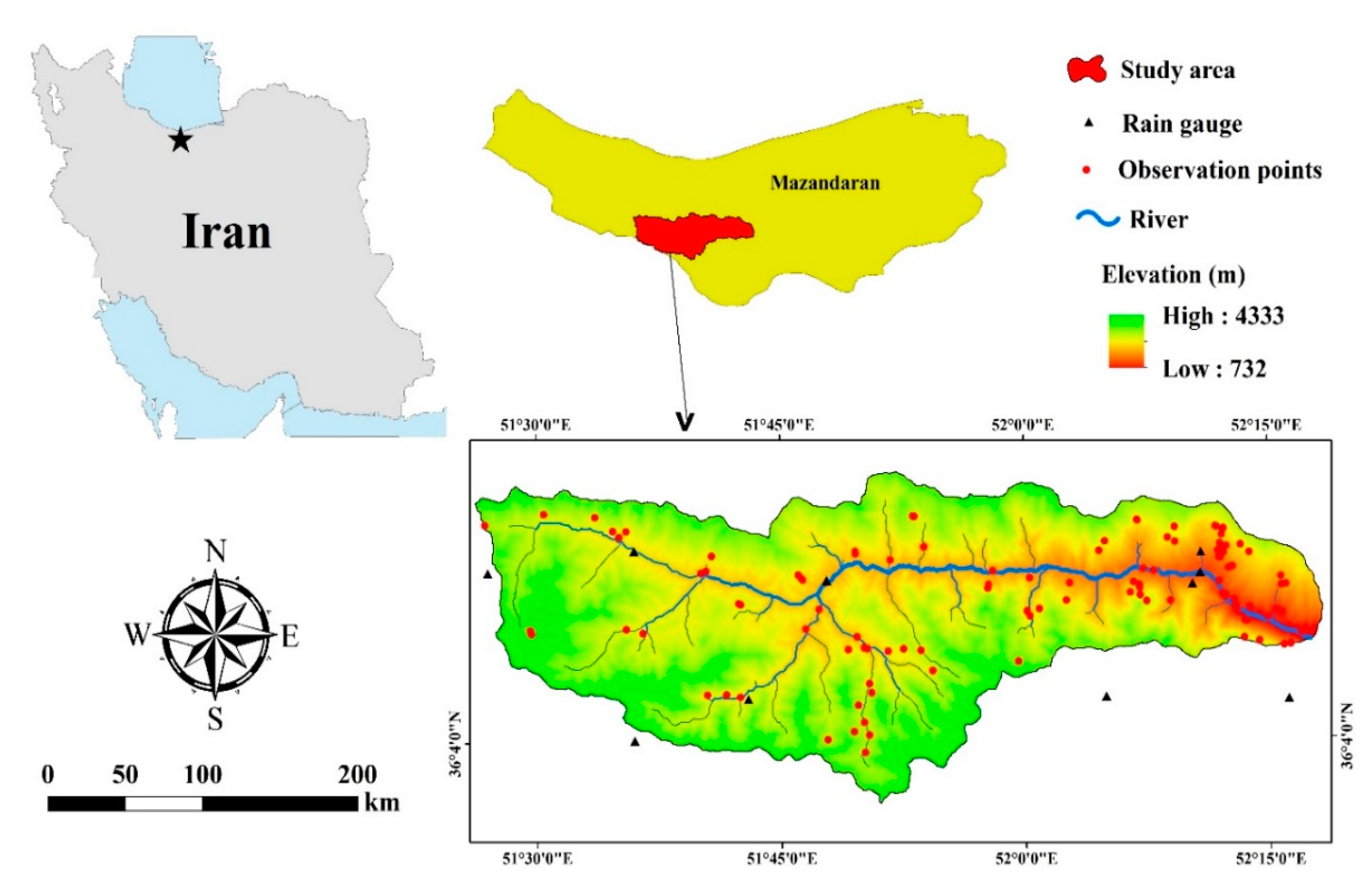
2.1. Study Area
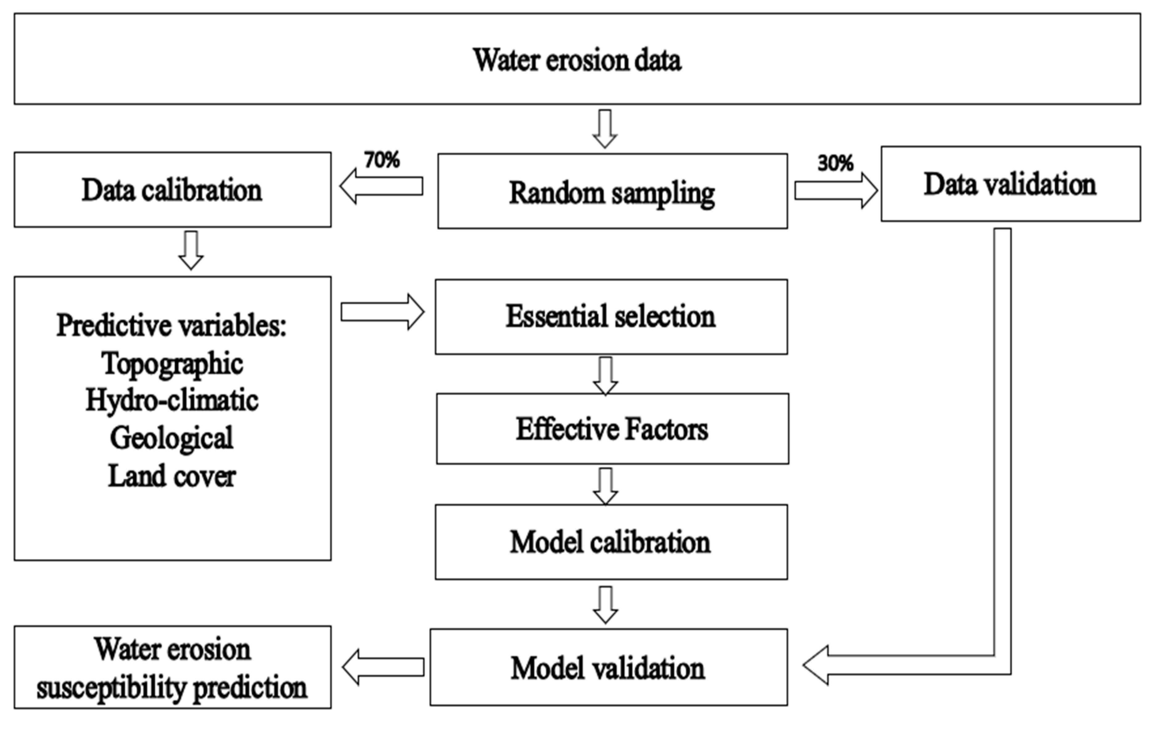
2.2. Methodology
2.2.1. Field Data
2.2.2. Predictive Variables
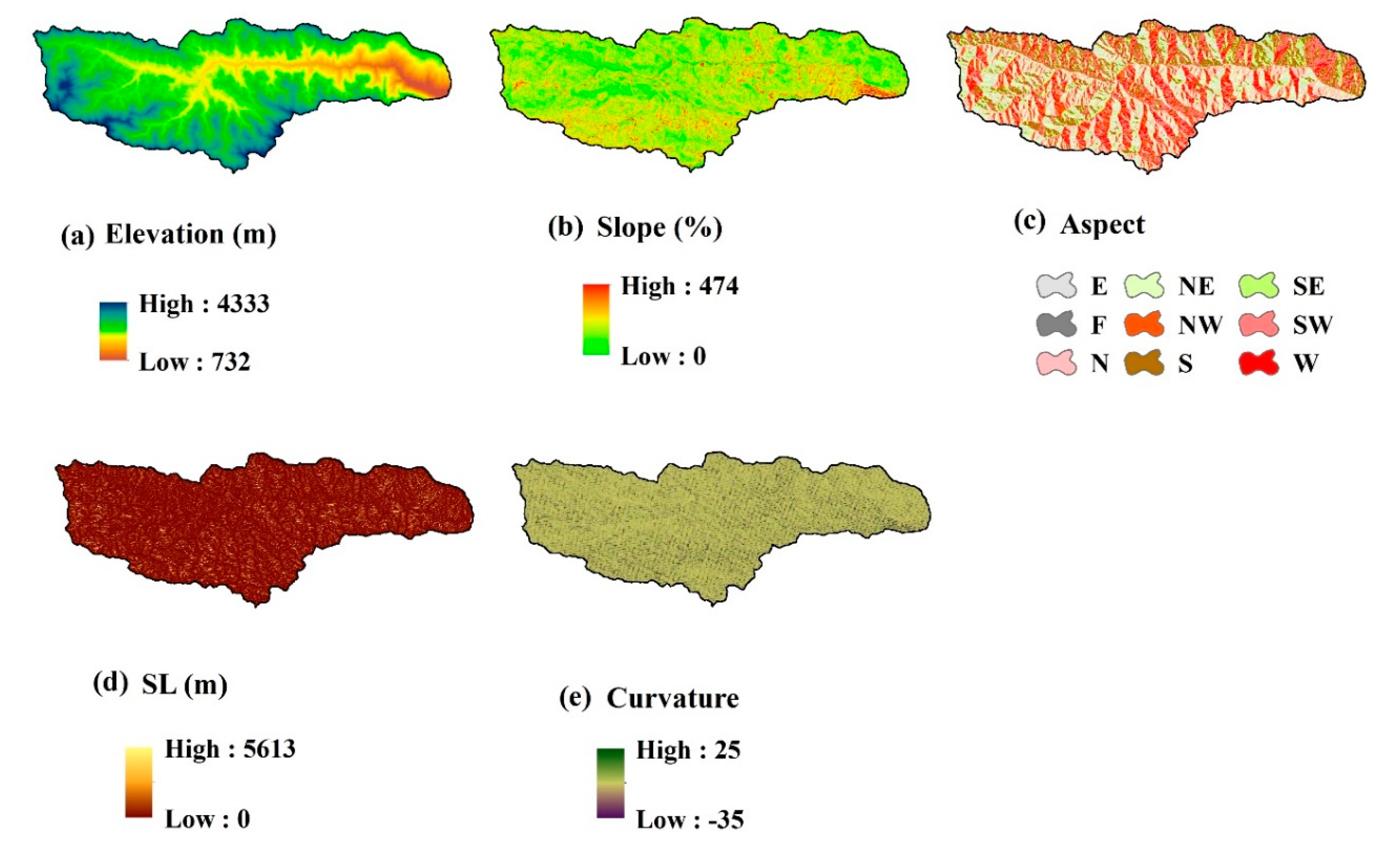
Topographic Parameters
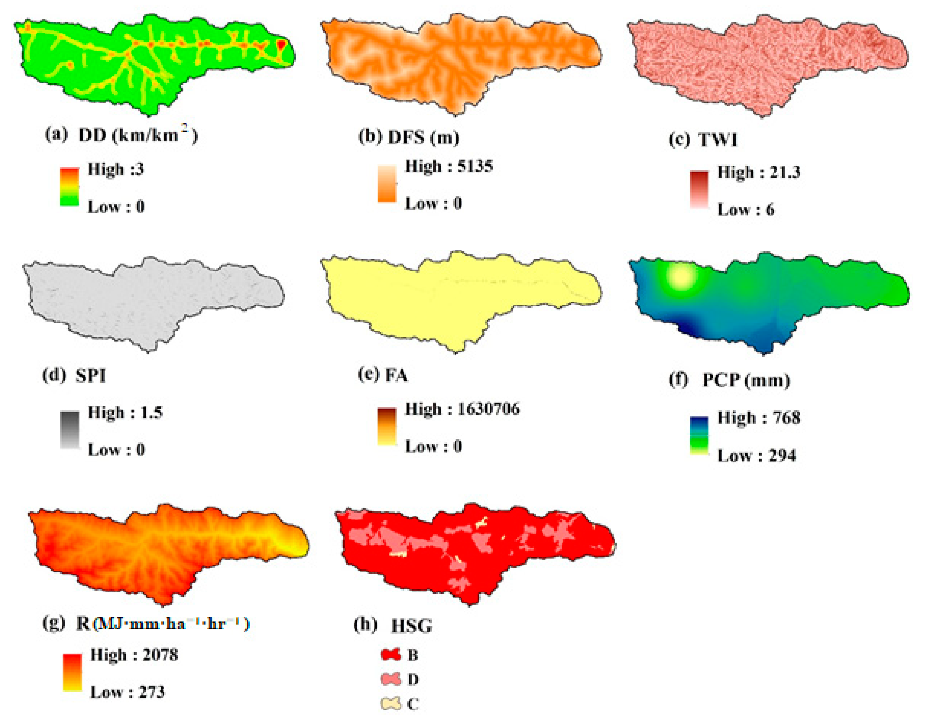
Hydro-Climate Factors
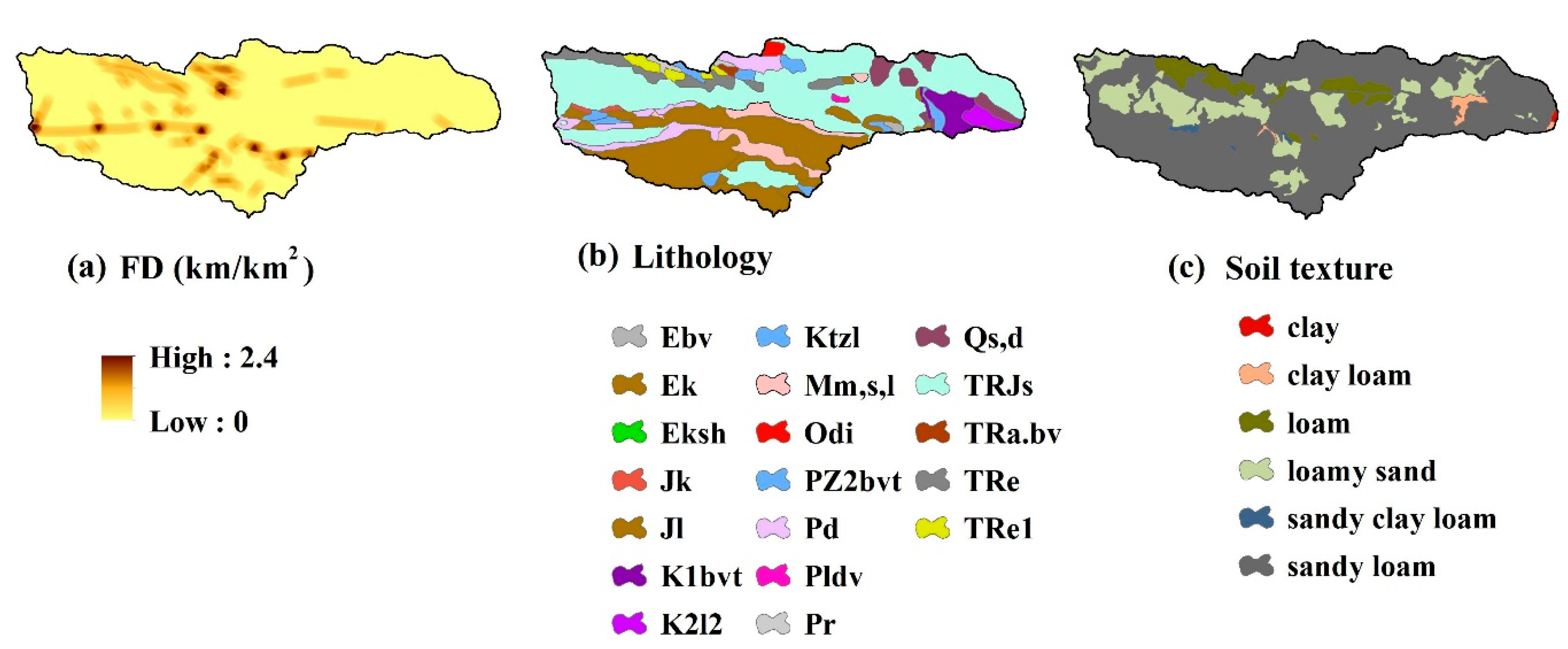
Geological Factors
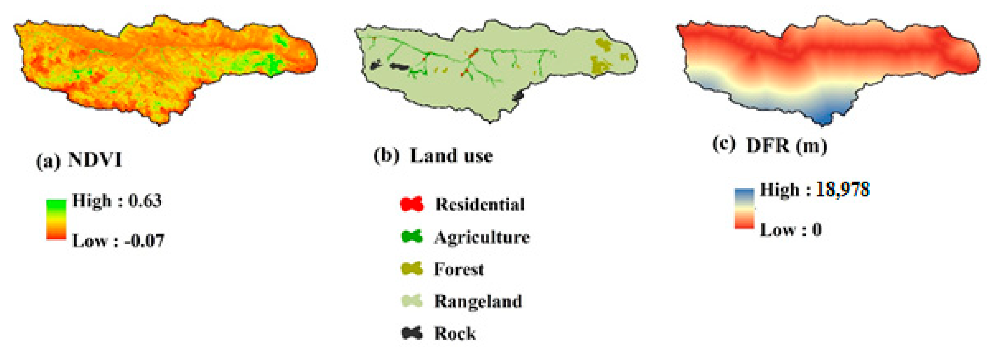
Land Cover Factors
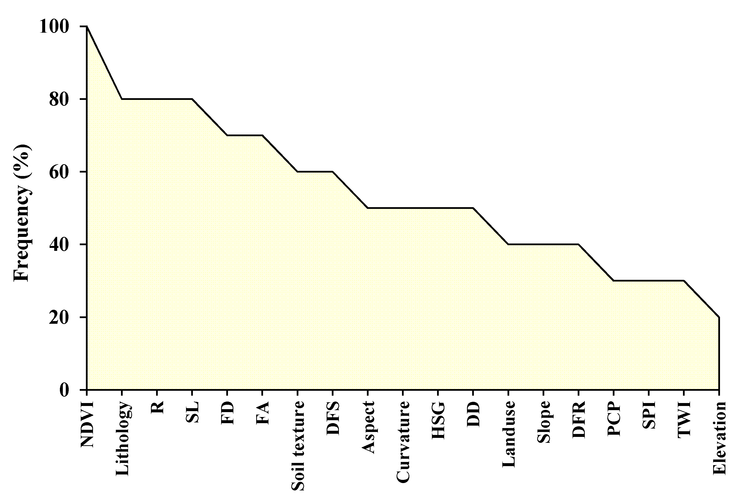
2.2.3. Feature Selection
2.2.4. Weighted Subspace Random Forest (WSRF)
2.2.5. Naive Bayes (NB)
- A response vector, which includes the value of the class variable.
- The feature matrix, which includes all the rows of the dataset and each row contains all the dependent features.
2.2.6. The Gaussian Process with a Radial Basis Function Kernel (Gaussprradial)
2.2.7. Model Calibration and Validation
3. Results and Discussion
3.1. Feature Selection Results
3.2. Results of Water Erosion Modeling
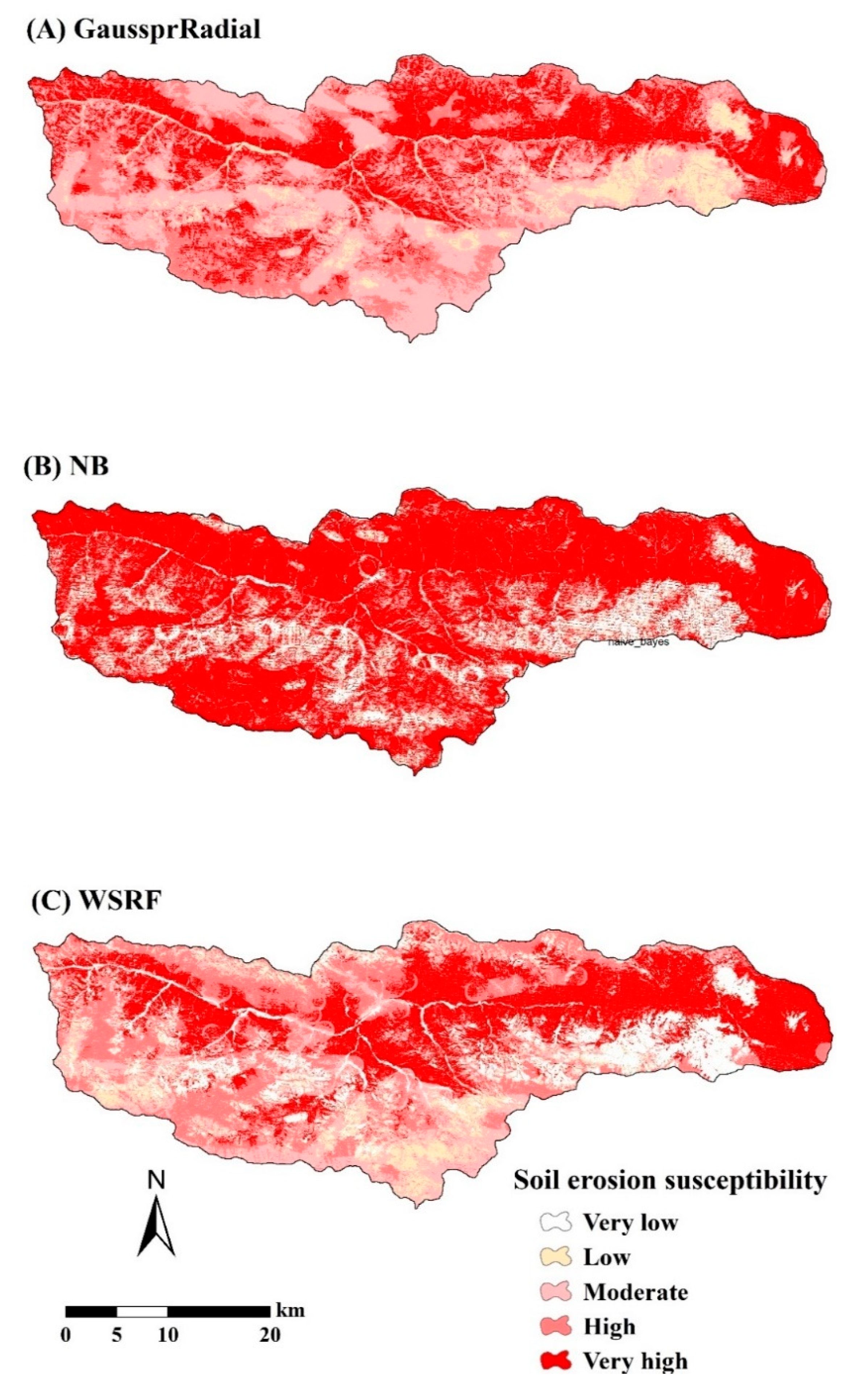
3.3. Spatial Prediction of Water Erosion Susceptibility
4. Conclusions
Author Contributions
Funding
Conflicts of Interest
References
- Morgan, R.P.C. Soil Erosion and Conservation; John Wiley & Sons: Hoboken, NJ, USA, 2005; ISBN 9788578110796. [Google Scholar]
- Vanmaercke, M.; Poesen, J.; Verstraeten, G.; de Vente, J.; Ocakoglu, F. Sediment yield in Europe: Spatial patterns and scale dependency. Geomorphology 2011, 130, 142–161. [Google Scholar] [CrossRef]
- Panagos, P.; Borrelli, P.; Meusburger, K.; Alewell, C.; Lugato, E.; Montanarella, L. Estimating the soil erosion cover-management factor at the European scale. Land Use Policy 2015, 48, 38–50. [Google Scholar] [CrossRef]
- García-Ruiz, J.M.; Beguería, S.; Lana-Renault, N.; Nadal-Romero, E.; Cerdà, A. Ongoing and Emerging Questions in Water Erosion Studies. Land Degrad. Dev. 2017, 28, 5–21. [Google Scholar] [CrossRef]
- Scott, A. Water Erosion in the Murray-Darling Basin: Learning from the Past; Elsevier: New York, NY, USA, 2001. [Google Scholar]
- Sharma, A.; Tiwari, K.N.; Bhadoria, P.B.S. Effect of land use land cover change on soil erosion potential in an agricultural watershed. Environ. Monit. Assess. 2011, 173, 789–801. [Google Scholar] [CrossRef]
- Alkharabsheh, M.M.; Alexandridis, T.K.; Bilas, G.; Misopolinos, N.; Silleos, N. Impact of Land Cover Change on Soil Erosion Hazard in Northern Jordan Using Remote Sensing and GIS. Procedia Environ. Sci. 2013, 19, 912–921. [Google Scholar] [CrossRef]
- Sajedi-Hosseini, F.; Choubin, B.; Solaimani, K.; Cerdà, A.; Kavian, A. Spatial prediction of soil erosion susceptibility using a fuzzy analytical network process: Application of the fuzzy decision making trial and evaluation laboratory approach. Land Degrad. Dev. 2018, 29, 3092–3103. [Google Scholar] [CrossRef]
- Md. Rejaur, R.; Shi, Z.H.; Chongfa, C. Land use/land cover change analysis using geo- information technology: Two case studies in Bangladesh and China. Int. J. Geoinformatics 2009, 5, 25–37. [Google Scholar]
- Vaezi, A.R.; Abbasi, M.; Bussi, G.; Keesstra, S. Modeling Sediment Yield in Semi-Arid Pasture Micro-Catchments, NW Iran. Land Degrad. Dev. 2017, 28, 1274–1286. [Google Scholar] [CrossRef]
- Afshar, F.A.; Ayoubi, S.; Jalalian, A. Soil redistribution rate and its relationship with soil organic carbon and total nitrogen using 137Cs technique in a cultivated complex hillslope in western Iran. J. Environ. Radioact. 2010, 101, 606–614. [Google Scholar] [CrossRef]
- Khalili Moghadam, B.; Jabarifar, M.; Bagheri, M.; Shahbazi, E. Effects of land use change on soil splash erosion in the semi-arid region of Iran. Geoderma 2015, 241, 210–220. [Google Scholar] [CrossRef]
- Pradeep, G.S.; Krishnan, M.V.N.; Vijith, H. Identification of critical soil erosion prone areas and annual average soil loss in an upland agricultural watershed of Western Ghats, using analytical hierarchy process (AHP) and RUSLE techniques. Arab. J. Geosci. 2015, 8, 3697–3711. [Google Scholar] [CrossRef]
- Choubin, B.; Rahmati, O.; Tahmasebipour, N.; Feizizadeh, B.; Pourghasemi, H.R. Application of fuzzy analytical network process model for analyzing the gully erosion susceptibility. Adv. Nat. Technol. Hazards Res. 2019, 48, 105–125. [Google Scholar] [CrossRef]
- Angileri, S.E.; Conoscenti, C.; Hochschild, V.; Märker, M.; Rotigliano, E.; Agnesi, V. Water erosion susceptibility mapping by applying Stochastic Gradient Treeboost to the Imera Meridionale River Basin (Sicily, Italy). Geomorphology 2016, 262, 61–76. [Google Scholar] [CrossRef]
- Svoray, T.; Michailov, E.; Cohen, A.; Rokah, L.; Sturm, A. Predicting gully initiation: Comparing data mining techniques, analytical hierarchy processes and the topographic threshold. Earth Surf. Process. Landf. 2012, 37, 607–619. [Google Scholar] [CrossRef]
- Lee, S.; Ryu, J.H.; Lee, M.J.; Won, J.S. Use of an artificial neural network for analysis of the susceptibility to landslides at Boun, Korea. Environ. Geol. 2003, 44, 820–833. [Google Scholar] [CrossRef]
- Pourghasemi, H.R.; Rossi, M. Landslide susceptibility modeling in a landslide prone area in Mazandarn Province, north of Iran: A comparison between GLM, GAM, MARS, and M-AHP methods. Theor. Appl. Climatol. 2017, 130, 609–633. [Google Scholar] [CrossRef]
- Pradhan, B. A comparative study on the predictive ability of the decision tree, support vector machine and neuro-fuzzy models in landslide susceptibility mapping using GIS. Comput. Geosci. 2013, 51, 350–365. [Google Scholar] [CrossRef]
- Taner San, B. An evaluation of SVM using polygon-based random sampling inlandslide susceptibility mapping: The Candir catchment area(western Antalya, Turkey). Int. J. Appl. Earth Obs. Geoinf. 2014, 26, 399–412. [Google Scholar] [CrossRef]
- Dou, J.; Yamagishi, H.; Pourghasemi, H.R.; Yunus, A.P.; Song, X.; Xu, Y.; Zhu, Z. An integrated artificial neural network model for the landslide susceptibility assessment of Osado Island, Japan. Nat. Hazards 2015, 78, 1749–1776. [Google Scholar] [CrossRef]
- Gorsevski, P.V.; Brown, M.K.; Panter, K.; Onasch, C.M.; Simic, A.; Snyder, J. Landslide detection and susceptibility mapping using LiDAR and an artificial neural network approach: A case study in the Cuyahoga Valley National Park, Ohio. Landslides 2016, 13, 467–484. [Google Scholar] [CrossRef]
- Hong, H.; Pourghasemi, H.R.; Pourtaghi, Z.S. Landslide susceptibility assessment in Lianhua County (China): A comparison between a random forest data mining technique and bivariate and multivariate statistical models. Geomorphology 2016, 259, 105–118. [Google Scholar] [CrossRef]
- Yuan, L.; Zhang, Q.; Li, W.; Zou, L. Debris Flow Hazard Assessment Based on Support Vector Machine. In 2006 IEEE International Symposium on Geoscience and Remote Sensing; IEEE: Piscataway, NJ, USA, 2006; Volume 11, pp. 4221–4224. [Google Scholar]
- Chang, T.C. Risk degree of debris flow applying neural networks. Nat. Hazards 2007, 42, 209–224. [Google Scholar] [CrossRef]
- Chang, T.C.; Chao, R.J. Application of back-propagation networks in debris flow prediction. Eng. Geol. 2006, 85, 270–280. [Google Scholar] [CrossRef]
- Eustace, A.H.; Pringle, M.J.; Denham, R.J. A risk map for gully locations in central Queensland, Australia. Eur. J. Soil Sci. 2011, 62, 431–441. [Google Scholar] [CrossRef]
- Rahmati, O.; Tahmasebipour, N.; Haghizadeh, A.; Pourghasemi, H.R.; Feizizadeh, B. Evaluation of different machine learning models for predicting and mapping the susceptibility of gully erosion. Geomorphology 2017, 298, 118–137. [Google Scholar] [CrossRef]
- Arabameri, A.; Rezaei, K.; Cerda, A.; Lombardo, L.; Rodrigo-Comino, J. GIS-based groundwater potential mapping in Shahroud plain, Iran. A comparison among statistical (bivariate and multivariate), data mining and MCDM approaches. Sci. Total Environ. 2019, 658, 160–177. [Google Scholar] [CrossRef] [PubMed]
- Pourghasemi, H.R.; Yousefi, S.; Kornejady, A.; Cerdà, A. Performance assessment of individual and ensemble data-mining techniques for gully erosion modeling. Sci. Total Environ. 2017, 609, 764–775. [Google Scholar] [CrossRef]
- Garosi, Y.; Sheklabadi, M.; Conoscenti, C.; Pourghasemi, H.R.; Van Oost, K. Assessing the performance of GIS-based machine learning models with different accuracy measures for determining susceptibility to gully erosion. Sci. Total Environ. 2019, 664, 1117–1132. [Google Scholar] [CrossRef]
- Mao, D.; Zeng, Z.; Wang, C.; Lin, W. Support Vector Machines with PSO Algorithm for Soil Erosion Evaluation and Prediction. In Proceedings of the Third International Conference on Natural Computation (ICNC 2007), Haikou, China, 24–27 August 2007; IEEE: Piscataway, NJ, USA, 2007; Volume 1, pp. 656–660. [Google Scholar]
- Azareh, A.; Rafiei Sardooi, E.; Choubin, B.; Barkhori, S.; Shahdadi, A.; Adamowski, J.; Shamshirband, S. Incorporating multi-criteria decision-making and fuzzy-value functions for flood susceptibility assessment. Geocarto Int. 2019. [Google Scholar] [CrossRef]
- Salcedo-Sanz, S.; Ghamisi, P.; Piles, M.; Werner, M.; Cuadra, L.; Moreno-Martínez, A.; Izquierdo-Verdiguier, E.; Muñoz-Marí, J.; Mosavi, A.; Camps-Valls, G. Machine Learning Information Fusion in Earth Observation: A Comprehensive Review of Methods, Applications and Data Sources. Inf. Fusion. 2020, 22, 480–545. [Google Scholar] [CrossRef]
- Nekhay, O.; Arriaza, M.; Boerboom, L. Evaluation of soil erosion risk using Analytic Network Process and GIS: A case study from Spanish mountain olive plantations. J. Environ. Manag. 2009, 90, 3091–3104. [Google Scholar] [CrossRef]
- Emadi, M.; Taghizadeh-Mehrjardi, R.; Cherati, A.; Danesh, M.; Mosavi, A.; Scholten, T. Predicting and Mapping of Soil Organic Carbon Using Machine Learning Algorithms in Northern Iran. Remote Sens. 2020, 12, 2234. [Google Scholar]
- Lin, B.S.; Thomas, K.; Chen, C.K.; Ho, H.C. Evaluation of soil erosion risk for watershed management in Shenmu watershed, central Taiwan using USLE model parameters. Paddy Water Environ. 2016, 14, 19–43. [Google Scholar] [CrossRef]
- Yu, B.; Rosewell, C.J. A Robust estimator of the R-factor for the universal soil loss equation. Trans. Am. Soc. Agric. Eng. 1996, 39, 559–561. [Google Scholar] [CrossRef]
- Food and Agriculture Organization of the United Nations. Digital Soil Map of the World and Derived Soil Properties; Food and Agriculture Organization of the United Nations: Bangkok, Thailand, 2003. [Google Scholar]
- Kadam, A.K.; Kale, S.S.; Pande, N.N.; Pawar, N.J.; Sankhua, R.N. Identifying Potential Rainwater Harvesting Sites of a Semi-arid, Basaltic Region of Western India, Using SCS-CN Method. Water Resour. Manag. 2012, 26, 2537–2554. [Google Scholar] [CrossRef]
- Choubin, B.; Borji, M.; Mosavi, A.; Sajedi-Hosseini, F.; Singh, V.P.; Shamshirband, S. Snow avalanche hazard prediction using machine learning methods. J. Hydrol. 2019, 577, 123929. [Google Scholar] [CrossRef]
- Di Stefano, C.; Ferro, V.; Porto, P.; Tusa, G. Slope curvature influence on soil erosion and deposition processes. Water Resour. Res. 2000, 36, 607–617. [Google Scholar] [CrossRef]
- Arabameri, A.; Pourghasemi, H.R. Spatial Modeling of Gully Erosion Using Linear and Quadratic Discriminant Analyses in GIS and R. In Spatial Modeling in GIS and R for Earth and Environmental Sciences; Elsevier: Amsterdam, The Netherlands, 2019; pp. 299–321. [Google Scholar] [CrossRef]
- Auzet, A.V.; Poesen, J.; Valentin, C. Soil patterns as a key controlling factor of soil erosion by water. Catena 2002, 46, 85–87. [Google Scholar] [CrossRef]
- Crippen, R.E. Calculating the vegetation index faster. Remote Sens. Environ. 1990, 34, 71–73. [Google Scholar] [CrossRef]
- De Baets, S.; Poesen, J.; Reubens, B.; Wemans, K.; De Baerdemaeker, J.; Muys, B. Root tensile strength and root distribution of typical Mediterranean plant species and their contribution to soil shear strength. Plant Soil 2008, 305, 207–226. [Google Scholar] [CrossRef]
- Bertsimas, D.; Tsitsiklis, J. Simulated annealing. Stat. Sci. 1993. [Google Scholar] [CrossRef]
- Hosseini, F.S.; Choubin, B.; Mosavi, A.; Nabipour, N.; Shamshirband, S.; Darabi, H.; Haghighi, A.T. Flash-flood hazard assessment using ensembles and Bayesian-based machine learning models: Application of the simulated annealing feature selection method. Sci. Total Environ. 2020, 711. [Google Scholar] [CrossRef] [PubMed]
- Choubin, B.; Abdolshahnejad, M.; Moradi, E.; Querol, X.; Mosavi, A.; Shamshirband, S.; Ghamisi, P. Spatial hazard assessment of the PM10 using machine learning models in Barcelona, Spain. Sci. Total Environ. 2020, 701. [Google Scholar] [CrossRef]
- Choubin, B.; Mosavi, A.; Alamdarloo, E.H.; Hosseini, F.S.; Shamshirband, S.; Dashtekian, K.; Ghamisi, P. Earth fissure hazard prediction using machine learning models. Environ. Res. 2019, 179. [Google Scholar] [CrossRef] [PubMed]
- Max, K.; Weston, S.; Wing, J.; Williams, A.; Keefer, C.; Engelhardt, A. Package ‘caret’. Classification and Regression Training. Adsabs Harv. Edu 2011, 138, 454–466. [Google Scholar]
- Xu, B.; Huang, J.Z.; Williams, G.; Wang, Q.; Ye, Y. Classifying very high-dimensional data with random forests built from small subspaces. Int. J. Data Warehous. Min. 2012, 8, 44–63. [Google Scholar] [CrossRef]
- Zhao, H.; Williams, G.J.; Huang, J.Z. Wsrf: An R package for classification with scalable weighted subspace random forests. J. Stat. Softw. 2017, 77. [Google Scholar] [CrossRef]
- Rennie, J.D.M.; Shih, L.; Teevan, J.; Karger, D. Tackling the Poor Assumptions of Naive Bayes Text Classifiers. In Proceedings of the 20th International Conference on Machine Learning (ICML-03), Washington, DC, USA, 21–24 August 2003; Volume 2, pp. 616–623. [Google Scholar]
- Schneider, K.-M. A Comparison of Event Models for Naive Bayes Anti-Spam E-Mail Filtering. In Proceedings of the 10th Conference of the European Chapter of the Association for Computational Linguistics, Budapest, Hungary, 12–17 April 2003. [Google Scholar]
- Webb, G.I.; Boughton, J.R.; Wang, Z. Not so naive Bayes: Aggregating one-dependence estimators. Mach. Learn. 2005, 58, 5–24. [Google Scholar] [CrossRef]
- Roever, C.; Raabe, N.; Luebke, K.; Ligges, U.; Szepannek, G. Package “klaR”; Springer: Berlin, Germany, 2020. [Google Scholar]
- Weihs, C.; Ligges, U.; Luebke, K.; Raabe, N. klaR Analyzing German Business Cycles. In Data Analysis and Decision Support; Springer: Berlin/Heidelberg, Germany, 2005; pp. 335–343. [Google Scholar]
- Schulz, E.; Speekenbrink, M.; Krause, A. A tutorial on Gaussian process regression: Modelling, exploring, and exploiting functions. J. Math. Psychol. 2018, 85, 1–16. [Google Scholar] [CrossRef]
- Gershman, S.J.; Blei, D.M. A tutorial on Bayesian nonparametric models. J. Math. Psychol. 2012, 56, 1–12. [Google Scholar] [CrossRef]
- Williams, C.K.I. Prediction with Gaussian Processes: From Linear Regression to Linear Prediction and Beyond. In Learning in Graphical Models; Springer: Dodlek, The Netherlands, 1998; pp. 599–621. [Google Scholar]
- Alexandros, A.; Smola, A.; Hornik, K. Kernel-Based Machine Learning Lab-Package ‘kernlab’; Springer: Berlin, Germany, 2019. [Google Scholar]
- Darabi, H.; Choubin, B.; Rahmati, O.; Torabi Haghighi, A.; Pradhan, B.; Kløve, B. Urban flood risk mapping using the GARP and QUEST models: A comparative study of machine learning techniques. J. Hydrol. 2019, 569, 142–154. [Google Scholar] [CrossRef]
- Beucher, A.; Møller, A.B.; Greve, M.H. Artificial neural networks and decision tree classification for predicting soil drainage classes in Denmark. Geoderma 2019, 352, 351–359. [Google Scholar] [CrossRef]
- Monserud, R.A.; Leemans, R. Comparing global vegetation maps with the Kappa statistic. Ecol. Modell. 1992, 62, 275–293. [Google Scholar] [CrossRef]
- Weihua, L.; Yonggang, W.; Dianhui, M.; Yan, Y. Region Assessment of Soil Erosion Based on Naive Bayes. In Proceedings of the 2007 International Conference on Computational Intelligence and Security, CIS 2007, Harbin, China, 15–19 December 2007. [Google Scholar]
- Nhu, V.-H.; Shirzadi, A.; Shahabi, H.; Singh, S.K.; Al-Ansari, N.; Clague, J.J.; Jaafari, A.; Chen, W.; Miraki, S.; Dou, J.; et al. Shallow Landslide Susceptibility Mapping: A Comparison between Logistic Model Tree, Logistic Regression, Naïve Bayes Tree, Artificial Neural Network, and Support Vector Machine Algorithms. Int. J. Environ. Res. Public Health 2020, 17, 2749. [Google Scholar] [CrossRef] [PubMed]


| Factors | Range/Class |
|---|---|
| Topographic factors: | |
| Elevation | 732 to 4333 (m) |
| Slope | 0 to 473.8 (%) |
| Aspect | Flat, north, northeast, east, southeast, south, southwest, west, northwest |
| Slope length (SL) | 0 to 5613 (m) |
| Curvature | −35 to 25 |
| Hydro-climate factors: | |
| Drainage density (DD) | 0 to 3 (km/km2) |
| Distance from stream (DFS) | 0 to 5135 (m) |
| Topographic wetness index (TWI) | 6 to 21.3 |
| Stream power index (SPI) | 0 to 150,768 |
| Flow accumulation (FA) | 0 to 1,630,717 (pixel) |
| Precipitation (PCP) | 0 to 768 (mm) |
| Rainfall erosivity factor (R) | 272 to 2078 |
| Hydrologic soil group (HSG) | B 1, C 2, D 3 |
| Geological factors 4: | |
| Fault density (FD) | 0 to 2.4 (km/km2) |
| Lithology | TRJs, Pr, Mm.s.l, Pd, Odi, Tre, PZ2bvt, Tre1, Qs.D, Ebv, Tra.bv, Jl, Ek, K1bvt, Ktzl, Pldv, Jk, K2l2, Eksh |
| Soil texture | Sandy loam, loamy sand, loam, clay loam, sandy clay loam, clay |
| Land-cover factors: | |
| Normalized difference vegetation index (NDVI) | −0.07 to 0.63 |
| Land use | Rangeland, residential, forest, agriculture, rock |
| Distance from road (DFR) | 0 to 18,978 (m) |
| Fold | Number of Selected Features | Selected Features | Accuracy | Kappa |
|---|---|---|---|---|
| 1 | 10 | Aspect, elevation, DFR, FA, lithology, HSG, NDVI, R, SL, soil texture | 0.85 | 0.69 |
| 2 | 9 | Aspect, DF, DFS, FA, lithology, NDVI, PCP, slope, TWI | 0.75 | 0.49 |
| 3 | 14 | DD, DF, DFR, DFS, FA, lithology, HSG, NDVI, R, PCP, slope, TWI, soil texture, SL | 0.92 | 0.83 |
| 4 | 10 | aspect, curvature, DD, DF, DFS, lithology, NDVI, SL, SPI, soil texture | 0.91 | 0.82 |
| 5 | 9 | Curvature, elevation, DF, lithology, HSG, NDVI, R, SL, SPI | 0.86 | 0.72 |
| 6 | 9 | Curvature, aspect, DD, DFR, FA, HSG, land use, NDVI, R, SL, slope, soil texture | 0.74 | 0.48 |
| 7 | 9 | DFR, DFS, FA, lithology, HSG, land use, NDVI, R, soil texture | 0.90 | 0.81 |
| 8 | 8 | DF, DFS, FA, NDVI, R, PCP, SL, TWI | 0.84 | 0.67 |
| 9 | 13 | aspect, curvature, DD, DF, DFS, lithology, land use, NDVI, R, SL, slope, soil texture, TWI | 0.89 | 0.78 |
| 10 | 11 | Aspect, DD, DF, FA, lithology, land use, NDVI, R, SL, SPI, soil texture | 0.93 | 0.87 |
| Average | 10.2 | - | 0.86 | 0.72 |
| Statistic | WSRF | Gaussprradial | NB |
|---|---|---|---|
| Accuracy | 0.91 | 0.88 | 0.85 |
| Kappa | 0.82 | 0.76 | 0.71 |
| POD | 0.94 | 0.94 | 0.94 |
| Susceptibility Class | Gaussprradial | NB | WSRF | |||
|---|---|---|---|---|---|---|
| Area (km2) | Area (%) | Area (km2) | Area (%) | Area (km2) | Area (%) | |
| Very low | 0.08 | 0.01 | 115.73 | 8.92 | 154.52 | 11.91 |
| Low | 84.87 | 6.54 | 75.49 | 5.82 | 126.60 | 9.76 |
| Moderate | 450.02 | 34.69 | 93.00 | 7.17 | 262.64 | 20.25 |
| High | 386.76 | 29.81 | 163.39 | 12.59 | 371.87 | 28.66 |
| Very high | 375.60 | 28.95 | 849.72 | 65.50 | 381.70 | 29.42 |
© 2020 by the authors. Licensee MDPI, Basel, Switzerland. This article is an open access article distributed under the terms and conditions of the Creative Commons Attribution (CC BY) license (http://creativecommons.org/licenses/by/4.0/).
Share and Cite
Mosavi, A.; Sajedi-Hosseini, F.; Choubin, B.; Taromideh, F.; Rahi, G.; Dineva, A.A. Susceptibility Mapping of Soil Water Erosion Using Machine Learning Models. Water 2020, 12, 1995. https://doi.org/10.3390/w12071995
Mosavi A, Sajedi-Hosseini F, Choubin B, Taromideh F, Rahi G, Dineva AA. Susceptibility Mapping of Soil Water Erosion Using Machine Learning Models. Water. 2020; 12(7):1995. https://doi.org/10.3390/w12071995
Chicago/Turabian StyleMosavi, Amirhosein, Farzaneh Sajedi-Hosseini, Bahram Choubin, Fereshteh Taromideh, Gholamreza Rahi, and Adrienn A. Dineva. 2020. "Susceptibility Mapping of Soil Water Erosion Using Machine Learning Models" Water 12, no. 7: 1995. https://doi.org/10.3390/w12071995
APA StyleMosavi, A., Sajedi-Hosseini, F., Choubin, B., Taromideh, F., Rahi, G., & Dineva, A. A. (2020). Susceptibility Mapping of Soil Water Erosion Using Machine Learning Models. Water, 12(7), 1995. https://doi.org/10.3390/w12071995