1. Introduction
The frequency of hydrological extremes occurs more frequently with greater severity because of changes in climate extremes. The occurrence of floods is closely linked to climate change [
1,
2,
3] and climate variability [
4,
5,
6]. Sensitivity and flood frequency analysis of streamflow at seasonal and annual scale has been done in various river basins across the globe [
7,
8,
9,
10,
11,
12]. The floods exhibit regionally distinctive patterns of distribution, which are affected by both monsoon intensity and global climate change [
13,
14]. The potential impact of global climate change on the hydrological regime [
15,
16,
17] of a region and the distribution of water resources in both upstream and downstream areas has been discussed widely in recent years [
18]. Ward et al. [
19] investigates the link between inter-annual climate variability and flood frequency and explained that the duration of flooding appears to be more sensitive to ENSO. Researchers from around the world have tended to concur that flood risk is the result of a combination of factors [
20], but most importantly climate variability has a greater effect on the streamflow than human activities, including flood hazard as well as the exposure and vulnerability [
21] of hazard bearing bodies. Thus, flood risk is closely related to the extreme precipitation that leads to run off [
22,
23]. To assess the impact of climate modes on freshwater resources, change in the mean annual run off is considered as first indicator [
24]. The climatic factors override geology in controlling the inter-annual variability of streamflow [
25,
26]. The changes in risk of great floods, that is, floods with discharges exceeding 100-years from basins larger than 200,000 km
2 were analyzed by Christopher et al. [
27], and it was found that the frequency of great floods increased substantially during the twentieth century, showing that there was a statistically significant positive trend in risk of great floods. Maghsood et al. [
28], who assessed the impact of climate change on flood frequency and flood source area, revealed that the maximum temperature and annual precipitation could increase in near future, which is likely to lead an increase of instantaneous peak flow.
In wet tropical regions, study of climate warming effects on water resources is important due to the socioeconomic and ecological implications. Changes in the hydrological process that occurs due to changing environment is an important topic in the field of hydrological science. Increasing temperature and changes in precipitation pattern due to climate change are expected to alter regional hydrological conditions, affecting water resources availability and the discharge regime of rivers [
1]. Changes in amount, intensity, and frequency of the precipitation will not only affect the magnitude of streamflow but will also alter the intensity and frequency of occurrence of extreme flood events [
5,
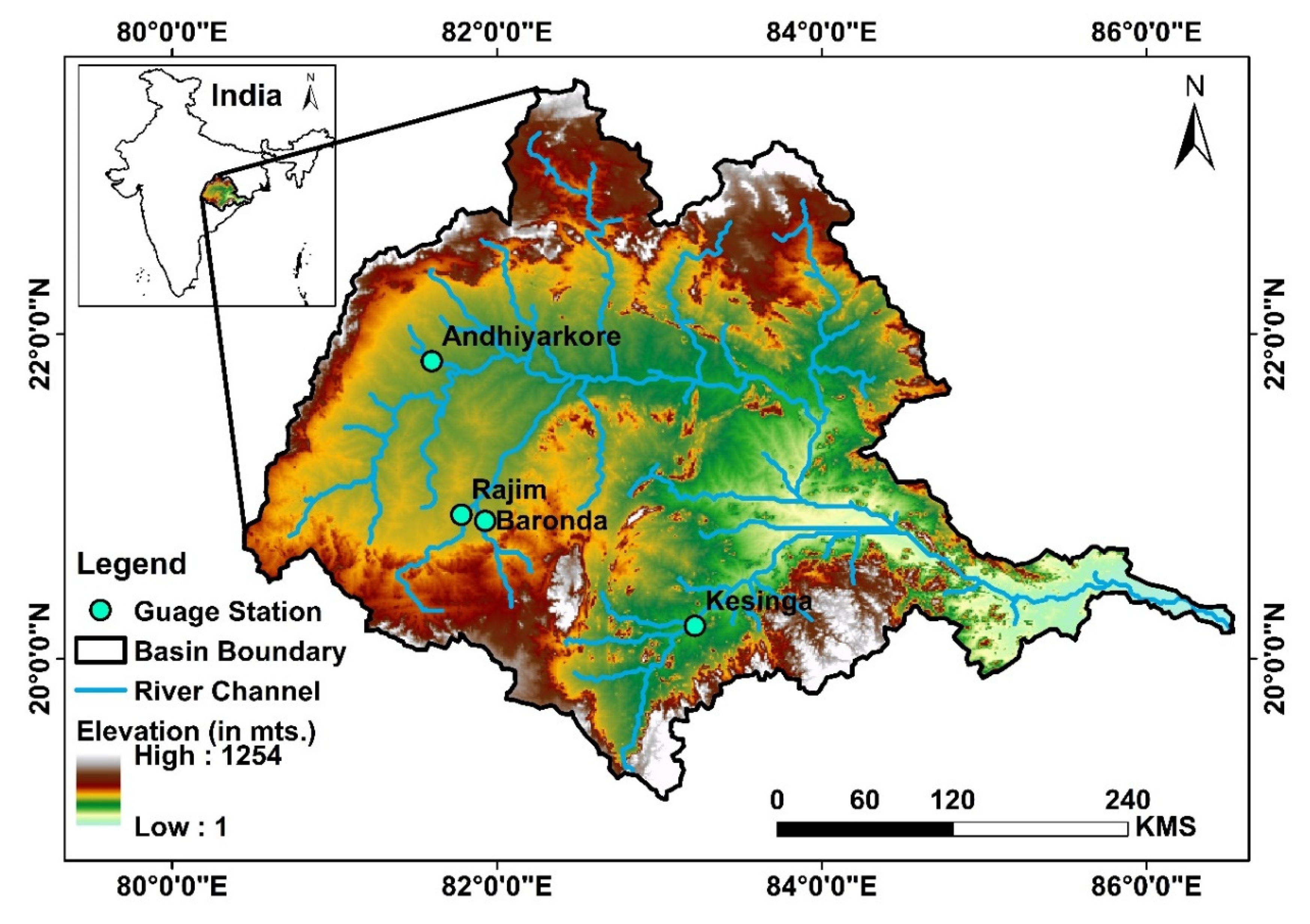
17]. Numerous studies have been conducted to determine how different factors impact streamflow generation. Water resources and river streamflow have been affected by climate variability and global warming. Hence, it is of great practical significance to study the response mechanism of hydrological process change for future water resource planning and management. The basin of Mahanadi is likely to experience severe flooding under the changing climate scenarios. The spatial and temporal variation of daily rainfall for 30 years over Mahanadi basin have been analyzed and the study concluded that the region experiences higher frequency and higher intensity of very heavy rainfall with less inter-annual variability [
29]. Average annual rainfall here is 1572 mm, of which 70% is precipitated during the south-west monsoon between June to October [
30]. The basin is highly vulnerable to floods and has been affected by catastrophic flood disasters almost annually. The Mahanadi was notorious for its devastating floods for much of recorded history, and consequently it is called the “sorrow of Odisha” [
30]. The problem of flooding still persists, and a lasting solution needs to be evolved. The Mahanadi belt is best known for its fertile soil and flourishing agriculture. The major portion of this river basin is agriculturally dominated (approximately 60%) followed by forest area (approximately 25%) mostly in the upper catchment [
31]. Though agriculture is dominant in the basin, the economic background of the farmers is quite low here in comparison to the rest of the country as agriculture is heavily dependent on rainfall and the irregular and erratic nature of has damaged many of them. As hydrology plays an important role in determining the growth of agricultural sector; therefore, studying the impact of climate variability on hydrology [
32,
33,
34,
35] is a major issue of concern. Hence, the pivotal role of climate in agriculture sector, the principal source of livelihood of the population and low economic background of the farmers in and around the basin, motivated the authors to investigate the impact of climate variability on streamflow [
36,
37,
38,
39] in terms of various climatic parameters in the basin region.
Streamflow of the Mahanadi river basin is mainly dependent on seasonal monsoon rainfall. About 85% of total rainfall occurs in the Mahanadi basin during monsoon season only. The analysis of the Mahanadi basin using the predicted data for the period, 2041–2060, revealed that in future due to climate variability, severe flooding will occur in delta region causing destruction in low-lying areas [
40,
41]. Among various sources of recurring climate variability, ENSO (El Nino Southern Oscillation), ENSO Modoki, Indian Monsoon, and IOD (Indian Ocean Dipole) are supposed to have great influence on water streamflow of the Mahanadi river basin. Hence, the main objective of this study is to investigate the relative and combined effects of Indian Monsoon and Indo-Pacific climatic modes on high streamflow events and flood frequency analysis in the Mahanadi river basin.
3. Data and Methods
Before analyzing the data, the homogeneity test was done using XLSTAT software. Though there are various tests for homogeneity, we used SNHT (Standard Normal Homogeneity Test) in our study. It is a widely used technique and applied to a series of ratios that compare the observations of a measuring station with the average of other remaining stations and so on. As far as the result is concerned the computed “p” value, i.e., 0.1, which is greater than the “alpha value”, i.e., 0.05; hence, the null hypothesis “H0” is accepted, which says the data are homogeneous [
44].
Climatology and anomalies of streamflow were calculated on daily basis from 1980 to 2013 for 34 years in total. The daily streamflow data for the four selected stations (Andhiyarkore, Baronda, Rajim, and Kesinga) were obtained from the “India-WRIS (Water Resources Information System)” site. High streamflow events were picked from the daily streamflow anomaly data based on a threshold of 1.5σ (σ stands for standard-deviation). Persistently high values for 6 days or more were combined to frame one extreme event. In addition to these, various climate indices were used to show the variability impact on daily streamflow like Monsoon Index (hereafter MI), El Nino Modoki Index (hereafter EMI), Oceanic Nino Index (hereafter ONI), Dipole Mode Index (hereafter DMI), and Nino3. Among various monsoon indices “Indian Summer Monsoon Index” is used, which is computed as follows:
is the means difference between U850 (U wind at 850 mb) over two regions with varied latitudinal and longitudinal extension as mentioned in Equation (1), where IM stands for Indian Monsoon.
EMI associated with El Nino Modoki (mEl Nino) and La Nina Modoki (mLa Nina) that influences the streamflow, was derived from Ashok et al. (2007). It is defined as mEL Nino (mLa Nina) with strong warming (cooling) in the central tropical pacific and cooling (warming) in the eastern and western tropical pacific [
45,
46]. This index is computed as:
Sea surface temperature (SST) means the water temperature close to the surface of the ocean. SSTA means sea surface temperature anomaly, which is a departure of prevailing temperature from average conditions.
The boxes in Equation (2) represents SST anomalies over region A (165° E–140° W,10° S–10° N), B (110° W–70° W, 15° S–5° N), and C (125° E–145° E, 10° S–20° N), respectively [
46].
ONI, believed to have strong impact on streamflow, is National Oceanic and Atmospheric Administrations (NOAA) primary index for monitoring the relative strength of El Nino Southern Oscillation (ENSO). It is related to strong anomalous warming/cooling condition in eastern tropical pacific and cooling/warming condition in western tropical pacific. It is calculated as taking the three-month running average ERSST.V4 (Extended Reconstruction SST. Version 4) SST anomalies in the Nino 3.4 (5° N–5° S,120° W–170° W) region.
DMI is used to represent the intensity of Indian Ocean Dipole by anomalous SST gradient between the western (50° E–70° E and 10° S–10° N) tropical Indian Ocean and the eastern (90° E–110° E and 10° S–0°) tropical Indian Ocean [
47]. A positive IOD (pIOD) phenomenon is described as the cooler than normal water in the tropical eastern Indian Ocean and warmer than normal water in the tropical western Indian Ocean whereas a negative IOD is identified as warmer than normal water in tropical eastern Indian Ocean and cooler than normal water in western Indian Ocean [
48].
Nino3 index is calculated by taking area average of SST anomalies in °C (degree Celsius) of region over eastern Pacific Ocean which is bounded by 90° W–150° W and 5° S–5° N.
To establish the relationship between streamflow and various climate parameters, correlation and partial correlation techniques were used. We used Pearson’s product moment correlation technique for the study. While correlation techniques establish a mutual association between two variables, partial correlation took place to find out the variable which had the most determining effect. Then partial correlation was conducted, being the relationship between two variables while controlling a third variable, because the third variable has shown a relationship to one or both of the primary variables.
Stepwise regression is a method of fitting regression models in which the choice of predictive variables is carried out by an automatic procedure. In each step, a variable is considered for addition to, or subtraction from, the set of explanatory variables based on some prespecified criterion. Among various approaches of stepwise regression analysis, backward elimination procedure was used in this calculation. This involved starting with all candidate variables, testing the deletion of each variable using a chosen model fit criterion, deleting the variable (if any) whose loss gives the most statistically insignificant deterioration of the model fit, and repeating this process until no further variables can be deleted without a statistically significant loss of fit. Though stepwise regression analysis was carried for all variables only the significant results were used in the study for analysis.
After analyzing the streamflow sensitivity to extreme flood events, we extended our analysis to the frequency distribution, Weibull’s plotting position method was used to compute the 34 years return period to identify the flood frequency within the Mahanadi river basin for policy makers and water managers. We assumed that the data followed a specific distribution (Gumbel or Extreme Value Type 1) (see
Section 4.5). We estimated the parameters of the distribution by using following cumulative distribution function (CDF):
where
is the observed maxima,
and
are location parameters, respectively, and computed as
(Here,
and
are the mean and standard deviation, respectively.)
4. Results and Discussion
4.1. Seasonality of Daily Streamflow
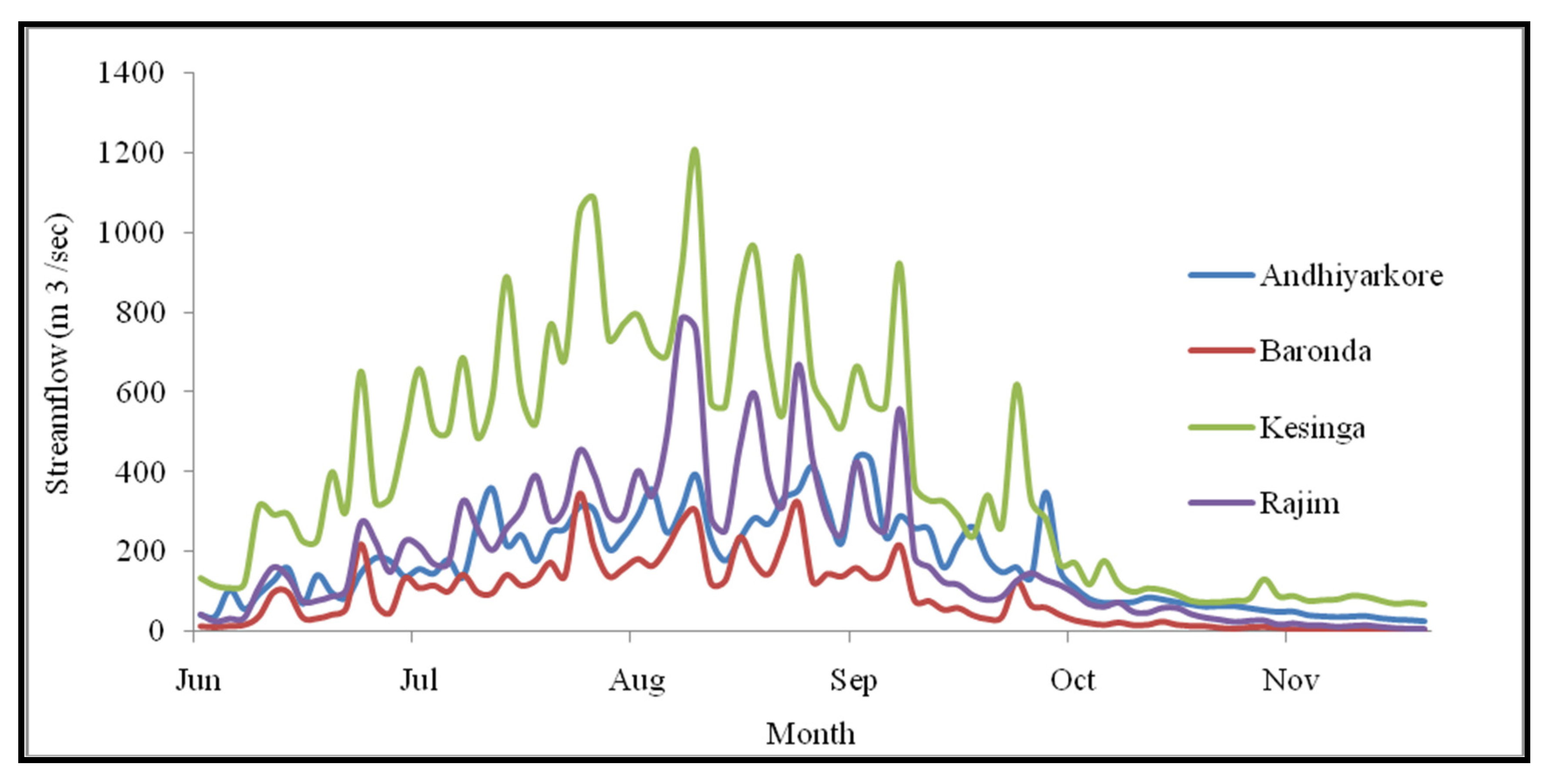
The daily climatology of the Mahanadi streamflows (
Figure 2) showed higher seasonal flows during the months of June–November and very less streamflow was experienced in the basin after October, i.e., from November to May (figure not shown) in all four stations. As already mentioned in the introduction, the Mahanadi is a monsoon led river, monsoonal rainfall feeds the streamflow of the basin. Monsoon starts in June and lasts till September in the Indian sub-continent. Hence, it is also clearly visible from the figure that high streamflow took place around mid-June and got lower by mid-September. The four stream gauge stations showed almost same pattern of seasonal climatology. To extract the high streamflow events, 1.5σ threshold was applied, and persistence of seven days or more was considered as one event. The peak streamflows were observed during monsoonal months which resulted into floods. Panda et al. [
49] in their study observed that the Mahanadi basin is characterized by a tropical monsoon (June to September) climate and more than 80% of the annual runoff occurs during the monsoon season. Moreover, these high streamflow events or floods [
50,
51] have a tremendous impact on the local population and ecosystem. Hence, to cope with this obvious impact of floods in the basin area, the study of climate variability impact on river water streamflow has become the need of the hour.
As shown in
Table 1,
Table 2,
Table 3 and
Table 4 the high streamflow events were calculated by taking into account the persistence flow for seven days or more, for all four stations separately during the JJA and SON seasons. The results display maximum dominance of Indian Monsoon on high streamflow events or flood events. Along with Indian Monsoon, La Nina, La Nina Modoki (mLa Nina), the positive Indian Ocean Dipole also has a significant role in influencing a high streamflow event.
4.2. Impact of Indian Monsoon
Monsoon plays a pivotal role in streamflow variability of the Mahanadi river basin. As it is a monsoon fed river, it faces heavy streamflow during the monsoon season, that is from June to September. Therefore, the correlation (values shown in
Table 5 and
Table 6) of streamflow anomalies with Monsoon Index were calculated for the JJA season and the SON season to quantify the impact of this climatic variability mode (Indian Monsoon). Pearson’s correlation coefficient calculation was followed to study the variability impact. An important thing to be mentioned here is that, while calculating correlation, the MI of the JJA season was taken into consideration with streamflow anomalies of the JJA season, but for the SON season, the MI of both the JAS and June, July, August and September (JJAS) seasons were taken into account for calculating Pearson’s correlation with streamflow anomalies of the SON season as the MI for the SON season was not available.
For calculating partial correlation, EMI was into consideration with MI, because it displayed high correlation with streamflow anomaly during these seasons. Hence, to measure the strength of Indian Monsoon, the effect of EMI was controlled. Based on the result, it was found that all station displayed a significant positive correlation with Indian Monsoon. The correlation values for Andhiyarkore, Baronda, Rajim, and Kesinga, during the JJA season, are 0.53, 0.38, 0.44, and 0.38, respectively. Similarly, with EMI, the streamflow also shows strong positive correlation, i.e., 0.37 for Andhiyarkore, 0.42 for Baronda, 0.51 for Rajim, and 0.36 for Kesinga. As far as partial correlation is concerned, only streamflow at Rajim and Kesinga stations showed negative correlation with MI, i.e., −0.2 and −0.72, respectively. This indicates the strong influence of EMI on the streamflow of these two stations. A similar thing was found with Baronda station when partial correlation of streamflow with EMI was calculated, the result was found to be −0.28. It undermines the impact of EMI on the streamflow at Baronda station.
The impact of Indian Monsoon was proved from correlation and partial correlation values displayed in
Table 5 and
Table 6. Apart from climate factors, land use and land cover need to be studied for the quality of water, as argued by Jun, and Wang and Hejazi [
13,
52], for better management of water resources in a basin.
4.3. Impact of Indo-Pacific Climate Variability Modes
Other than Indian Monsoon, the study also attempts to understand the regional manifestation of Indo-Pacific climate impacts, because it is well known that the Indo-Pacific climate largely influences large-scale phenomenon such as monsoons. It can be said that the strength of Indian Monsoon, whether strong or weak, largely depends on the nature of Indo-Pacific climate variability parameters. Therefore, the relationship between river streamflow and climate variation are very important since the latter has a direct influence on Monsoon as well as on rainfall variability.
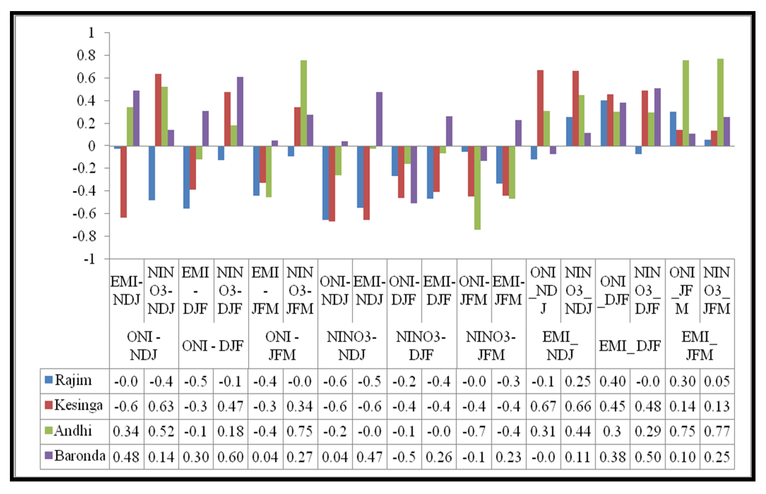
To quantify and show the extent of impact of Indo-Pacific variability modes, partial correlation was calculated between streamflow anomalies during the JJA season and ONI, EMI, and Nino3 of the NDJ (November–January), DJF (December–February), and JFM (January–March) seasons, respectively (
Figure 3), and DMI of the SON (September–November) and OND (October–December) seasons, respectively (
Table 7).
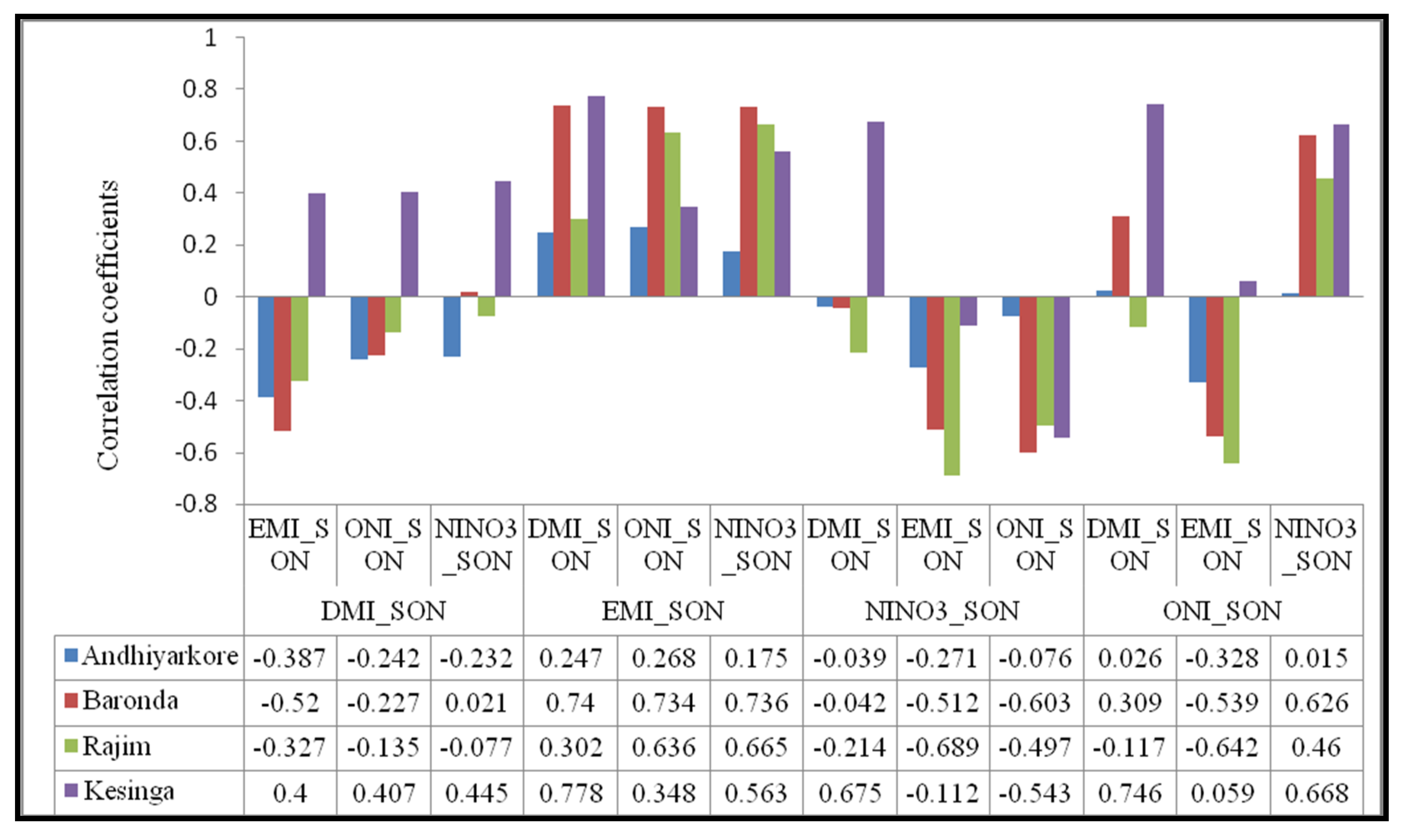
Similarly, partial correlation values between streamflow anomalies of the SON season and climate variability indices, i.e., ONI, EMI, Nino3, and DMI of the SON season are displayed (see
Figure 4). It is noteworthy to mention here that the partial correlation was calculated between event specific years and climate variability indices of previous years for the JJA season because climatic phenomena in the Pacific Ocean are in their peak occurrence during this time period, i.e., November–March. Hence, to show the impact of an El Nino or La Nina event on streamflow in Mahanadi Basin, partial correlation was calculated. Likewise, Indian Ocean Dipole has its occurrence in the Indian Ocean during the SON and OND seasons. Hence, to see the effect of IOD on high streamflow event in the basin, DMI of SON and OND was taken into consideration. However, while calculating partial correlation between streamflow anomaly of the SON season and climate variability modes, the index values of same year were taken.
The link between streamflow of JJA and SON seasons and global climatic variability modes (ONI, Nino3, EMI, and DMI) is shown through
Figure 3 and
Figure 4 and
Table 7. The results show the impact of global climate variability modes on the streamflow of Mahanadi Basin. Because of the proximity to coast of the Bay of Bengal, the Mahanadi river basin is sensitive to the large-scale coupled atmospheric-oceanic circulation modes such as the El Nino Southern Oscillation (ENSO) and Indian Ocean Dipole (IOD) [
53]. In the study of Maity et al. [
54], it was observed that both large scale global atmospheric inputs owing to hydroclimatic teleconnection and local inputs feature as important inputs in streamflow prediction of this basin. Hence, from our results, it was also confirmed that Indian monsoon affects streamflow the most, and that the basin experiences a moderate impact of global climatic variables.
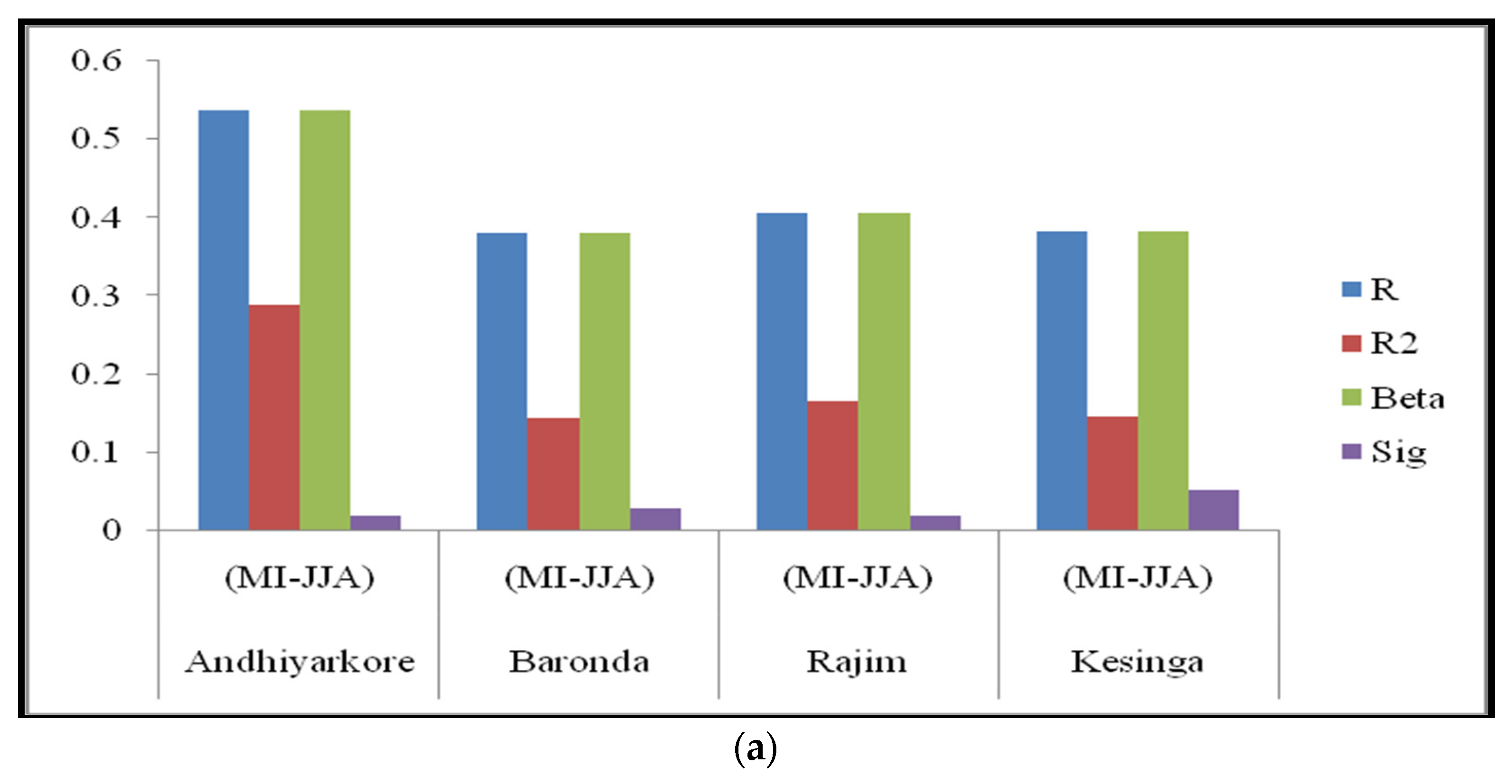
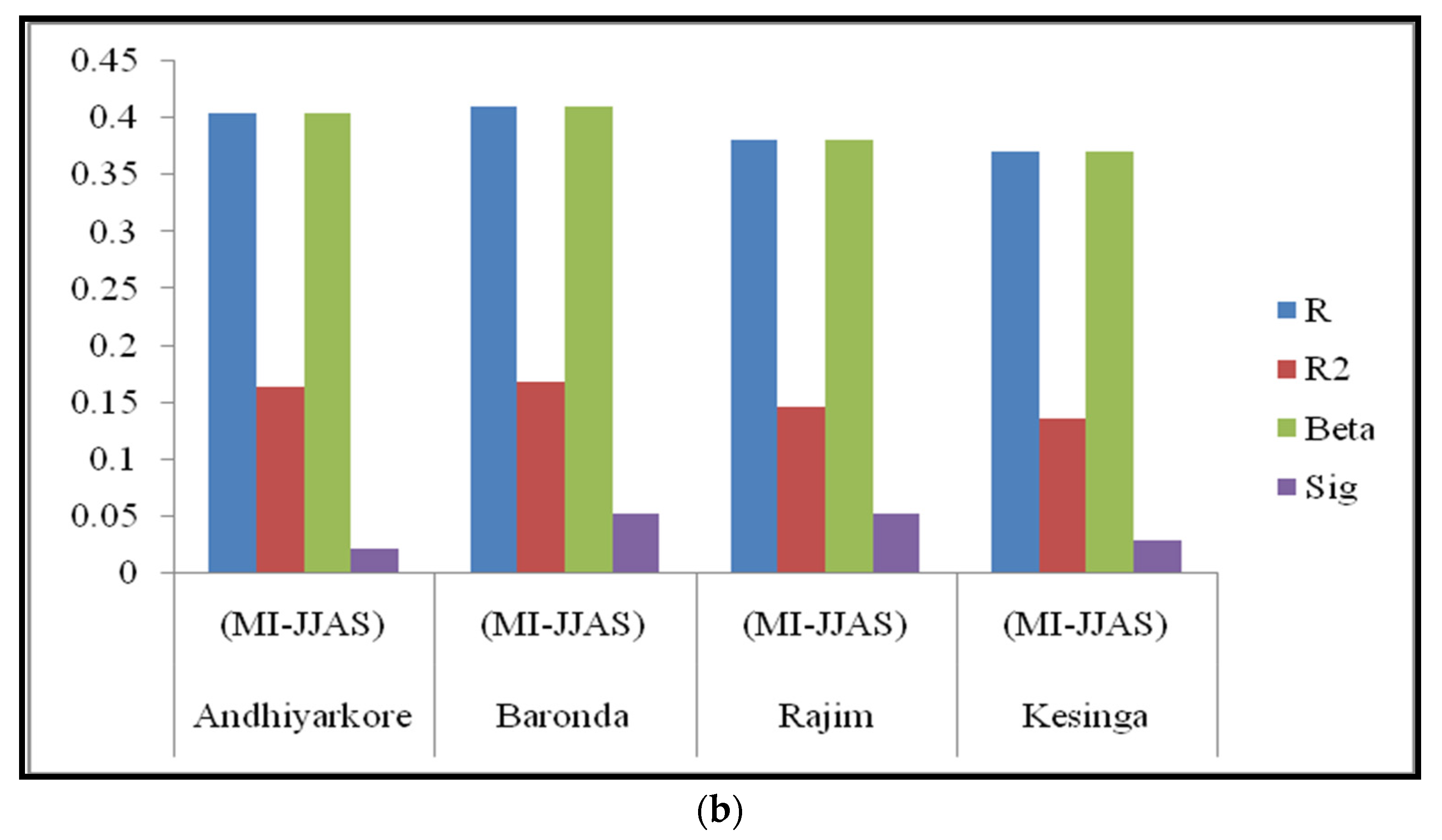
4.4. Stepwise Regression Analysis for Four Stations
Stepwise regression is a method of fitting regression models [
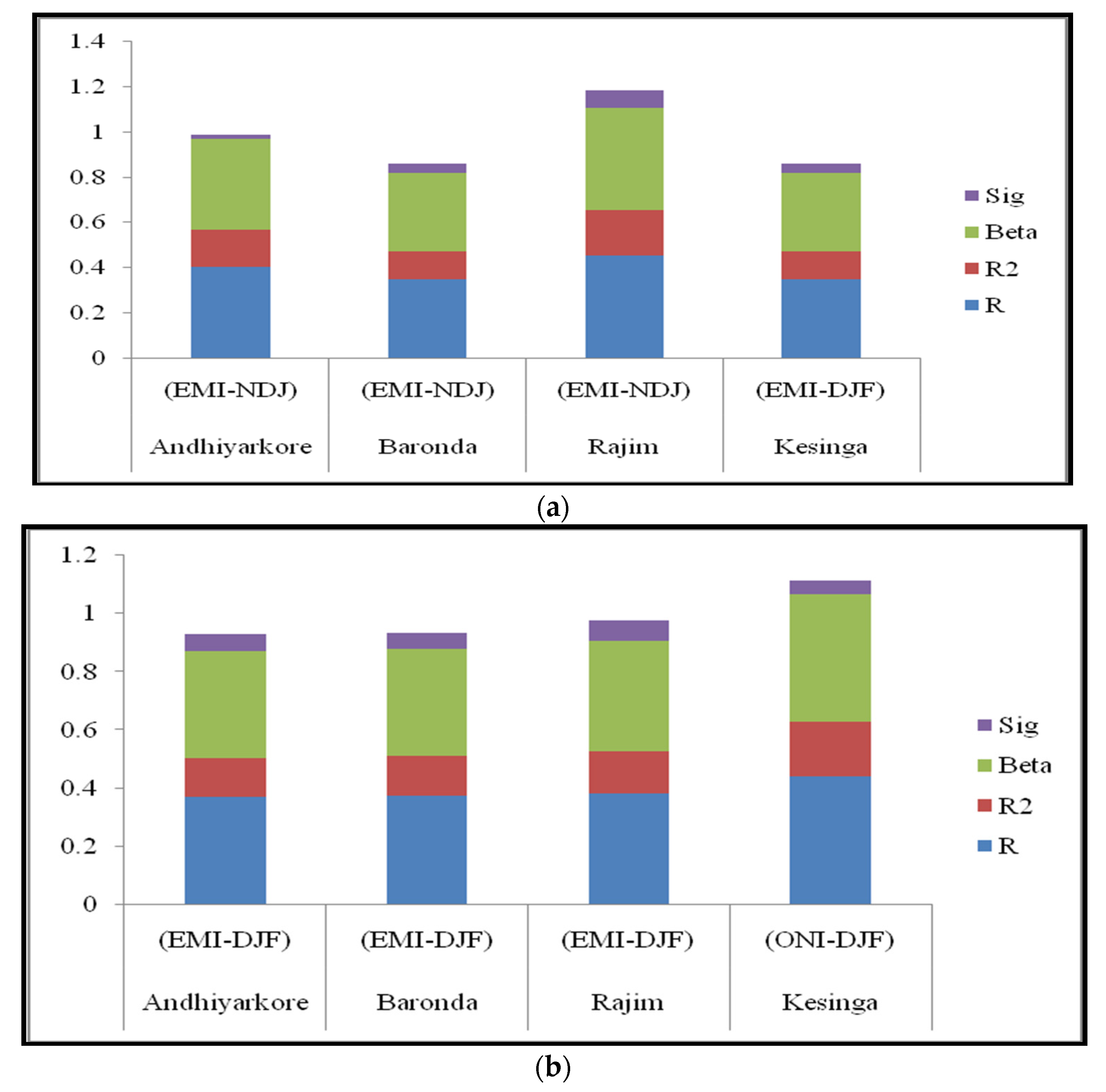
55] in which the choice of predictive variables is carried out by an automatic procedure. In each step, a variable is considered for addition to, or subtraction from, the set of explanatory variables based on some pre-specified criterion. This method evaluates the independent variable at each step, adding or deleting them from model. Hence, in this study, stepwise regression analysis with backward elimination method was incorporated to choose the best predictor for streamflow of four different stations in both the seasons, i.e., JJA and SON (
Figure 5a,b and
Figure 6a,b). Four values have been presented in both the figures those are R, R
2, Beta, and Sig. “R” value refers to the correlation value, where R
2 implies to the coefficient of determination, Beta is the correlation coefficient range from 0–1, finally, the significance value suggests the strength of the test. It was found that MI-JJA proved to be the best predictor among MI-JJA, MI-JJAS, and MI-JAS, for streamflow of the JJA season in four stations. However, for the SON season, MI-JJAS played the role of best predictor in four studied stations. Likewise, when EMI, ONI, and Nino3, of NDJ and DJF were taken as independent variables to predict JJA streamflow of four stations, then it was found that EMI-NDJ was the best predictor for Andhiyarkore, Baronda, and Rajim stations, and that EMI-DJF was the best predictor for Kesinga season. For the SON season EMI-DJF played a dominant role for streamflow prediction of Andhiyarkore, Baronda, and Rajim stations, but ONI-DJF proved to be the dominant factor in predicting Kesinga station.
4.5. Flood Frequency Analysis
We extended our analysis to the frequency distribution and return period of the streamflow with annual JJA and SON maximum streamflow values from the observation datasets for the period 1980–2013 (34 years). Many recent studies have highlighted that the flood events mostly exhibit a better fit with a specific distribution of Gumbel or Extreme Value Type 1. We assumed that the data followed a specific distribution (Gumbel or Extreme Value Type 1) [
56,
57,
58].
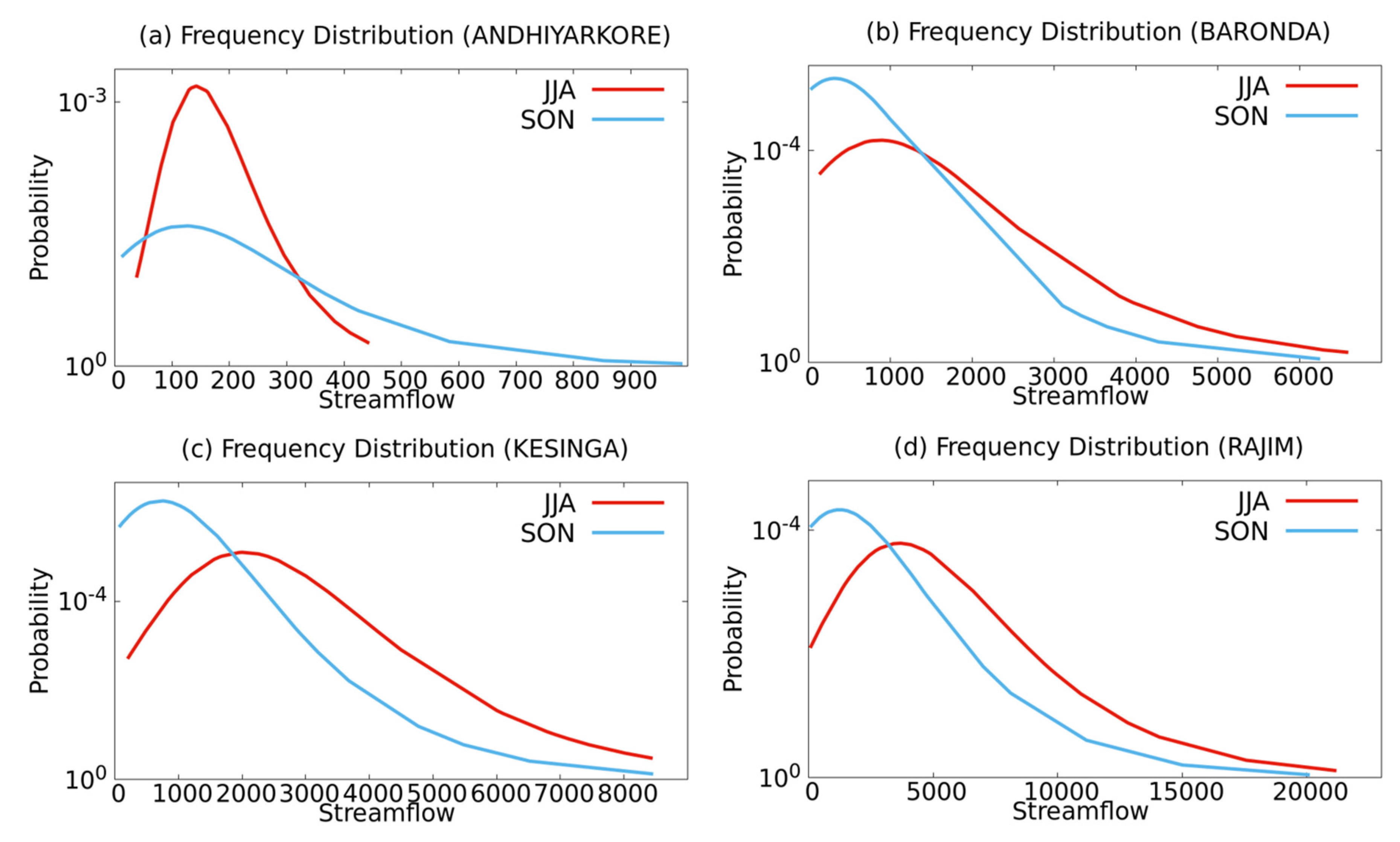
Figure 7 shows the frequency distribution of annual JJA and SON daily maximum streamflow with respect to Gumbel distribution over four river areas, viz., Andhiyarkore (
Figure 7a), Bronda (
Figure 7b), Kesinga (
Figure 7c), and Rajim (
Figure 7d). We found that the probabilities of streamflow values exceeding ~2000 m
3 s
−1 were higher in JJA at the Bronda, Kesinga, and Rajim river areas, while that of lower to ~2000 m
3 s
−1 were higher in SON (
Figure 7b–d). The streamflow values at the Andhiyarkore river area were likely to have less runoff (~450 m
3 s
−1 maximum in JJA and ~1000 m
3 s
−1 in SON), very small catchment, and located at higher elevation, as shown in
Figure 1 (
Figure 7a). However, the occurrence of streamflow in the range between about 50–320 m
3 s
−1 was higher in JJA compared to that of in SON.
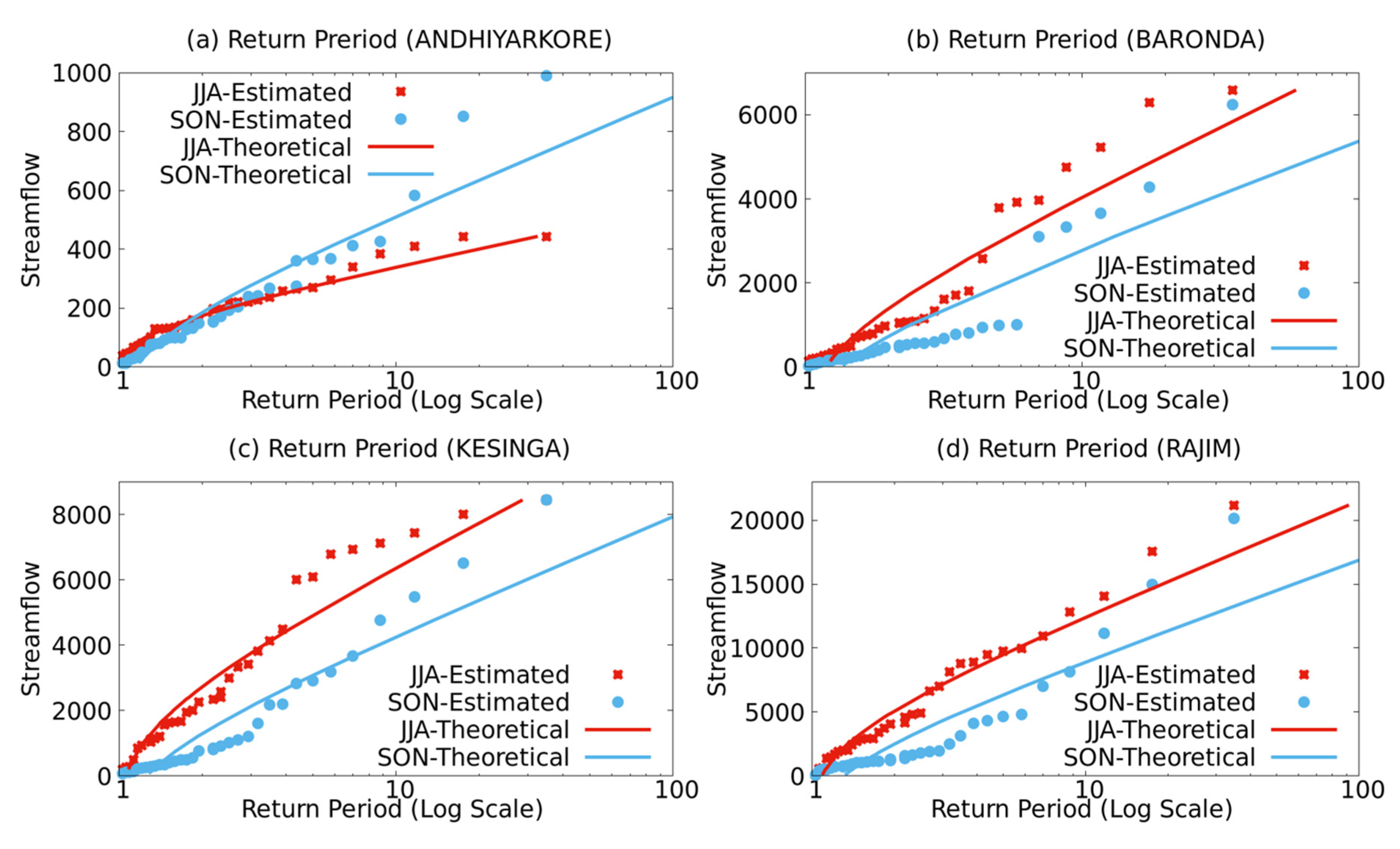
Weibull’s plotting position method along with Gumbel distribution was used to compute the return period and the results are shown in
Figure 8. The return period obtained from Weibull’s plotting position is referred as “estimated” and that from Gumbel distribution is referred as “theoretical”. Results indicate that the return periods of streamflow values below ~400 m
3 s
−1 are within 10 years at Andhiyarkore river areas in both JJA and SON, while that of higher values are within 34 years, although their occurrence are less (
Figure 8a). The return period of streamflow at the Baronda, Kesinga, and Rajim river areas are noticed to be faster in JJA compare to that of in SON (
Figure 8b–d). The 10 years return period of streamflow at the Baronda river area in SON corresponds to the value ~3500 m
3 s
−1, while that of in JJA corresponds to the value ~5000 m
3 s
−1 (
Figure 8b). Similar characteristics with higher streamflow values are noticed at the Kesinga and Rajim river areas.
Overall, the return periods of streamflow in JJA shows robust results in both the estimations (Weibull and Gumbell), while in SON they show deviations after 10 years. The higher streamflow was found to have occurred more frequently in JJA at Bronda, Kesinga, and Rajim stations and their return periods are expected to be faster in JJA, indicating more floods in JJA over the Mahanadi river basin during monsoon season. The reason could be associated with the summer time warming over India which would increase the moisture holding capacity in the atmosphere according to the Clausius–Clapeyron relationship (7% per degree rise in temperature) and may lead to more rainfall over the region [
59,
60,
61]
5. Conclusions
Anomalous coupled ocean–atmosphere phenomena generated in the tropical oceans produce global atmospheric and oceanic circulation changes that influence regional climate conditions even in remote regions and eventually regional hydrology. In this study, the daily river streamflow characteristics with the climate variability, e.g., IOD, ENSO, ENSO Modoki, Indian Monsoon, and NINO3 were analyzed. Here, peak streamflow seasons (June–November) were taken into consideration for four gauge stations (Andhiyarkore, Baronda, Rajim, and Kesinga) of the Mahanadi river basin. The results show the stronger influences of Indian Monsoon on the extreme high streamflow events during the JJA and SON seasons. The impact of ENSO and ENSO Modoki on river extremities were also found to be significant during these two continuous seasons. Additionally, prevalence of positive IOD during event years were noticed. Since most of the climate variations in the Indo-Pacific sector are predictable on seasonal to inter-annual scales, the regional impacts of those, like direct influence on Indian monsoon and vis-a-vis on streamflow can be made beforehand. Moreover, these predictions can be extended to help the local communities dependent on streamflow. It has been found that among various indices of MI, MI-JJA has a determining effect for the streamflow of the JJA season and MI-JJAS has the dominant role in determining SON streamflow. Likewise, when stepwise regression model was calculated using the EMI, ONI, and Nino3 indices, then EMI of both NDJ and DJF play vital roles among all pacific climate variability modes in affecting streamflow of Mahanadi during the JJA and SON seasons. Furthermore, flood frequency analysis at Baronda, Kesinga, and Rajim were higher in JJA compared to SON. Return period indicates more floods in JJA over the Mahanadi river basin.
In addition to the societal impact, this study can be used to attract the attention of the climate and hydrology research groups to investigate those climatic links further. This study clearly displays the direct impact of Indian Monsoon and other Indo-Pacific climatic variability phenomena (ENSO, ENSO Modoki, Indian Ocean Dipole, and Nino3) on river water streamflow. This scientific contribution shows a dominant influence of climate variability as compared to any other factors responsible for streamflows on longer time scales.

 ,
, 


