Localization of Groundwater Contaminant Sources Using Artificially Enhanced Catchment

Abstract

The localization of groundwater contaminant sources is the first and most fundamental step when dealing with site contamination problems. This paper presents a novel approach for groundwater pollution source identification in a site with low-velocity groundwater in which a strategy of an artificially enhanced catchment is adopted. The distance from a pumping well (artificial sink) to the source zone (unknown source) is calculated by integrating the concentration time series and well flow. Then, the orientation of the source well is delineated by applying the method of distance intersection. This method is suitable for an approximately homogeneous aquifer with average hydraulic conductivity ranging from 1 × 10⁻⁶ to 1 × 10⁻⁵ m/s and a contaminant whose transport process can be generalized to convective migration. The developed method was applied to an industrial contaminated site using three pumping wells and two observation wells. The results demonstrated that four potential source positions were identified. Among these, two positions situated near the production workshop were excluded by observation well responses. The remaining two positions located near the drain were identified as preferred treatment sources. Electrical prospecting showed source orientation consistent with the artificially enhanced catchment results. This proved that the method is effective and provides an alternative tool to help solve the problem of source identification in the first stage of remediation in sites with low-velocity groundwater.

1. Introduction

Groundwater contaminated sites constitute serious threats to water quality. The pollution source is a key element of conceptual site models. Locating and removing contamination sources is an essential step in site risk management. Pollution source identification involves determining the source location, source magnitude, and release history [1]. Accuracy of source localization will influence the efficiency and cost of remediation.

Three events occur after a contaminant is released into groundwater. These are advection, dispersion, and reaction [2]. A contaminant disperses as a plume in the subsurface environment via these functions. Contaminants in groundwater are often detected at an arbitrary point of the plume. A monitoring network can then be designed and optimized for characterizing the plume by interpolating results from point-scale sampling [3,4,5]. By combining plume information with contaminant migration rules, the source can be located as an inverse problem. However, this inverse problem has the limitations of instability and non-uniqueness that are caused by irreversibility of the contaminant transport process in a saturated porous medium. One type of method for solving the inverse problem is to calculate backward in time. Bagtzoglou and Atmadja [6] reviewed three mathematical methods for backward source identification. These included probabilistic and geostatistical simulation approaches [7,8], analytical solution and regression approaches [9], and direct approaches [10]. Another approach for solving the source identification problem is to use optimization techniques [11]. By linking the groundwater flow and transport model with optimization techniques, the source identification problem can be solved forward in time [12,13,14]. The objective of optimization methods is to minimize the difference between observed and computed measurements.

For both backward-in-time and forward-in-time identification methods, the quality and quantity of observational data is critical for successfully achieving source localization. When the media is heterogeneous, identification of the contamination source relying on inadequate samples yields imprecise results [15]. This is especially true in porous media with low permeability (hydraulic conductivity from 1 × 10⁻⁶ to 1 × 10⁻⁵ m/s), such as silt or silty sand. In these types of porous media, non-reactive pollutants are transported by low-velocity advection and dispersion. When contaminants are distributed close to the source zone instead of spreading as a plume strip, a monitoring network only depending on conventional network density may overlook information from an unknown source zone. Few wells are available in a site investigation phase and it is consuming to drill new monitoring wells without additional source information. In China, the main industrial development zones are located in the south-east coastal areas. The sediments in these regions are relatively low-permeability. Groundwater contaminant source localization at such sites is challenging during the investigation and remediation phases. In addition, the pollution release history is complex and multiple pollution sources may be involved in a single site. This makes it more difficult to identify pollution sources. An effective method for locating the source(s) of groundwater pollution and for remediation design is needed in these areas.

Information relating to aquifers can be obtained at a larger scale by pumping. This strategy is used in the integral pumping test (IPT) method [16,17]. Pumping is implemented along a control plane (CP) located perpendicular to the direction of groundwater, downstream of the potential pollution source. Samples are taken from the pumped water at regular intervals. Contamination distribution along a CP can be converted to a concentration time series using analytical approaches [18] or numerical methods [19]. The IPT method can calculate mass flux along one CP [20], estimate natural attenuation rate between two CPs [21], and backtrack source information upstream from the CP [22,23]. The IPT method can be used for contamination characterization in combination with other methods [24,25]. Compared with point-scale sampling [26,27], the IPT method can obtain more information about the contaminated aquifer by increasing the sampling volume and reducing small scale variability. However, the uncertainty of the IPT method derives from a strong concentration gradient [28] and plume position relative to the pumping well [29]. Leschik et al. [30] studied the optimal sampling schedules for IPT. Based on inversion assumptions and positions of the wells, the IPT method is suitable for studying plumes when the aquifer has high hydraulic conductivity. Thus, using the IPT method to calculate concentration distribution along a CP is effective under strong hydrodynamic conditions. However, the source zone location requires further evaluation. In low-permeability aquifers, it is difficult to trace the source of pollution backwards for a low hydraulic gradient.

As a result, local high-concentration pollution sources might be ignored for inadequate point-scale sampling. It is not feasible to backtrack the source zone using the concentration distribution obtained from an IPT. In view of the weak hydrodynamic conditions and irregular contamination distribution in low velocity flow fields, here we develop a source identification method based on an artificially enhanced catchment. The artificial source–sink relationship between a pumping well (artificial sink) and a source zone (unknown source) is established to identify the position of the source. Concentration time series and well flow theory are used to calculate the distance from the unknown source to the pumping well. The potential source is subsequently located by intersecting the catchment areas obtained from multiple pumping wells. This article shows the theory, steps, limitations, and field test results of the new method.

2. Model and Methodology

2.1. Theory of Method

According to Darcy’s law (Equation (1)), the velocity of groundwater flow is determined by the hydraulic conductivity (K) of an aquifer and the hydraulic gradient (dh/dl). The groundwater flow velocity is slow for low values of K and dh/dl in shallow aquifers of a coastal plain.

$$v=-K\left(\frac{dh}{dl}\right)$$

(1)

where v (L·T⁻¹) is the velocity, K (L·T⁻¹) is the hydraulic conductivity, and (dh/dl) (-) is the hydraulic gradient.

In a low-velocity groundwater flow field, conservative solutes migrate through weak convection and dispersion. Therefore, a point-scale and high-concentration groundwater pollution “source zone” is formed. The source zone in such a condition is easily ignored using the point-scale sampling approach. (Figure 1a).

Pumping can accelerate groundwater flow and enhance convective migration of solute. By monitoring and interpreting the solute concentration versus time series (C-t series) in the pumping well, the solute concentration distribution information in a wider area around the pumping well can be obtained. This strategy has been applied in the IPT method; however, only the absolute value of the C-t series is employed for concentration interpretation. Bockelmann [21] discussed four scenarios of the relationship between C-t series features and pumping well position in the IPT method. The trend and inflection point of the C-t series are different in each scenario. The process of identifying the solute concentration variation characteristics indicates the recharging process from outside to the pumping well.

This method is suitable for determining the location of a point source. A local high-concentration pollution zone is formed around the point source. The concentration of the point source pollutant is always higher than that of the high-concentration pollution zone. The method assumes that the source term does not change with the effect of pumping. The concentration of pollutants in the pumping well is much lower than that in the high-concentration source area. Under the effect of artificially enhanced hydraulic gradient, the contaminants in the high-concentration pollution zone will migrate to pumping wells. Due to the relatively small amount of water being pumped from a low-permeability aquifer, the pumping only affects the high-concentration pollution area, and the concentration of the point source remains invariable. The location identified by this method is the boundary of the high-concentration pollution area.

2.2. Model Development

2.2.1. Source–Well Response Establishment

In this model, wells with a high concentration of point-scale sampling are chosen as pumping wells in order to move closer to the potential source zone. When pumping is implemented near the source zone, an artificial source and sink relationship between source zone and pumping well (source and well) is established. The measured C-t series variation represents the recharging process from source to well.

In homogeneous, isotropic, and low-permeability aquifers, the hydraulic gradient formed by a pumping well is higher than in the natural state, so the natural groundwater flow can be ignored during the pumping process. In such conditions, the flow field formed by pumping is a radial symmetrical flow field [31]. The solute transport can be treated as a horizontal convection process. The transport velocity of solute to the pumping well (v_r) can be calculated according to Equation (2) [32].

$$v_r=-\frac{q_0}{2\pi h_0{n}_e}\frac{1}{r}$$

(2)

where v_r (L·T⁻¹) is the radial flow velocity, q₀ (L³·T⁻¹) is the pumping rate, r (L) is the radial distance to the pumping well, h₀ (L) is the aquifer thickness, and n_e (-) is the effective porosity.

2.2.2. Source–Well Distance Calculation

When solute from the source zone has transported to a pumping well, solute concentration in pumped water will present a sigmoid increased course. In this model, the period from the beginning of pumping to the time when solute concentration has increased to 50% of the total increment is defined as the transport duration. This time is recorded as t_a. A representative S-type curve Boltzmann function (Equation (3)) is chosen for C-t series fitting to calculate the time t_a.

$$C=\frac{C_1-C_2}{1+\exp \left(\frac{t-t_a}{dt}\right)}+C_2$$

(3)

where C₁, C₂ (M·L⁻³) are the initial and final concentrations before and after contaminant transportation to the well, t_a (T) is the center of the curve, and dt (T) is the time constant.

Utilizing the C-t series fitting and groundwater well flow calculation, the solute transport time (t_a) and velocity (v_r) are obtained. The source–well distance (l) can be calculated according to Equations (4)–(6).

$$dr=v_{r}dt$$

(4)

$${{\displaystyle \int }}_0^{l}rdr={{\displaystyle \int }}_0^{t_a}\frac{q_0}{2\pi h_0{n}_e}dt$$

(5)

$$l=\sqrt{\frac{q_0}{\pi h_0{n}_e}{t}_a}$$

(6)

where l (L) is transport distance from potential source to the pumping well (radius of the catchment area), q₀ (L³·T⁻¹) is the pumping rate, h₀ (L) is the aquifer thickness, n_e (-) is the effective porosity, and t_a (T) is the contaminant transport duration, which can be obtained through C-t series fitting.

For non-conservative solutes, the retardation factor can be used to correct the migration distance. Equation (7) can be used to calculate the distance considering retardation factor.

$$l_R=\frac{l}{R}$$

(7)

where l_R (L) is transport distance from potential source to the pumping well considering retardation factor, l (L) is the transport distance from the potential source to the pumping well for conservative solute, R (-) is retardation factor.

In real sites, constrained by the low-permeability medium, parameters should be designed before pumping. The appropriate well location will help shorten the identifying time and decrease secondary pollutant spread by pumping. The distance between pumping wells should be satisfied to overlay the catchment area of adjacent pumping wells. In addition, suitable pumping rates and duration need to be determined to keep the pump lasing and to control the costs of the pumping operation and extracted water treatment.

2.2.3. Source–Well Orientation Identification

Because the flow direction is radial during pumping, the potential source may be located at any position of a circle with its center at the location of the pumping well and a radius of l. This circle is defined as the catchment area of a potential contaminant source (dashed circle in Figure 1b). The distance intersection method is used to acquire the source orientation by combining multiple pumping wells. For the example of two pumping wells, in which the wells’ positions are known, the source–well distance can be calculated from each well, and the intersection points will be determined according to the relationship of the two circles.

The catchment area radius of two pumping wells are defined as l₁ and l₂ (l₁ > l₂), and the distance between two wells as s. If s > l₁ + l₂, the potential source zones of two wells are not the same, that is, more than one potential source zone exists. If l₁ – l₂ < s < l₁ + l₂, the potential source zone is located within the intersection points. There are two intersection points when the two circles intersect (Figure 1c).

Observation wells outside the catchment area can be used for selection of intersection points. An observation well represents one of the recharge directions of the pumping well. When the concentration of the observation well does not increase during pumping, it indicates that the high concentration of solute is not moving from the direction of this observation well. Defining one observation well as representing one quarter of a capture zone, a line can be drawn from the observation well to the pumping well. A right angle, using this line as an angle bisector, will overlap with the catchment area and form a sector zone (blue straight lines in Figure 1c). The intersection point in this zone will be excluded from the potential contaminant sources. In this method, the two intersections of two circles are the locations where the pollution source may exist. The pollutant concentration of groundwater in observation wells near the intersection can be further analyzed to identify the location of the pollution source. We divide the area around the pumping well equally according to the number and location of observation wells around the pumping well. When there are few observation wells in the study area, we preliminarily set the pumping well as the center and divide the study area into four 90° sectors. Then we determine the approximate location of the pollution source by comparing the concentration of pollutants in monitoring wells of different sectors. If the observation wells around the pumping well are densely distributed, the angle can be set according to the distribution position of the monitoring wells. And the study area is divided into more small sectors to help determine the location of the pollution source more accurately.

Combining the distance and orientation between the source and well, the potential source position can be identified in sites with low-velocity groundwater. The identified source position is the boundary of a high-concentration pollution area. The main direction for subsequent phases of investigation and remediation can be found through the application of the new approach. The magnitude and shape of the total source zone distribution are not determined in this method.

3. Field Test

3.1. Field Test Site Description and Point Scale Sampling

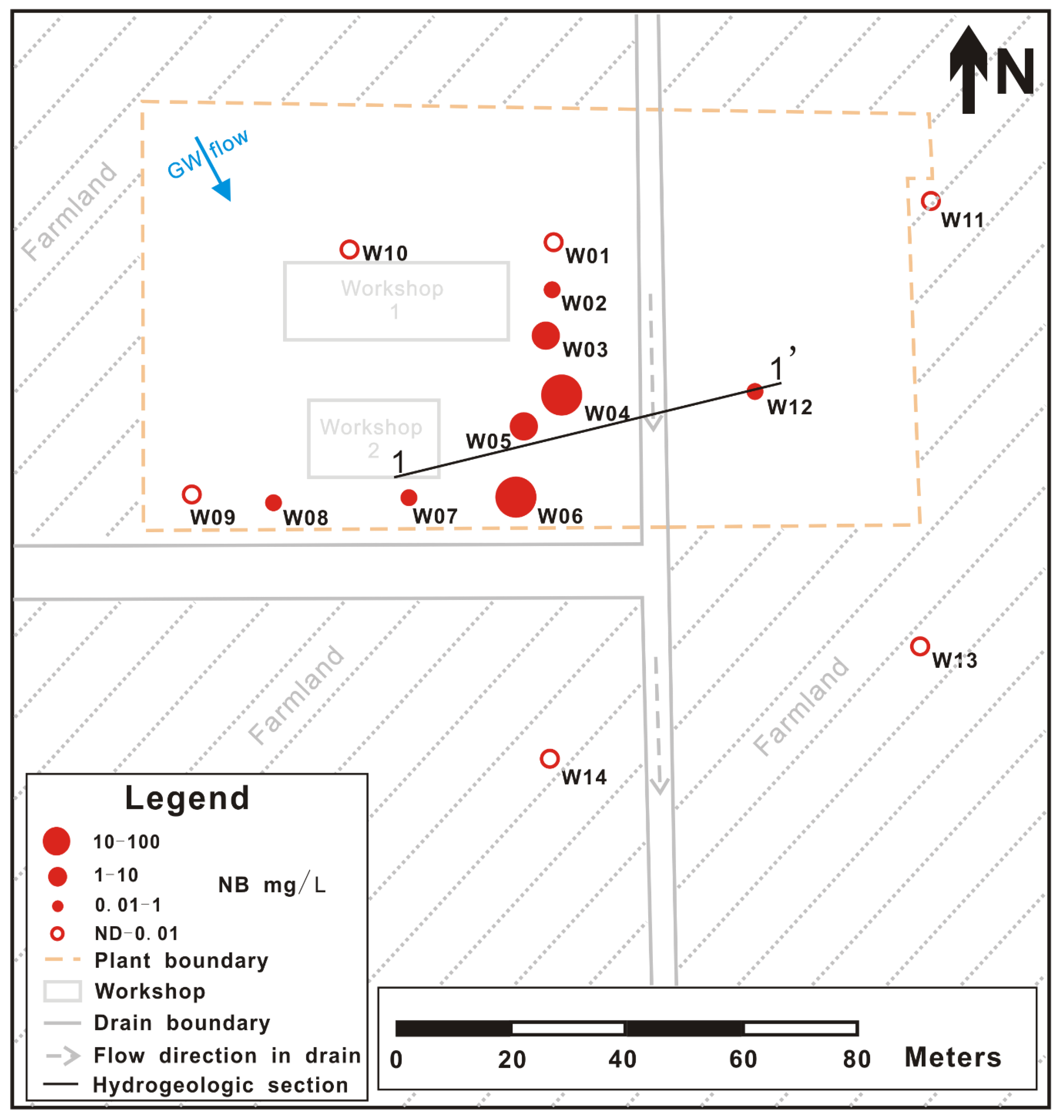
The study site was located in the city of Cangzhou on the eastern part of the North China Plain. The total area of the site is about 12,000 m². The area has flat morphology with elevation of 7.50 m. A dye intermediate production plant operated at this site from 1988 to 2011. Nitrobenzene (NB) was one of the main chemicals used in production. According to plant records, production workshop 1 and 2 were production areas of the plant. A north–south drain with anti-seepage measures was situated about 1.5 m below ground level. Wastewater was discharged by the plant to the drain and flowed to the south from 1988 to 1996. Although there were anti-seepage facilities at the bottom of the drain, there was a possibility of local rupture, and the specific release location was not clear. The ground rupture of workshop 1, workshop 2 and the drain were the potential source locations.

The geology and hydrogeology of the site were investigated in detail. Drilling results within the scope of the site indicated that the stratum was composed of Quaternary silt and silty clay. Groundwater was buried in a weak confined aquifer system with a depth of about 5.7 m. Silt was the main aqueous medium. The silty clay lens exists locally. The bottom layer of the aquifer was a continuous silty clay layer with a depth of about 2 m. All the monitoring wells in the site were fully penetrating wells. Water level monitoring indicated that groundwater flowed from north to south with a hydraulic gradient of 3 × 10⁻³ under natural flow conditions. Pumping tests in well W05, W07, and W09 demonstrated hydraulic conductivity of the aquifer system was 9.37 × 10⁻⁶, 1.43 × 10⁻⁵, and 6.19 × 10⁻⁶ m/s, respectively. The standard deviation of the hydraulic conductivity was 4.09 × 10⁻⁶ m/s. The aquifer system was treated as approximate homogeneous based on aquifer structure and parameters. The aquifer structure and pumping tests’ results are shown in Supplementary Materials. The effective porosity of the aquifer was 0.15. The hydraulic gradient and hydraulic conductivity make this site an example of low-velocity groundwater. A hydrogeological section is shown in Figure 2.

Groundwater samples were taken at the site using existing monitoring wells. QED low-flow sampling with Micro-Purge equipment was used for groundwater sampling in the wells. Eight of 14 wells had detectable levels of NB. Point-scale sampling results indicated a large concentration gradient ranging from 0.001 to 62.3 mg/L within a relatively short distance of about 15 m. The high concentrations of NB were found emerged in wells W03, W04, W05, and W06. These four wells were located in the eastern part of workshops 1 and 2. The concentration of NB in the remaining wells was less than 1.00 mg/L. A site map with NB concentrations is shown in Figure 3.

In groundwater environment of the site, the migration process of NB includes convection, dispersion, adsorption, and biodegradation. NB in wastewater can be degraded, assisted by microorganism [33,34]. NB in groundwater biodegradation in different conditions was well fitted by the Monod equation and the q_max values varied from 0.018 to 0.046 h⁻¹ [35]. Monitoring results indicated that NB concentration degraded 8.9% within two years measured in well W04. So within the field test duration (95 days), the effect of biodegradation on the concentration of nitrobenzene is not considered in this study. In addition to NB, a high concentration of sodium and chloride ions was detected in groundwater. NB and inorganic ions were released to the groundwater simultaneously according to site history. Taking sodium ion as an example, the monitoring results indicated that the high concentration areas of sodium ions and NB are located at the same position. There were differences in the migration characteristics between sodium ion and NB. It was possible to evaluate the retardation factor R = L_Na/L_NB, where L_Na (L) is plume length of sodium ion, and L_NB (L) is plume length of NB. The sodium ion concentration of natural groundwater in the study area was relatively high. The sodium ion concentration in the groundwater upstream of the site was 1720 mg/L. The W03 well had the highest sodium ion concentration in the site, which was 8180 mg/L. The W03 was used as the starting point to estimate the range of pollution plumes. The sodium ion concentration in the groundwater 90 m downstream of W03 decreased to 1620 mg/L. A preliminary estimate of the range of sodium ion contamination plume L_Na was 90 m. There was no NB in the natural groundwater in the study area. NB was not detected in Well W14, which was 73 m downstream of Well W03. According to preliminary estimates, the maximum range of NB contaminated plume L_NB was 73 m. The estimated retardation factor was R = 1.2 for NB.

The low-permeability aquifer media restricted NB transport. NB was distributed irregularly within a large concentration gradient in groundwater. This made source identification difficult using the limited monitoring wells. The aquifer and pollutant characteristics conform to the developed source identification method. A field test was therefore carried out in this site.

3.2. Artificially Enhanced Catchment Design and Implement

Before the artificially enhanced catchment was implemented, field test parameters were determined. Wells W04, W05, and W06 were chosen as pumping wells. Wells W03 and W07 were chosen as observation wells. Preliminary tests showed that, when the discharge rate was less than 0.80 m³/h, the discharging process could be maintained. Thus, the discharge rate in each pumping well was set at 0.25 m³/h to continue the field test and obtain adequate amounts of groundwater.

The duration of the artificially enhanced flow performance test was 95 days. A total of 22 samples were taken from each pumping well for sample number limit and larger contaminant transport distance. The pump, i.e., sampling position, was located in the middle of the aquifer. NB concentration was tested by GC-MS (Gas Chromatography - Mass Spectrometry) using the protocol in semi-volatile organic compounds. Discharged groundwater volume was measured in the same frequency as the concentration. The pumped water was collected for further treatment to avoid secondary pollution.

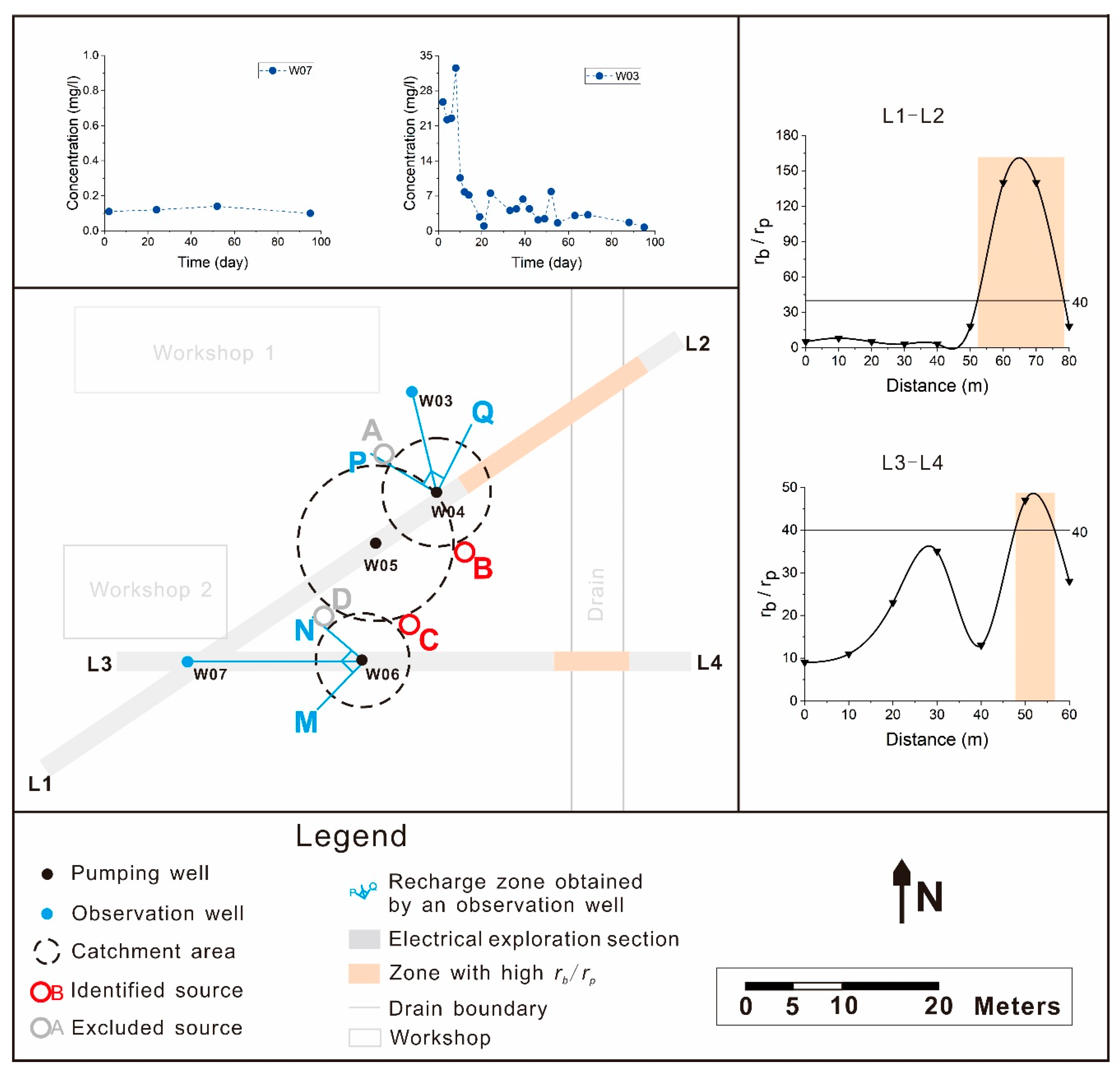
Based on the relationship between total dissolved solids and electrical resistivity, electrical prospecting sections across the high concentration zone were used to validate results indirectly. The electrical prospecting method had the advantage of continuous detection. We selected the two-way, three-stage induced polarization sounding method. The measurement electrode was deployed in the middle of the survey line. The power supply electrode supplied power in different positions. A multi-channel receiver recorded signals simultaneously when power was supplied to the electrode in different positions. The possibility of a high concentration zone was evaluated by the resistance differences between the background value obtained from outside the site (r_b) and the measured value on the line (r_p). The ratio r_b/r_p represents the relative probability of the contaminant source. The section direction was designed by identified source zone direction. Two lines of electrical prospecting were implemented to verify the identified results: Line L1-L2 crossing well W07 and W06, and Line L3-L4 crossing well W07, W05, and W04.

4. Results and Discussion

4.1. Source–Well Distance Calculation

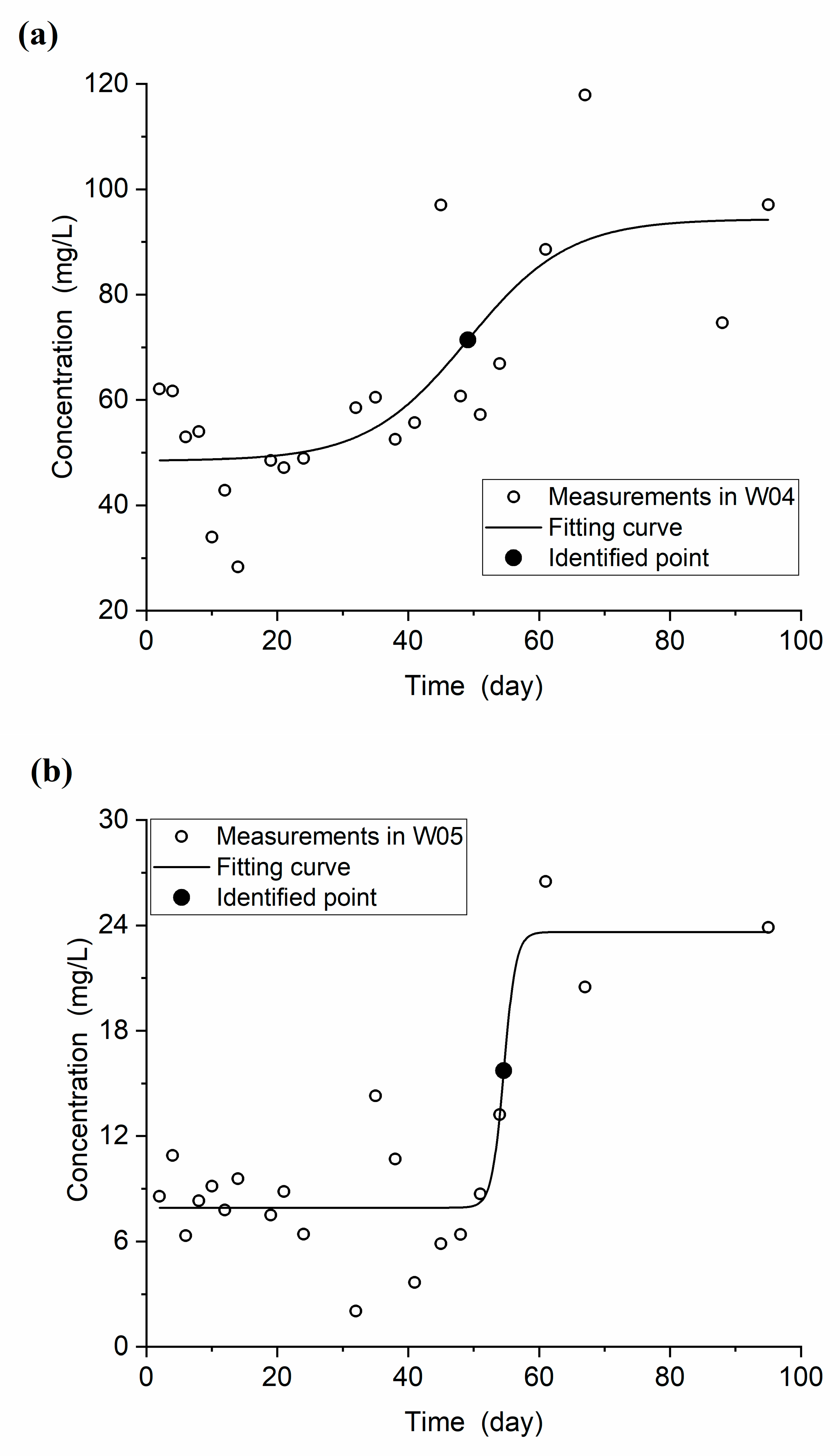
Preliminary tests indicated that the water level could reach a proximate stable condition within 24 h. During the test, concentration time series were obtained and fitted by Equation (3). Measured concentration and fitting curves are shown in Figure 4. The fitting parameters of each curve are listed in

Table 1. Fitting and calculation results of the three pumping wells.

Well	Effective Porosity (-)	Aquifer Thickness (m)	Pumping Rate (m3/day)	Retardation Factor (-)	Calculation Results
					C1 (mg/L)	C2 (mg/L)	ta (day)	l (m)	R2	lR (m)
W04	0.15	5.7	2.762	1.2	48.44	94.35	49	7	0.60	5.6
W05	0.15	5.7	5.293	1.2	7.92	23.62	55	10	0.81	8.0
W06	0.15	5.7	4.212	1.2	25.02	38.35	26	6	0.64	4.8

. The fitting of C-t series in the three pumping wells demonstrated each well was recharged by a potential source with a higher concentration than the initial value.

C-t series of pumping well W04 can be seen from Figure 4a. The initial NB concentration of well W04 under enhanced condition was 62.11 mg/L, which was the highest among the three pumping wells. According to the trend of measured sampling data, the pumping duration of well W04 could be divided into three phases. Phase one contained the period from pumping initiation to day 14; concentrations of NB in well W04 fluctuated during this stage. At day 14, the concentration of NB dropped to a minimum value of 28.29 mg/L during the whole catchment process. This stage indicated that the concentration of NB in the zone outside the steady catchment area was lower than the initial concentration of well W04. The second stage was from day 15 to day 67 of the catchment process. The concentration of NB in well W04 increased during this period. At day 48, the concentration of NB returned to the initial concentration level. From day 48 to day 67, the concentration of NB increased rapidly from 60.73 to 117.91 mg/L and reached the maximum concentration for the entire pumping duration. This rapid rise indicated the existence of a source with a higher concentration. From day 67 to the end of the test, the NB concentration in well W04 varied from 74.67 to 117.91 mg/L. Based on C-t series fitting results (Figure 4a), the t_a of well W04 was 56 days. The distance from well W04 to the potential source was 7 m as calculated by Equation (6). The calculation result considering the influence of the retardation factor l_R was 5.6 m.

Pumping well W05 was located between well W04 and W06. The initial NB concentration under enhanced condition of well W05 was 8.58 mg/L. The pumping duration of well W05 could also be divided into three phases (Figure 4b). Phase one included the first 14 days of pumping. The NB concentration varied between 6.32 and 10.90 mg/L during this phase. The second stage was from day 15 to day 61. From day 41 to day 61 in this stage, the concentration of NB in well W05 increased and reached a maximum value at day 61 of 26.50 mg/L. After day 61, the NB concentration of well W05 ranged from 20.48 to 26.50 mg/L. According to C-t series fitting results (Figure 4b), t_a of well W05 was 55 days. The distance from well W05 to the potential source was 10 m as calculated by Equation (6). The calculation result considering the influence of the retardation factor l_R was 8.0 m.

Well W06 was located to the south of well W05. C-t series of pumping well W06 can be seen in Figure 4c. The initial concentration of NB under enhanced condition was 17.01 mg/L. The concentration increased to 32.95 mg/L by day 8. NB concentration ranged from 21.57 to 28.35 mg/L between day 8 and day 24. The NB concentration in W06 increased rapidly from day 24 to day 32. On day 32, the concentration of NB reached 50.89 mg/L, which was the maximum concentration of well W06 during the pumping process. After day 32, the concentration of NB decreased slowly to 27.12 mg/L. According to C-t series fitting results (Figure 4c), t_a of well W06 was 30 days. The distance from well W06 to potential source was 6 m as calculated by Equation (6). The calculation result considering the influence of the retardation factor l_R was 4.8 m.

4.2. Source Zone Localization and Verification

The catchment area using l_R as the radius of each pumping well is shown in Figure 5. Four position points of a potential source (A, B, C, and D) were obtained through intersections of three circles. The initial NB concentration of well W04 was the highest of the wells and it was likely closest to the unknown source. Position points A and B were identified by well W04 and W05. Observation well W03 was located northwest of W04. In the local source–sink relationship, groundwater transport was from the direction of well W03 to well W04. According to the measured concentration in the observation well W03 during the pumping process, the groundwater that recharged well W03 was slightly polluted. The low concentration recharge caused a sharp concentration fall for W03 by the pumping of wells W04 and W05. Therefore, the direction of arc P-Q was excluded from the potential sources of well W04. Position point A, located between arc P-Q, was removed from the potential sources. This indicated that workshop 1 was not the source location of NB. Position point B was the probable high concentration source recharge for well W04. Compared with the former operation of this site, point B was located close to the drain that collected the wastewater of this factory according to the production history.

Position points C and D were the potential sources identified by wells W05 and W06. The closed observation well W07 was sampled during the pumping process. The sampling results indicated that the concentrations were maintained at a lower level than that of well W06. This revealed that the concentration of recharge water from the direction of W07 was much lower than W06. Therefore, the direction of arc M-N was excluded from the potential source direction of well W06. Point D, located between arc M-N, was removed from the potential sources. This indicated that workshop 2 was not the location for the release of NB. Point C was identified as a likely NB source. Both position points B and C indicated that the drain was the most likely release position of a high concentration of NB. A ranked list of the possible positions of sources is shown in

Table 2. Ranked list of potential source position.

Identified Source Position	Based Wells	Source Priority	Next Step
A	W04, W05, W03	Low	Monitoring
B	W04, W05	High	First remediation
C	W05, W06	Middle	Further investigation
D	W05, W06, W07	Low	Monitoring

.

The results of the electrical prospecting are labeled in Figure 5. The area with a high ratio of r_b/r_p demonstrated that the zone near the drain was a high level of overall pollution. We compared the identified source position with the high rate of r_b/r_p on the electrical prospecting lines. Point B matched well with the high rate of r_b/r_p of line L1-L2. The northeast position of W04 (Q-B) was identified as a heavily polluted area (potential source). This needs to be confirmed first with further investigation and in the remediation phase. The high rate of r_b/r_p on line L1-L2 (about 180) was much higher than the value of line L3-L4 (about 50), which indicates that the total magnitude of the source that recharges well W04 (Q-B) was much higher than that of well W06 (C-M).

4.3. Restrictions of Method Application

The characteristics of groundwater flow and solute transport in low-permeability aquifers indicates that the range of pollution plumes formed by point sources is small. It needs a large number of intensive monitoring points to obtain source location in groundwater. At the initial stage of the investigation, there are insufficient monitoring points within the site. The source identification method established in this paper can use limited monitoring wells to help determine the source of pollution. However, the developed method of identifying pollution sources is currently only applicable to simple scenarios. The method has following limitations when it is used on the actual site.

This method adopts the strategy of artificial intensification. In order to form a continuous enhanced groundwater flow, the “low permeability” aquifer targeted in this paper is an aquifer with a hydraulic conductivity between 1 × 10⁻⁶ and 1 × 10⁻⁵ m/s. For highly permeable aquifers (hydraulic conductivity is higher than 1 × 10⁻⁴ m/s), analysis based on sampling points makes it easy to identify contaminated plumes without the need for additional reinforcement. In extremely low permeability aquifers (hydraulic conductivity is lower than 1 × 10⁻⁷ m/s), such as thick homogeneous clay layers, even under artificially strengthened conditions, it is not possible to form continuous groundwater flow.

In addition, during artificial enhancement, only convection migration is considered and therefore only pollutants with the same transport characteristics as groundwater are suitable for this method. The approach is applicable to conservative solutes, or other contaminants that can be treated as conservative during the artificial enhancement. The distance l may be overstated for sorption, retardation, and reactive transport. For these types of contaminants, another associated tracing index should be obtained to describe the migration process. Besides, dispersion also affects the curve characteristics of the concentration time series.

Another aspect is that the method is restricted to homogeneous aquifers. In the actual site, even if the aquifer is homogeneous as a whole, the local extremely low permeability lens will affect groundwater flow and solute transport. The trend difference of the three curves in Figure 4 indicates that the aquifer medium may have a local heterogeneous lens. Influence in this respect is ignored in this method. Moreover, only horizontal flow of groundwater is considered. Pumping and observation wells used in this method should be over the full depth of the aquifer. The method assumes perfect vertical mixing in the aquifer, while this assumption is not valid close to the source.

The uncertainty of this method is due to aquifer conditions and pollution history. There are uncertainties in the characterization of aquifer parameters such as aquifer thickness and effective porosity. Besides, there are also uncertainties of numbers, release history, and existence of the form of the source. In order to improve the accuracy of the method in field applications, the method conceptual model and site hydrological conditions need to be optimized in further study. Furthermore, it is necessary to compare it with other source identification methods in terms of time, cost, and accuracy.

5. Conclusions

A source zone localization method is developed in this study that adopts the strategy of an artificially enhanced catchment. The distance from a pumping well to the potential source zone is calculated by integrating C-t series curve fitting and radial well flow. The source position is determined by the distance intersection using catchment areas obtained from multiple pumping wells. The method is restricted to an approximately homogeneous aquifer with average hydraulic conductivity ranging from 1 × 10⁻⁶ to 1 × 10⁻⁵ m/s. This method is applicable to target contaminants whose transport process can be generalized to convective migration. This method was applied in an industrial site located in the coastal area of the North China Plain. A 95-day field test using artificial disturbance of three pumping wells identified the pollution source position close to a waste drain. The obtained zone should be treated first in a future remediation process. Field application results and their verification indicate that this new method can be used to identify pollution sources in these types of contaminated sites. The sampling schedule and pumping well position should be optimized to improve the accuracy of identification in future research.