Long-Term Trends in 20-Day Cumulative Precipitation for Residential Rainwater Harvesting in Poland

Abstract

Rainwater harvesting (RWH) for domestic uses is widely regarded as an economic and ecological solution in water conservation and storm management programs. This paper aims at evaluating long-term trends in 20-day cumulative rainfall periods per year in Poland, for assessing its impact on the design and operation conditions for RWH systems and resource availability. The time-series employed corresponds to a set of 50-year long time-series of rainfall (from 1970 to 2019) recorded at 19 synoptic meteorological stations scattered across Poland, one of the European countries with the lowest water availability index. The methods employed for assessing trends were the Mann–Kendall test (M–K) and the Sen’s slope estimator. Most of the datasets exhibit stationary behaviour during the 50-year long period, however, statistically significant downward trends were detected for precipitations in Wrocław and Opole. The findings of this study are valuable assets for integrated water management and sustainable planning in Poland.

1. Introduction

As in many areas across the world, Poland is currently experiencing a deficit in water resources. The freshwater resources per capita have decreased from an average of 1839.3 m³ (for the period 1946–2011) to less than 1600 m³ [1]. This water availability index for Poland is almost three times lower than the European average (4800 m³ per capita) and nearly four times smaller than the world’s average (6000 m³ per capita) [2], making Poland one of the countries with fewer water resources in Europe [3,4].

According to Orlińska-Woźniak et al. [5,6], the leading causes of this situation are both adverse climatic and hydrological conditions, as well as a robust socio-economic development in Poland, observed in recent decades. The topographic, geological and meteorological features of the area, as well as land use, influence the distribution and size of surface water, groundwater, and rainwater resources [5]. Atmospheric precipitation is the primary source of Polish water resources, so they largely determine the renewable nature of water resources, characterised by a considerable time and spatial variability. The average annual rainfall in lowland areas is 450–650 mm, while in the mountain areas annual this parameter reaches more than 1000 mm. While mountain and foothill areas are relatively abundant in water, shortages of this resource are already occurring in the lowlands [7]. As for the average monthly precipitations, the lowest values correspond to the winter months from December to February (an average of 34.9 mm/month) and the highest occurring in the summer months from June to August (an average of 73.4 mm/month). This distribution is characteristic of Poland’s climatic zone. The annual cycle of precipitation phenomena determines the average annual variability of surface run-off. The total running waters resources of Poland are about 62 km³, based on the average between 1951 and 2005, but it should be noted that there is a higher frequency of extended low streamflow periods when compared to high streamflow periods [8].

The state of water resources is one of the main concerns related to climate change, as progressive global warming alters the water cycle [9]. In the coming decades, Poland faces the threat of water shortages and a decrease in the national surface and groundwater resources, and it is anticipated that extreme hydrological phenomena (both drought and floods) might increase as a result of climate change [10]. There is evidence that severe water deficits and excesses can occur in the same area over a single season. For instance, in July 1997, heavy rainfalls that caused violent floods were followed by an abnormally dry period across a significant part of Poland. Another example was the summer of 2006 when a period of heavy rainfalls was immediately followed by a severe drought [11].

Within this context, increasing awareness about this situation has led to individual and institutional actions to save and protect water resources around the world include promoting the sustainable use and management of water resources, reducing water losses in supply systems, and searching for alternative freshwater sources [12]. In water supply systems, one of the main objectives is reducing the water losses by preventing failures in water intakes and networks. Consequently, integrated water management systems employ the support of advanced computer models and artificial neural networks to achieve this goal [13,14,15]. The rainwater harvesting (RWH) is promoted as a widely available, alternative source of water for an entire range of uses, including household purposes, and its implementation in residential buildings are regarded as economically and ecologically beneficial, as long as adequate maintenance and operation are guaranteed [16]. The use of rainwater for replacing the tap water for indoor and outdoor demands reduces pressure on water supply systems and water intakes [17]. On a large scale, RWH reduces the energy demand employed for raw water intake, pumping and treatment in water supply systems; and it also relieves sewage systems and reduces the risk of local floods, as it favours local rainfall retention [18,19,20]. These are attractive features for water supply and wastewater management systems operators.

The law in Poland prohibits the discharge of rainwater and drainage water into the sanitary sewage system. Water supply companies carry out intensified inspections in this area. To promote rainwater harvesting as complementary technology, in June 2020 the Polish Ministry of Climate and the National Fund for Environmental Protection and Water Management announced the “My Water” programme. It will be implemented in the years 2020–2024. Twenty thousand home installations are to be built to manage rainwater and snowmelt on the property. It is estimated that the house investments will retain 1 million m³ of water annually at the place of rainfall on private plots.

The RWH reliability requires considering quantitative and qualitative criteria, expressed through the system sizing and water quality parameters. The primary task is to efficiently collect rainfall and securely store the precipitation for later in-situ use, to guarantee the quality and quantity of the harvested rainwater for the allowing the maximum possible replacement of tap water [21].

Regular residential water requirements include cooking, cleaning, dishwashing, garden watering, laundry, showers, baths and toilet flushing (Figure 1). Depending on the quality standards met, a rainwater harvesting system can provide up to 100% of the tap water needs in the household. According to European statutes, if the RWH system provides water that meets bathing quality, it can replace over 50% of total tap water demand, and if drinking water quality is achieved, it can be safely used for all household purposes, even as the single water source of the dwelling place [22,23].

The use of rainwater in households requires meeting physicochemical and microbiological water quality standards, such as those defined in the European Water Directives. The Bathing Water Directive provides quality standards of public freshwater bathing areas (e.g., rivers or lakes), to safeguard public health and protect the aquatic environment. [22]. The Drinking Water Directive concerns the quality of water intended for human consumption, to protect human health from adverse effects of any contamination [23]. The quality of the collected rainwater depends on the cleanness of the conveying system, atmospheric contamination, the storage conditions and the filtering and treatment processes applied in the RWH system. The stages of passing through the atmosphere and flowing down the catchment determine the rainwater composition, which is affected both by local and long-distance transported dust and aerosols of natural and anthropogenic origin [24,25,26,27,28]. The regional distribution of precipitation also influences the pollution of run-offs. The longer the dry periods between rainfall, the rainfall flushes away more accumulated pollutants from the roof. The first flush rainfall volume should therefore be diverted from the tank to avoid pollution from roof runoff [29]. Frequent, long-lasting, and moderate precipitations are associated with a better quality of collected rainwater. Many studies conducted over the last two decades [30,31,32,33,34,35,36,37,38] confirm that water from RWH systems can be successfully used (excluding first flush) for household purposes, both indoors and outdoors. The physicochemical and microbiological composition of supplied rainwater is suitable for animals and plants, as well as for cleaning and washing purposes.

The technical factors that determine the RWH system design for residential buildings are water volume requirements, rainfall distribution along the year, type and size of the catchment, and rainfall data (Figure 2). As the system layout remains constant for the lifetime of the RWH system, its performance is defined by the precipitation regime, climate variability and long-term trends observed in rainfall [21].

The rainfall regime heavily affects both the freshwater resources availability and RWH design and operation. At the same time, RWH systems help to reduce the burden on limited freshwater resources, as in the Poland case. Sustainable and efficient use of rainwater on a national scale requires evaluation of occurrence and behaviour of local rainfall, even more in the context of global warming and climate change [39], as well as a lot of local buy-in and coordination. Therefore, this paper aims at analysing long-term trends in precipitation in Poland, for assessing its impact on the design and operation conditions for RWH systems and resource availability.

2. Materials and Methods

2.1. Rainfall Data

The rainfall pattern is the main indicator of household rainwater harvesting potential in Poland. This paper analyses a set of 50-year long time-series of daily rainfall (from 1970 to 2019) at 19 Polish cities. The daily time step was chosen due to the very long simulation period and the national scale of the research, although it is known that more accurate results are obtained for continuous simulation [40]. The primary source of precipitation data are the records by meteorological stations managed by the Institute of Meteorology and Water Management—National Research Institute (IMWM-NRI) [41], located in major Polish cities: Białystok, Suwałki, Olsztyn, Gdańsk, Koszalin, Szczecin, Toruń, Poznań, Gorzów Wielkopolski, Zielona Góra, Wrocław, Opole, Katowice, Kraków, Rzeszów, Kielce, Lublin, Łódź and Warsaw (Figure 3). Verified daily rainfall data come from synoptic stations, which are the highest order meteorological station type in Poland. These stations are linked with the World Meteorological Organization (WMO) observing and prediction system called World Weather Watch (WWW) as well as with the European Flood Awareness System (EFAS). The use of these two sources guarantees the quality and completeness of measurement data over the 50 years employed for this analysis.

The authors assumed that IMWM-NRI precipitation data recording methods employed for time-series used in this study were homogeneous and robust. Moreover, the vast majority of these meteorological stations were tested by Pińskwar et al. [42] for homogeneity tests of the rainfall time-series (Mann–Whitney–Pettitt test, Penalised maximal t-test and the Standard Normal homogeneity test (SNHT) for single series), which indicated the adequacy of these data for statistical analysis, except for the Racibórz and Śnieżka stations, both excluded in the present study.

The WMO recommends using a long-term period for statistical analysis of meteorological variables [39], with a minimum of 30 years of multi-year data for determining climatological standards. A more extended period of measurements is taken into account if the analysis aims at evaluating the variability in time of a climate variable. Some authors have conducted recent studies for Poland assessing time-series longer than 30 years. Pińskwar et al. [42] analysed changes in extreme precipitation in Poland, for the period 1951–2015. Similarly, Lupikasza [43] conducted trend detection tests to study the spatial and temporal variability of extreme rainfalls in Poland for the period 1951–2006. Kaźmierczak et al. [44] evaluated trends in rainfall for Wrocław in the years 1961–2017, finding a statistically significant decreasing trend for moderately intense precipitations. Urban et al. [45] examined the variability of snow cover in the Polish and Czech Western Sudeten Mountains, in the years 1961–2015.

Figure 3 also depicts the spatial variability of the average multi-annual rainfall in Poland. The occurrence of high rainfall values in the foothill areas is a characteristic of the continental climate of Poland, as represented by meteorological stations in the south of the country such as Rzeszów, Kraków, Katowice or Wrocław. Additionally, relatively low annual rainfall occurs in the central part of the country, in the lowland belt covering towns from Szczecin to Lublin, while the highest magnitudes occurs on the western portion of Baltic coast and the Tatras mountain area (over 1000 mm per year). Annual precipitation amounts of eastern portion of Baltic coast is characterised as low. The average annual precipitation (from 1970 to 2019) in the analysed cities is 597.3 mm. Among the cities analysed in the study, the lowest average annual precipitation occurs in Gdańsk (512.7 mm) and Poznań (518.1 mm), and the highest in Koszalin (731.6 mm) and Katowice (724.6 mm).

Figure 4 shows that the highest average monthly rainfall occurs in the summer season, from May (V) to October (X), and within a range from 50 to 80 mm. In winter, especially from December (XII) to February (II), most precipitation occurs as rain-on-snow or snow (about 20–40 mm monthly). Generally, for all the months over the long-time period under analysis, the annual highest magnitudes of average monthly precipitation were recorded in Koszalin, Katowice or Kraków. In contrast, the annual lowest magnitude precipitations occur in Gdańsk, Poznań, Szczecin, Gorzów Wielkopolski, Zielona Góra or Wrocław.

2.2. Rainwater Storage Period and Tank Capacity

This paper presents a general model for analysing residential RWH systems to assess the impact of rainfall patterns on the reliability of such systems in Poland. The recommended storage period for rainwater for individual RWH systems is 2–3 weeks, with the possibility of safe prolongation up to 4 weeks [46]. The analysis assumes a typical water storage period of 20 days, in which the rainwater tank capacity allows it to meet the indoor rainwater requirements. The study included four sizes of households with the same catchment area and different rainwater demand profiles, where 20-day rainwater supply will be provided by tanks with storage capacities of 1.0, 2.0, 3.0 and 4.0 m³ (

Table 1. Determining factors of four analysed cases of residential RWH system.

	Household 1	Household 2	Household 3	Household 4
20-day rainwater demand	1000 dm3	2000 dm3	3000 dm3	4000 dm3
Catchment area (roof)	125 m2	125 m2	125 m2	125 m2
Storage capacity (tank)	1.0 m3	2.0 m3	3.0 m3	4.0 m3

). Filling such tanks requires between 10 and 40 mm of total precipitation, considering a 125 m² catchment area (a typical roof size in Poland) with a 0.8 run-off factor for typical conditions (20% water loss). The first flush volume has been neglected to simplify the calculation.

Figure 5 graphically shows the water balance model for analysing an RWH system during a 20-day storage period. The working fields of 1.0, 2.0, 3.0 and 4.0 m³ storage capacities were marked in four shades of blue. The graph illustrates the basic principles of the analysis and at the same time allows to quickly determine the amount of rainwater delivered during 20 days from a tank with a specific capacity and for a particular 20-day cumulative rainfall.

For example, for a 20-day cumulative rainfall of 5 mm, RWH systems with tanks of all analysed capacities will be able to collect and provide 500 dm³ of rainwater for use in the household (case A). These savings correspond to 500 dm³ of tap water, e.g., for flushing toilets or washing within the typical storage period of 20 days. When the 20-day cumulative rainfall is 15 mm, a 1.0 m³ tank will not be able to store all the available rain, but it will provide the 1000 dm³ of rainwater corresponding to its capacity (case B), which fully satisfies the rainwater demand in a building with an RWH system of this size during the typical storage period. Accordingly, larger harvesting systems (2.0, 3.0 and 4.0 m³) would accumulate this entire rainfall and provide 1500 dm³ of rainwater, but it will not fill the tanks, and it will not cover the total rainwater requirements either, meaning that these RWH systems would require supplementing the demand with tap water (case C). For a 20-day cumulative rainfall of 35 mm, the run-off would fill and exceed the capacity of the tanks up to 3.0 m³. In these cases, the rainwater will meet and cover the local 20-day water requirements. The 4.0 m³ RWH system, with a rainwater demand of 4000 dm³, will collect and supply only 3500 dm³ of rainwater, which requires partial reliance on tap water to meet the requirements. (case D). Based on the previous considerations, the overflows are a loss of resources for RWH systems, while on the other hand, insufficient rainwater translates into costs associated with consuming tap water. Therefore, the magnitude of the 20-day cumulative precipitations, along with the stochastic nature of rainfall, determines the working conditions of the RWH systems. The proposed 20-day water balance model was used to analyse the long-term impact of 50-year rainfall time series on RWH reliability in 19 Polish cities.

This study analyses the 20-day cumulative rainfalls above 10, 20, 30 and 40 mm, which correspond to the assumptions made for filling tanks with volumes of 1.0, 2.0, 3.0 and 4.0 m³. Additionally, precipitations in the range of [0–10), [10–20), [20–30) and [30–40) mm are analysed to show the intermediate operating states of the RWH systems when 20-day water demand is partially covered by rainwater and completed with tap water. The assessment also includes statistical distributions of operational RWH parameters, potential and pattern of precipitation and their 50-year change trends at 19 cities in Poland.

2.3. Research Methods

There are several statistical tests for detecting trends in hydrological time-series (e.g., linear regression test, the Mann–Kendall test (M–K), and the Spearman’s rho test). This research employs the non-parametric M–K test, widely applied in hydrological studies [47,48,49,50,51], mostly because M–K does not require normally distributed data and it has low sensitivity to outliers, in this case, extreme meteorological phenomena such as floods or droughts.

This test uses rank correlation statistics to answer the question as to whether the values measured in the time series present a statistically significant increasing or decreasing trend. The M–K test analyses the sign of the difference between successive elements of the time series X_t, given as $x_1\le x_2\le \dots \le x_t$, where each new value is compared to all previously measured values [52,53], and $t$ stands for time unit $t=1, 2,\dots , 50$. The following equation calculates the statistic $S$:

$$S={\displaystyle \sum }_{i=1}^{n-1}{\displaystyle \sum }_{j=i+1}^{n}sign\left(x_j-x_i\right)$$

(1)

where the indexes j and i emphasise all possible pairs composed of earlier and later values of a deseasonalised (e.g., annual) series X_t. By substituting $x_j-x_i=\theta$ we get:

$$sign\left(\theta \right)=\{\begin{array}{c}+1 for \theta >0\\ 0 for \theta =0\\ -1 for \theta <0\end{array}$$

(2)

where $sign\left(\theta \right)$ is the is the positive or negative sign of the parenthetical result.

To indicate the direction of a trend and its statistical significance, the sign of the S statistic, the Sen’s slope estimator and the confidence level magnitudes should be determined. If the statistic $S$ is positive, the more recent measurements are higher than the previous, indicating an upward trend in the measured values. If S is negative, there is a downward trend.

The rate of the change of the analysed trend in time can be described by the directional coefficient of the straight line expressed by Sen’s slope estimator $\beta$ (also called Theil-Sen slope estimator), which is commonly used to detect the magnitude of trends in univariate time series. It can be defined as the median value of all the slopes given by all the possible pairs among data forming the time series $X_t$:

$$\beta =median\left(\frac{x_j-x_i}{j-i}\right)$$

(3)

calculated for every $i<j$, where $i=1, 2, \dots , n-1$ and $j=2, 3, \dots , n$. The calculation of the intercept parameter $y_S$ can be used to construct the trend lines in plots of this type of slope. Following [54,55], $y_S$ can be computed as:

$$y_S=X_t-\beta t$$

(4)

with $t$ and $\beta$ indicating the element of the time-series and Sen’s slope, respectively.

According to [54,56], the null hypothesis is the absence of trend ($H_0:\beta =0$) and the alternative hypothesis is that a statistically significant trend is detected ($H_1:\beta \ne 0$), considering statistically significant changes above a confidence level of 95% [57]. For this paper, the confidence level index ($CLI$) ranging from 90 to 95% is assumed to be close to statistical significance, whereas the magnitudes of $CLI$ between 75 and 90% directly indicates a tendency to change. Based on the considerations by [42], all investigated changes below the confidence level of 75% are considered as irrelevant and without a specific direction of change.

According to Wagesho et al. [57], the theoretical lower ($LCL$) and upper ($UCL$) confidence limits of the Theil-Sen slope can be calculated as:

$$LCL=\frac{t_i-Z_{1-\alpha /2}\sqrt{Var\left(S\right)}}{2}$$

(5)

$$UCL=\frac{t_i+Z_{1-\alpha /2}\sqrt{Var\left(S\right)}}{2}$$

(6)

where $t_i$ stands for the number of data points (observations) in the i-th data pairs (also called tied data) of analyzed data set and $Z_{1-\alpha /2}$ is the ($1-\alpha /2$) value of the normal distribution, whereas for two-sided (upper and lower bound) the magnitude of 95% ($\alpha =0.05$) confidence limit of the corresponding $Z_{1-\alpha /2}=1.96$.

For independent and identically distributed data, the S mean is E(S) = 0, and the sample variance $Var\left(S\right)$ is given by:

$$Var\left(S\right)=\frac{n\left(n-1\right)\left(2n+5\right)-{{\displaystyle \sum }}_{i=1}^m{t}_i\left(i-1\right)\left(2i+5\right)}{18}$$

(7)

where m is the number of the tied groups in the data set of extent $i$. For example, in the eight element sequence of measurements given by $t_i\in \left\{15, 14, 11, 11, 14, 14, 11, 15\right\}$ m = 3 denotes tied groups, for which t₁ = 2 for the tied value 15, t₂ = 3 for the tied value 14, and t₃ = 3 for the tied value 11.

3. Results

3.1. Precipitation Potential

First, the annual occurrence of 20-day cumulative rainfall higher than 10, 20, 30 and 40 mm in the 19 analysed cities was examined. The results of the analyses, as the percentage share in the year of periods with 20-day rainfall sums exceeding the preset amount, are summarised in

Table 2. Twenty-day cumulative rainfall for set thresholds—percentage share in the year.

City	Total Rainfall				Total Rainfall				Total Rainfall				Total Rainfall
	≥10 mm				≥20 mm				≥30 mm				≥40 mm
	Min	Mean	Max	SD	Min	Mean	Max	SD	Min	Mean	Max	SD	Min	Mean	Max	SD
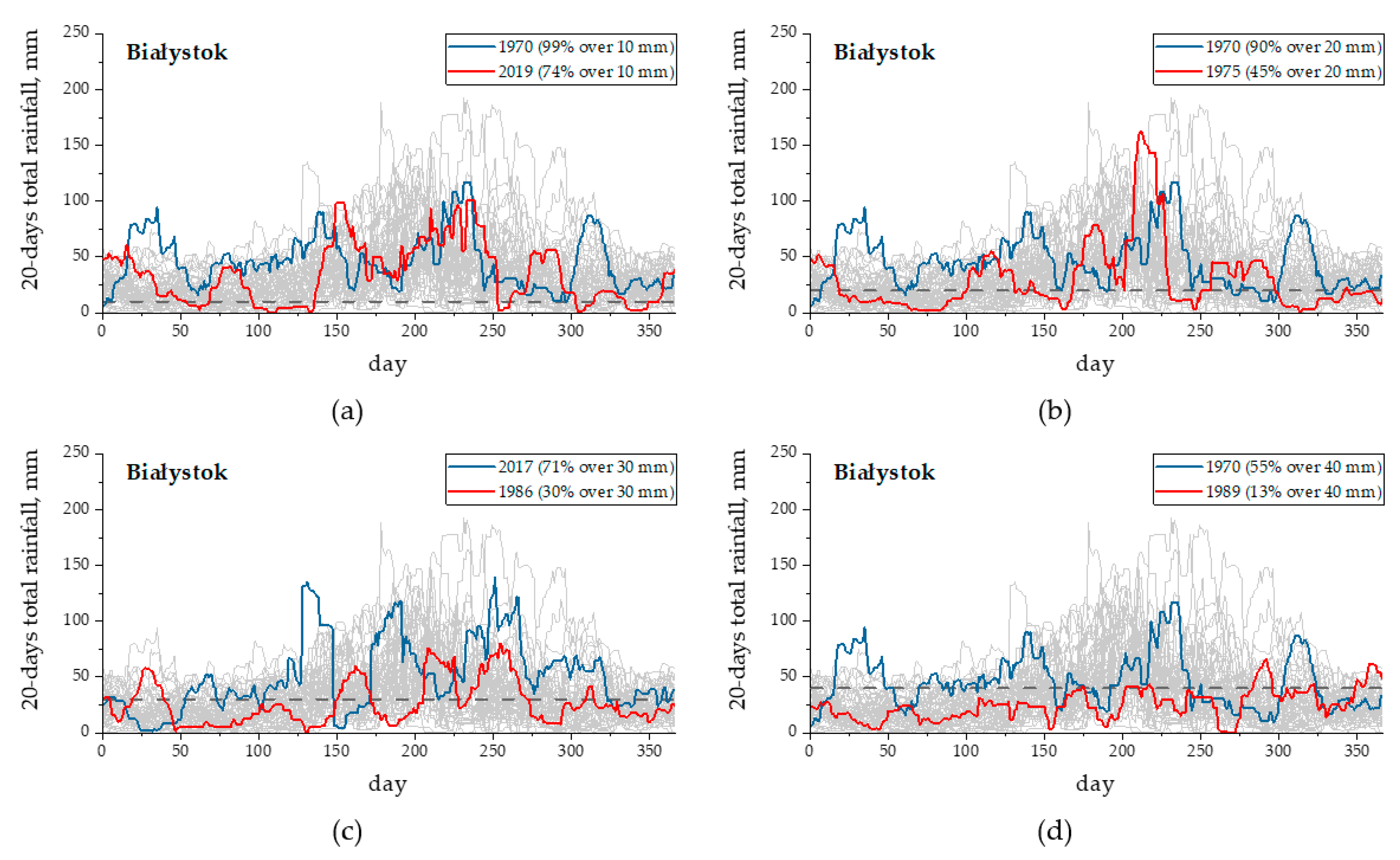
Białystok	74%	86%	99%	7%	45%	65%	90%	9%	30%	45%	71%	9%	13%	30%	55%	9%
Gdańsk	52%	79%	98%	9%	30%	54%	83%	11%	16%	35%	58%	10%	7%	23%	43%	8%
Gorzów Wlkp.	68%	84%	95%	7%	35%	61%	86%	11%	13%	41%	66%	12%	5%	26%	45%	10%
Katowice	73%	90%	98%	6%	58%	74%	87%	8%	35%	56%	75%	10%	16%	40%	58%	10%
Kielce	67%	86%	100%	7%	47%	67%	95%	9%	24%	46%	68%	9%	12%	30%	44%	8%
Koszalin	71%	89%	99%	6%	43%	73%	91%	9%	31%	56%	77%	10%	19%	41%	67%	11%
Kraków	72%	88%	98%	6%	47%	69%	85%	9%	30%	49%	67%	9%	14%	33%	52%	8%
Lublin	66%	84%	96%	7%	39%	63%	84%	9%	23%	42%	62%	9%	5%	28%	43%	9%
Łódź	69%	85%	97%	7%	47%	64%	86%	9%	26%	43%	72%	10%	7%	27%	51%	9%
Olsztyn	73%	88%	99%	6%	41%	68%	91%	10%	21%	49%	71%	10%	11%	34%	55%	10%
Opole	69%	85%	97%	7%	37%	65%	86%	10%	19%	45%	66%	11%	5%	30%	50%	9%
Poznań	64%	82%	94%	9%	33%	58%	80%	12%	9%	35%	57%	12%	1%	22%	40%	10%
Rzeszów	67%	87%	99%	7%	34%	66%	84%	11%	15%	46%	68%	11%	9%	32%	50%	10%
Suwałki	75%	87%	98%	6%	49%	66%	83%	9%	29%	47%	73%	8%	15%	31%	54%	8%
Szczecin	59%	84%	98%	8%	39%	63%	85%	10%	14%	41%	66%	11%	5%	27%	47%	9%
Toruń	63%	83%	98%	8%	31%	58%	77%	10%	8%	37%	56%	11%	0%	23%	43%	9%
Warsaw	65%	82%	95%	8%	43%	59%	81%	9%	23%	37%	63%	9%	5%	24%	42%	8%
Wrocław	67%	83%	95%	7%	41%	59%	77%	8%	20%	39%	56%	9%	12%	26%	46%	8%
Zielona Góra	70%	85%	96%	6%	40%	64%	83%	9%	22%	44%	63%	10%	7%	27%	50%	10%

.

Using Bialystok as an example, the percentage duration during the year of periods with 20-day cumulative rainfall exceeding 10 mm averaged 86% (during the 50 years), with a minimum value of 74% observed in 2019 and a maximum value of 99% in 1970. A 20-day cumulative rainfall of at least 10 mm allows filling a tank with a volume of 1 m³ under the assumed conditions (Figure 5). For cumulative precipitation exceeding 20 mm, the annual average percentage for this period is 65%, with values ranging from 45% (for 1975) to 90% (for 1970). Similarly, the average annual duration of periods with 20-day cumulative rainfall exceeding 30 mm falls to 45%, with a minimum value of 30% (for 1986) and a maximum of 71% (for 2017). Twenty-day cumulative rainfall exceeding 40 mm occurred on average 30% of the year, with a minimum of only 13% recorded in 1989 and a maximum of 55% in 1970, with this 20-day cumulative of 40 mm allowing to fill a 4 m³ tank, as shown in Figure 5. Figure 6 presents the behaviour of the 20-day cumulative rainfall described for Białystok over the years 1970–2019. The dashed line marks the corresponding thresholds of 10, 20, 30 and 40 mm, the blue line marks the year with the most extended duration of states with the sum above the dashed line, while the red line marks the year with the shortest total duration of these states.

Similar results occurred in the remaining 18 analysed cities. The annual average percentage of 20-day periods with cumulative rainfall exceeding 10 mm ranged from 79% for Gdańsk to 89% for Koszalin. For this threshold, the maximum observed in Kielce is worth noting, which was as much as 100% in 1970. For periods with totals exceeding 20 mm, the average share in the year of these periods oscillated between 54% in Gdańsk to 74% in Katowice. For the threshold of 30 mm cumulative rainfall, the annual average ranged from 35% for Gdańsk and Poznań to 56% for Katowice and Koszalin. For the highest threshold value (for rainfall totals exceeding 40 mm), the minimum annual average of 20-day periods occurred for Poznań (21%) and the maximum for Koszalin (41%).

The annual fraction with 20-day cumulative rainfalls according to the class intervals of [0–10) mm, [10–20) mm, [20–30) mm, and [30–40) mm was calculated and summarised in

Table 3. Twenty-day cumulative rainfall for the analysed intervals—percentage share in the year.

City	Total Rainfall				Total Rainfall				Total Rainfall				Total Rainfall
	[0–10) mm				[10–20) mm				[20–30) mm				[30–40) mm
	Min	Mean	Max	SD	Min	Mean	Max	SD	Min	Mean	Max	SD	Min	Mean	Max	SD
Białystok	1%	14%	26%	7%	5%	21%	34%	6%	6%	20%	31%	5%	7%	15%	30%	5%
Gdańsk	2%	21%	48%	9%	12%	25%	42%	6%	8%	19%	30%	5%	2%	12%	25%	5%
Gorzów Wlkp.	5%	16%	32%	7%	9%	23%	39%	8%	11%	20%	32%	5%	6%	15%	23%	4%
Katowice	2%	10%	27%	6%	5%	16%	30%	5%	10%	18%	28%	5%	6%	16%	27%	5%
Kielce	0%	14%	33%	7%	5%	19%	31%	6%	11%	21%	33%	5%	6%	16%	30%	5%
Koszalin	1%	11%	29%	6%	7%	16%	34%	5%	9%	17%	28%	5%	6%	15%	23%	4%
Kraków	2%	12%	28%	6%	6%	19%	35%	6%	9%	20%	33%	6%	6%	16%	25%	5%
Lublin	4%	16%	34%	7%	11%	22%	35%	6%	10%	20%	34%	5%	6%	15%	24%	4%
Łódź	3%	15%	31%	7%	6%	21%	31%	6%	9%	22%	31%	5%	5%	16%	28%	5%
Olsztyn	1%	12%	27%	6%	6%	20%	39%	7%	9%	19%	28%	5%	5%	15%	26%	4%
Opole	3%	15%	31%	7%	8%	21%	40%	7%	8%	20%	32%	6%	7%	14%	27%	5%
Poznań	6%	18%	36%	9%	13%	25%	37%	6%	11%	22%	34%	5%	2%	14%	25%	6%
Rzeszów	1%	13%	33%	7%	9%	21%	44%	7%	9%	20%	36%	6%	6%	14%	25%	5%
Suwałki	2%	13%	25%	6%	5%	21%	39%	6%	6%	19%	30%	6%	8%	16%	26%	4%
Szczecin	2%	16%	41%	8%	8%	21%	34%	6%	9%	21%	36%	6%	7%	15%	25%	4%
Toruń	2%	17%	37%	8%	10%	25%	52%	8%	11%	21%	34%	5%	6%	14%	23%	4%
Warsaw	5%	18%	35%	8%	11%	24%	39%	7%	9%	21%	35%	5%	5%	14%	28%	4%
Wrocław	5%	17%	33%	7%	10%	24%	42%	8%	9%	19%	30%	5%	1%	14%	27%	5%
Zielona Góra	4%	15%	30%	6%	9%	21%	38%	6%	11%	20%	35%	5%	7%	17%	27%	5%

.

The annual average frequency of periods with a 20-day cumulative rain between [0–10) mm ranged from 10% for Katowice to 21% for Gdańsk. In the case of the interval between [10–20) mm, the smallest average found was 16% (Katowice and Koszalin), while a highest equal to 25% found in three cities: Gdańsk, Poznań and Toruń. For the interval between [20–30) mm, the average fraction of the year ranged from 17% (Koszalin) to 22% (Łódź and Poznań). Zielona Góra registers the highest average fraction of the year with 20-day cumulative rainfall ranging [30–40) mm (17%), and the smallest occurs in Gdańsk (12%).

3.2. Trends of Change

Significant changes in the behaviour of the rainfall regime might have an impact on the operating conditions of the RWH systems. Therefore, this paper assesses the existence of trends in the precipitation time-series in the 19 meteorological stations analysed for the period 1970–2019, using the M–K test for this purpose.

Table 4. Trend detection parameters for 20-day cumulative rainfall for the different thresholds under study, during the period 1970–2019.

City	Cumulative 20-Day Rainfall ≥10 mm			Cumulative 20-Day Rainfall ≥20 mm			Cumulative 20-Day Rainfall ≥30 mm			Cumulative 20-Day Rainfall ≥40 mm
	$\mathit{S}$	$\mathit{\beta }$(%)	$\mathit{C}\mathit{L}\mathit{I}$	$\mathit{S}$	$\mathit{\beta }$(%)	$\mathit{C}\mathit{L}\mathit{I}$	$\mathit{S}$	$\mathit{\beta }$(%)	$\mathit{C}\mathit{L}\mathit{I}$	$\mathit{S}$	$\mathit{\beta }$(%)	$\mathit{C}\mathit{L}\mathit{I}$
Białystok	39	0.04	25%	91	0.09	55%	178	0.13	86%	36	0.03	23%
Gdańsk	−24	−0.02	15%	−72	−0.07	45%	−170	−0.15	84%	−125	−0.10	70%
Gorzów Wlkp.	124	0.07	70%	94	0.09	56%	98	0.12	58%	32	0.03	20%
Katowice	2	0.00	1%	−67	−0.05	42%	−151	−0.09	79%	−142	−0.11	76%
Kielce	95	0.05	57%	−24	−0.01	15%	14	0.01	9%	−1	0.00	0%
Koszalin	203	0.10	91%	104	0.09	61%	82	0.08	50%	43	0.04	27%
Kraków	−10	0.00	6%	−32	−0.02	20%	−102	−0.09	60%	−82	−0.07	50%
Lublin	175	0.11	85%	4	0.00	2%	32	0.02	20%	98	0.07	58%
Łódź	15	0.01	9%	54	0.06	34%	−32	−0.02	20%	−79	−0.07	49%
Olsztyn	105	0.05	62%	−3	0.00	1%	−58	−0.06	37%	−12	−0.01	7%
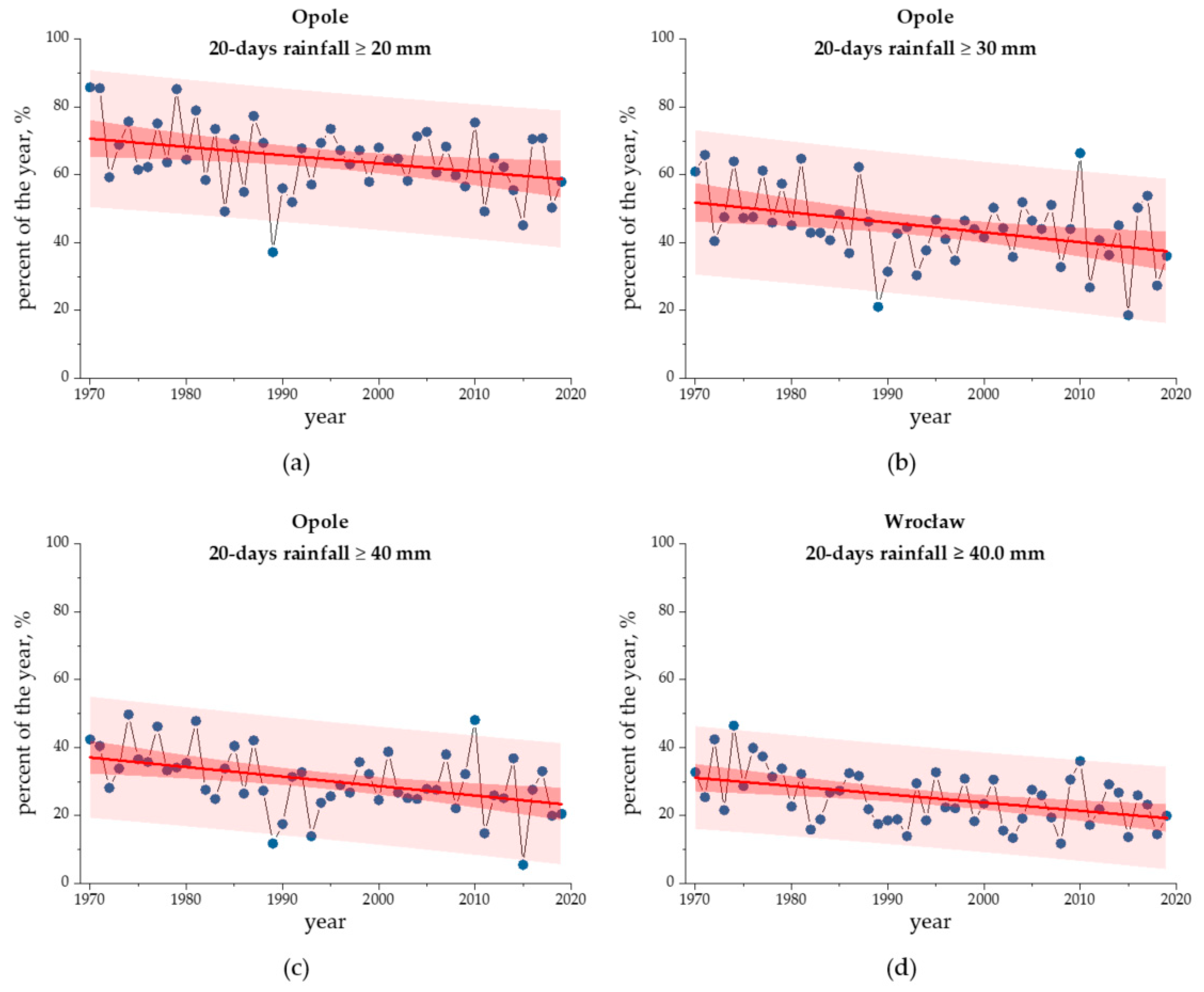
Opole	−156	−0.09	81%	−272	−0.26	98%	−296	−0.26	99%	−385	−0.27	99.9%
Poznań	120	0.07	68%	150	0.16	79%	161	0.17	82%	188	0.14	88%
Rzeszów	113	0.07	65%	51	0.05	32%	−14	−0.02	9%	−53	−0.04	34%
Suwałki	118	0.07	67%	169	0.14	84%	126	0.11	70%	122	0.09	69%
Szczecin	179	0.14	86%	153	0.13	80%	136	0.15	74%	121	0.12	68%
Toruń	147	0.11	78%	10	0.01	6%	23	0.03	15%	24	0.02	15%
Warsaw	136	0.10	74%	56	0.06	35%	86	0.07	52%	−6	0.00	3%
Wrocław	−37	−0.02	24%	−169	−0.11	84%	−194	−0.17	89%	−352	−0.23	99.7%
Zielona Góra	41	0.03	26%	109	0.09	63%	228	0.17	94%	120	0.11	68%

summarises these results, including the statistic S and the CLI. To increase the readability of the table, statistically significant changes ($CLI$ ≥ 95%), changes close to statistical significance ($CLI$ from 90 to 95%) and tendencies to change ($CLI$ from 75 to 90%) are highlighted blue (increasing) and yellow (decreasing).

In the analysed period, statistically significant decreasing trends for a 20-day cumulative rainfall higher than 20, 30 and 40 mm were found in Opole, and for cumulative rainfall over 40 mm in Wrocław. Additionally, upward trends close to statistical significance were detected Koszalin and Zielona Góra. Also, the assessment discovered tendencies to change (both signs) in other additional 15 cases. Figure 7 presents the plot of statistically significant trends for Opole and Wrocław, based on Equations (3)–(7), with the analysed precipitation 95% confidence limits for median marked as the narrow area in red, and the 95% prediction bounds for observations in pink.

Furthermore,

Table 5. Trend detection parameters for 20-day cumulative rainfall for the different class intervals under study, during the period 1970–2019.

City	Cumulative 20-Day Rainfall [0–10) mm			Cumulative 20-Day Rainfall [10–20) mm			Cumulative 20-Day Rainfall [20–30) mm			Cumulative 20-Day Rainfall [30–40) mm
	$\mathit{S}$	$\mathit{\beta }$(%)	$\mathit{C}\mathit{L}\mathit{I}$	$\mathit{S}$	$\mathit{\beta }$(%)	$\mathit{C}\mathit{L}\mathit{I}$	$\mathit{S}$	$\mathit{\beta }$(%)	$\mathit{C}\mathit{L}\mathit{I}$	$\mathit{S}$	$\mathit{\beta }$(%)	$\mathit{C}\mathit{L}\mathit{I}$
Białystok	−39	−0.04	25%	−104	−0.06	61%	−129	−0.06	72%	132	0.05	73%
Gdańsk	24	0.02	15%	100	0.07	59%	174	0.08	85%	−162	−0.07	82%
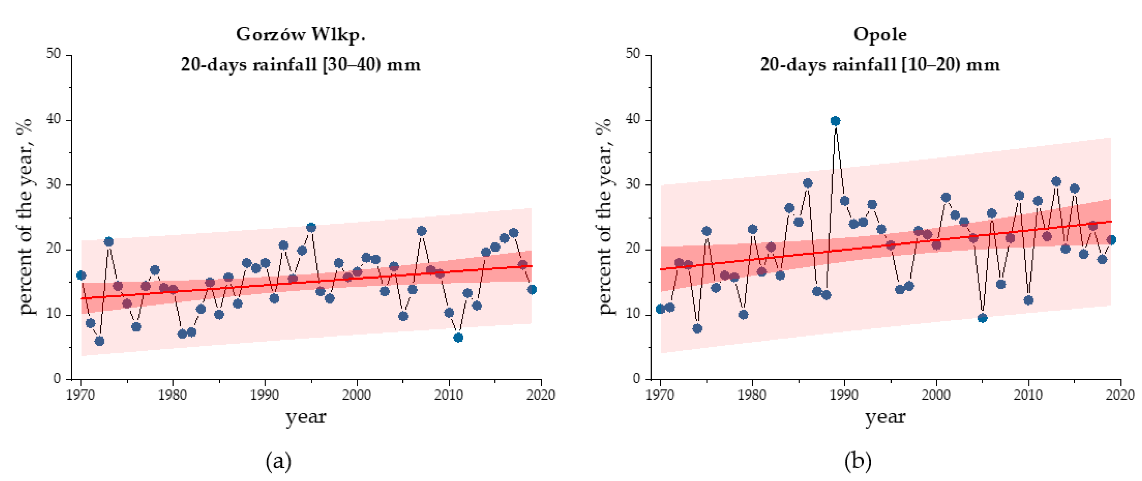
Gorzów Wlkp.	−124	−0.07	70%	−125	−0.08	70%	−16	0.00	10%	271	0.11	98%
Katowice	−2	0.00	1%	169	0.07	84%	163	0.07	82%	49	0.03	31%
Kielce	−95	−0.05	57%	126	0.07	70%	−51	−0.03	32%	−21	0.00	13%
Koszalin	−203	−0.10	91%	−23	−0.01	15%	89	0.03	54%	209	0.08	92%
Kraków	10	0.00	6%	30	0.02	19%	76	0.04	47%	−71	−0.03	44%
Lublin	−175	−0.11	85%	184	0.09	87%	−57	−0.02	36%	−111	−0.05	64%
Łódź	−15	−0.01	9%	−74	−0.03	46%	156	0.07	81%	42	0.02	27%
Olsztyn	−105	−0.05	62%	44	0.02	28%	94	0.05	56%	−43	−0.02	27%
Opole	156	0.09	81%	268	0.15	97%	97	0.06	58%	−25	−0.01	16%
Poznań	−120	−0.07	68%	−202	−0.12	91%	−55	−0.03	35%	51	0.03	32%
Rzeszów	−113	−0.07	65%	69	0.03	43%	57	0.02	36%	187	0.09	88%
Suwałki	−118	−0.07	67%	−114	−0.05	66%	43	0.02	27%	34	0.01	22%
Szczecin	−179	−0.14	86%	−61	−0.03	38%	52	0.02	33%	109	0.04	63%
Toruń	−147	−0.11	78%	130	0.07	72%	38	0.02	24%	−62	−0.02	39%
Warsaw	−136	−0.10	74%	36	0.02	23%	4	0.00	2%	204	0.06	91%
Wrocław	37	0.02	24%	162	0.10	82%	86	0.03	52%	159	0.08	81%
Zielona Góra	−41	−0.03	26%	−229	−0.11	94%	−116	−0.04	66%	210	0.09	92%

summarises the trend detection assessment results for the annual fraction with 20-day cumulative rainfalls for the intervals of [0–10) mm, [10–20) mm, [20–30) mm, and [30–40) mm. To increase the readability of the table, statistically significant changes ($CLI$ ≥ 95%), changes close to statistical significance ($CLI$ from 90 to 95%) and tendencies to change ($CLI$ from 75 to 90%) are highlighted blue (increasing) and yellow (decreasing).

There is evidence of statistically significant upward trends for Gorzów Wielkopolski ([30–40) mm) and Opole ([10–20) mm), and Figure 8 presents these results. Similarly, trends close to statistical significance were detected for Koszalin (downwards for [0–10) mm and upwards for [30–40) mm), Poznań (decreasing for [10–20) mm), Warsaw (increasing for [30–40) mm) and Zielona Góra (downwards for [10–20) mm and upwards for [30–40) mm). The results for Białystok, Kielce, Olsztyn and Suwałki suggest a stationary behaviour when considering these intervals of 20-day cumulative rainfall.

It is worth noting that for Poznań the amount of 20-day rainfall sums in the ranges [0–10) mm (CLI = 68%) and [10–20) mm (CLI = 91%) decreased, while there was no increase in the ranges [20–30) mm and [30–40) mm. However, let us observe (Table 4) that Poznań is the only city in which a clear upward trend in the 20-day rainfall sums exceeding 40 mm (CLI = 88%) was noted. It follows that in Poznań the occurrence frequency of very large 20-day rainfall sums exceeding 40 mm is increasing.

4. Discussion

From the results presented in the previous section, the observed frequency and behaviour of 20-day cumulative rainfall exceeding individual threshold values (≥10, ≥20, ≥30 and ≥40 mm), as well as class intervals ([0–10), [10–20), [20–30) and [30–40) mm), are similar in the 19 analysed locations, especially concerning their average and standard deviation with no clear outliers in any of these intervals. However, regions with smaller rainwater harvesting potential can be distinguished (e.g., Gdańsk and Poznań), as well as those with a higher rainwater harvesting potential (e.g., Katowice and Koszalin). The indicated areas (with higher and lower rainwater harvesting potential) are closely related to the climatological characteristics and topographic location of individual regions of Poland. The spatial diversity of annual rainfall in the analyzed multi-year period was shown in Figure 3. On the one hand, the proximity of the Baltic Sea in the north of the country and mountain ranges in the south, on the other hand the most common southwestern atmospheric circulation, causes the occurrence of higher rainfall magnitudes—both annual and interval cumulative values.

With respect to [42,43] the strongest decreasing trends were observed mainly in the south and west of Poland, especially 20-day cumulative rainfall exceeding 20, 30 and 40 mm. The weakest trends were mainly recorded in central, eastern and northeastern Poland, where most of the rainfall increasing trends were weak and poorly distributed spatially. Twenty-day cumulative rain over 40 mm occurred in densely populated regions with strong with a strong influence of socio-economic development, which corresponds to [43,44].

Except for Opole and Wrocław, all the regions, exhibit stationarity or an upward trend in their cumulative 20-day rainfall over 10 mm and 20 mm (see Table 4). This behaviour means that the design and overall performance of small and medium-sized RWH systems would not be affected by climate variability anytime soon, at least based on the results using the 1970–2019 time-series as a baseline. In Opole, the increase in the total fraction of the year with 20-day cumulative rainfall between 10 and 20 mm occurs at the expense of statistically significant decrements of periods with rainfall over 20 mm. It is also worth noticing the case of Gorzów Wielkopolski, whose statistically upward trend for 20-day cumulative rain for the interval [30–40) mm would represent a 1.1% average increment per decade, implying that the possibility for larger RWH systems in the region is increasing.

Statistically significant decreasing trends in the annual fraction of the year with 20-day cumulative rainfall over 20, 30 and 40 mm for Opole (changes at approximately −2.6% per decade) and above 40 mm for Wrocław (changes at −2.3% per decade) may have an impact on reducing the potential for rainwater use in single-family housing in these cities, especially in the case of higher water demand (larger tanks). However, environmental policies [58] and the research and development of water-efficient appliances [59,60] could help to mitigate the negative impact of these detected trends, and might even improve the overall performance of the existing RWH systems.

Based on the results in Table 3 and their corresponding behaviour summarised in Table 5, approximately 40% of 20-day cumulative precipitations occur in the interval between 10 and 30 mm. This percentage was found by averaging the means of the 20-day cumulative rainfall of the second and third class intervals in Table 2, and it also matches the precipitation behaviour described in Figure 4, with most of the stations presenting monthly averages below 50 mm between September and April. As stated by Semaan et al. [21], this knowledge is important because the adequate sizing of RWH systems is synonym to optimising their operation. Undersizing the system results in insufficient and unreliable water supply, while oversizing augments capital costs with minimum marginal benefits, as well as posing potential water quality risks.

The results in Table 2 show that 20-day cumulative rainfall events exceed 40 mm around 30% of the year. This situation provides the possibility of water management policies and projects focused on improving the quality and recharging groundwater resources. Groundwater aquifers are present in about 90% of the country [61], and they are a vital source of potable water for Poland. Still, they are currently endangered by the mining industry, fracking and other industrial activities [61,62,63,64].

Receptivity to RWH systems is usually positive for a wide range of everyday uses. However, costs related to their operation and maintenance, linked to the uncertainty regarding the rainfall regime are common hindrances to their extensive implementation [16]. Therefore, studies such as this one become useful water management tools, both for overcoming these barriers and for improving water resources management.

5. Conclusions

This paper assessed how long-term trends in precipitation in Poland might impact the design and operational conditions of RWH systems and resource availability. The study analysed the presence of trends in the rainfall time-series for 19 cities in Poland for years 1970–2019, from the perspective of design and operation of RWH systems. Therefore, there were analysed the 20-day cumulative rainfall periods along the year higher than the thresholds 10, 20, 30 and 40 mm, as well as the class intervals [0–10) mm, [10–20) mm, [20–30) mm and [30–40) mm. The results of the M–K test detected statistically significant (CLI ≥ 95%) or close to statistical significance (90% ≤ CLI < 95%) trends in 14 of the 152 datasets under analysis (9.2% of the total), and tendencies to change (75% ≤ CLI < 90%) in approximately 18% of the datasets, with less than half of them corresponding to downward trends. Most of the datasets exhibit stationary behaviour during the 50-year long period, and our findings suggest that the majority of the cities would not be negatively affected by changes in the rainfall regime, except for Wrocław and Opole. However, these changes in rainfall would represent a variation of less than 3% a decade, an impact that can be feasibly offset by policies and water-efficient devices.

The findings of this study are useful assets for integrated water management and sustainable planning in Poland, a European country with one of the lowest water availability index. By improving the understanding of hydrological variability, the assessments of trends and behaviour of hydrometeorological time-series help to reduce the uncertainty during the planning stages of RWH systems, which is a common obstacle to implementing these water storage technologies.

References

- Gutry-Korycka, M.; Sadurski, A.; Kundzewicz, Z.; Pociask-Karteczka, J.; Skrzypczyk, L.; Pociask-Karteczka, J. Zasoby wodne a ich wykorzystanie. Nauka 2014, 1, 77–98. [Google Scholar]
- Olichwer, T. Long-term variability of water resources in mountainous areas: Case Study—Kłodzko region (SW Poland). Carpathian J. Earth Environ. Sci. 2019, 14, 29–38. [Google Scholar] [CrossRef]
- Małecki, Z.J.; Gołębiak, P. Zasoby wodne Polski i świata. Zesz. Nauk. Inżynieria Lądowa Wodna Kształtowaniu Środowiska 2012, 7, 50–56. [Google Scholar]
- Kuczyński, W.; Zuchowicki, W. Ocena aktualnej sytuacji w zaopatrzeniu w wode{ogonek} w Polsce na tle sytuacji w świecie. Rocz. Ochr. Sr. 2011, 12, 419–465. [Google Scholar]
- Orlińska-Woźniak, P.; Wilk, P.; Gębala, J. Water availability in reference to water needs in Poland. Meteorol. Hydrol. Water Manag. 2014, 1, 45–50. [Google Scholar] [CrossRef][Green Version]
- Suchożebrski, J. Zasoby wodne Polski. In Zarządzanie Zasobami Wodnymi w Polsce; Global Compact Network Poland: Warsaw, Poland, 2018; pp. 92–96. [Google Scholar]
- Panasiuk, D.; Suduk, O.; Skrypchuk, P.; Miłaszewski, R. Comparison of the water footprint in Poland and Ukraine. Ekon. Środowisko 2018, 4, 112–123. [Google Scholar]
- Michalczyk, Z. Odpływ średni, zmienność w czasie i zróżnicowanie przestrzenne. In Hydrologia Polski; Jokiel, P., Marszelewski, W., Pociask-Karteczka, J., Eds.; Wydawnictwo Naukowe PWN SA: Warsaw, Poland, 2017; ISBN 978-83-01-19618-9. [Google Scholar]
- Hegerl, G.C.; Black, E.; Allan, R.P.; Ingram, W.J.; Polson, D.; Trenberth, K.E.; Chadwick, R.S.; Arkin, P.A.; Sarojini, B.B.; Becker, A.; et al. Challenges in Quantifying Changes in the Global Water Cycle. Bull. Am. Meteorol. Soc. 2015, 96, 1097–1115. [Google Scholar] [CrossRef]
- Falloon, P.; Betts, R. Climate impacts on European agriculture and water management in the context of adaptation and mitigation—The importance of an integrated approach. Sci. Total Environ. 2010, 408, 5667–5687. [Google Scholar] [CrossRef]
- Kundzewicz, Z.W.; Matczak, P. Climate change regional review: Poland. Wiley Interdiscip. Rev. Clim. Chang. 2012, 3, 297–311. [Google Scholar] [CrossRef]
- Lipińska, D. European Union Water Policy: Key Issues and Challenges. Comp. Econ. Res. Cent. East Eur. 2012, 15, 123–141. [Google Scholar] [CrossRef][Green Version]
- Kutyłowska, M. Forecasting failure rate of water pipes. Water Supply 2019, 19, 264–273. [Google Scholar] [CrossRef]
- Piasecki, A.; Jurasz, J.; Kaźmierczak, B. Forecasting Daily Water Consumption: A Case Study in Torun, Poland. Period. Polytech. Civ. Eng. 2018, 62, 818–824. [Google Scholar] [CrossRef]
- Dawidowicz, J.; Czapczuk, A.; Piekarski, J. The Application of Artificial Neural Networks in the Assessment of Pressure Losses in Water Pipes in the Design of Water Distribution Systems. Rocz. Ochr. Środowiska 2018, 20, 292–308. [Google Scholar]
- Ward, S.; Barr, S.; Memon, F.; Butler, D. Rainwater harvesting in the UK: Exploring water-user perceptions. Urban. Water J. 2013, 10, 112–126. [Google Scholar] [CrossRef]
- Steffen, J.; Jensen, M.; Pomeroy, C.A.; Burian, S.J. Water Supply and Stormwater Management Benefits of Residential Rainwater Harvesting in U.S. Cities. JAWRA J. Am. Water Resour. Assoc. 2013, 49, 810–824. [Google Scholar] [CrossRef]
- Torres, M.N.; Fontecha, J.E.; Zhu, Z.; Walteros, J.L.; Rodríguez, J.P. A participatory approach based on stochastic optimization for the spatial allocation of Sustainable Urban Drainage Systems for rainwater harvesting. Environ. Model. Softw. 2020, 123, 104532. [Google Scholar] [CrossRef]
- Deitch, M.J.; Feirer, S.T. Cumulative impacts of residential rainwater harvesting on stormwater discharge through a peri-urban drainage network. J. Environ. Manag. 2019, 243, 127–136. [Google Scholar] [CrossRef]
- Teston, A.; Teixeira, C.; Ghisi, E.; Cardoso, E. Impact of Rainwater Harvesting on the Drainage System: Case Study of a Condominium of Houses in Curitiba, Southern Brazil. Water 2018, 10, 1100. [Google Scholar] [CrossRef]
- Semaan, M.; Day, S.D.; Garvin, M.; Ramakrishnan, N.; Pearce, A. Optimal sizing of rainwater harvesting systems for domestic water usages: A systematic literature review. Resour. Conserv. Recycl. X 2020, 6, 100033. [Google Scholar] [CrossRef]
- Council of the European Union. Council Directive 98/83/EC of 3 November 1998 on the Quality of Water Intended for Human Consumption; Council of the European Union: Brussel, Belgium, 1998. [Google Scholar]
- European Parliament; Council of the European Union. Directive 2006/7/EC of the European Parliament and of the Council of 15 February 2006 Concerning the Management of Bathing Water Quality and Eepealing Directive 76/160/EEC; Council of the European Union: Brussel, Belgium, 2006. [Google Scholar]
- Jeong, G.Y.; Kim, J.Y.; Seo, J.; Kim, G.M.; Jin, H.C.; Chun, Y. Long-range transport of giant particles in Asian dust identified by physical, mineralogical, and meteorological analysis. Atmos. Chem. Phys. 2014, 14, 505–521. [Google Scholar] [CrossRef]
- Richon, C.; Dutay, J.-C.; Dulac, F.; Wang, R.; Balkanski, Y. Modeling the biogeochemical impact of atmospheric phosphate deposition from desert dust and combustion sources to the Mediterranean Sea. Biogeosciences 2018, 15, 2499–2524. [Google Scholar] [CrossRef]
- Orlović-Leko, P.; Vidović, K.; Ciglenečki, I.; Omanović, D.; Sikirić, M.D.; Šimunić, I. Physico-Chemical Characterization of an Urban Rainwater (Zagreb, Croatia). Atmos. Basel 2020, 11, 144. [Google Scholar] [CrossRef]
- Kieber, R.J.; Peake, B.; Willey, J.D.; Avery, G.B. Dissolved organic carbon and organic acids in coastal New Zealand rainwater. Atmos. Environ. 2002, 36, 3557–3563. [Google Scholar] [CrossRef]
- Zdeb, M.; Zamorska, J.; Papciak, D.; Słyś, D. The Quality of Rainwater Collected from Roofs and the Possibility of Its Economic Use. Resources 2020, 9, 12. [Google Scholar] [CrossRef]
- Kus, B.; Kandasamy, J.; Vigneswaran, S.; Shon, H.K. Analysis of first flush to improve the water quality in rainwater tanks. Water Sci. Technol. 2010, 61, 421–428. [Google Scholar] [CrossRef]
- Song, Y.; Du, X.; Ye, X. Analysis of Potential Risks Associated with Urban Stormwater Quality for Managed Aquifer Recharge. Int. J. Environ. Res. Public Health 2019, 16, 3121. [Google Scholar] [CrossRef]
- Willey, J.D.; Kieber, R.J.; Eyman, M.S.; Avery, G.B. Rainwater dissolved organic carbon: Concentrations and global flux. Glob. Biogeochem. Cycles 2000, 14, 139–148. [Google Scholar] [CrossRef]
- Helmreich, B.; Horn, H. Opportunities in rainwater harvesting. Desalination 2009, 248, 118–124. [Google Scholar] [CrossRef]
- Kaushik, R.; Balasubramanian, R. Assessment of bacterial pathogens in fresh rainwater and airborne particulate matter using Real-Time PCR. Atmos. Environ. 2012, 46, 131–139. [Google Scholar] [CrossRef]
- Leong, J.Y.C.; Oh, K.S.; Poh, P.E.; Chong, M.N. Prospects of hybrid rainwater-greywater decentralised system for water recycling and reuse: A review. J. Clean. Prod. 2017, 142, 3014–3027. [Google Scholar] [CrossRef]
- Al-Khatib, I.; Arafeh, G.; Al-Qutob, M.; Jodeh, S.; Hasan, A.; Jodeh, D.; van der Valk, M. Health Risk Associated with Some Trace and Some Heavy Metals Content of Harvested Rainwater in Yatta Area, Palestine. Water 2019, 11, 238. [Google Scholar] [CrossRef]
- Huston, R.; Chan, Y.C.; Chapman, H.; Gardner, T.; Shaw, G. Source apportionment of heavy metals and ionic contaminants in rainwater tanks in a subtropical urban area in Australia. Water Res. 2012, 46, 1121–1132. [Google Scholar] [CrossRef] [PubMed]
- Mendez, C.B.; Klenzendorf, J.B.; Afshar, B.R.; Simmons, M.T.; Barrett, M.E.; Kinney, K.A.; Kirisits, M.J. The effect of roofing material on the quality of harvested rainwater. Water Res. 2011, 45, 2049–2059. [Google Scholar] [CrossRef] [PubMed]
- Gikas, G.D.; Tsihrintzis, V.A. Effect of first-flush device, roofing material, and antecedent dry days on water quality of harvested rainwater. Environ. Sci. Pollut. Res. 2017, 24, 21997–22006. [Google Scholar] [CrossRef] [PubMed]
- Sneyers, R. On the Statistical Analysis of Series of Observations. WMO Technical Note No.143; World Meteorological Organization: Geneva, Switzerland, 1990. [Google Scholar]
- Coombes, P.J.; Barry, M.E. The effect of selection of time steps and average assumptions on the continuous simulation of rainwater harvesting strategies. Water Sci. Technol. 2007, 55, 125–133. [Google Scholar] [CrossRef] [PubMed]
- IMGW Polish Institute of Meteorology and Water Management—National Research Institute (IMGW). Available online: https://www.imgw.pl/instytut/imgw-pib (accessed on 2 January 2020).
- Pińskwar, I.; Choryński, A.; Graczyk, D.; Kundzewicz, Z.W. Observed changes in extreme precipitation in Poland: 1991–2015 versus 1961–1990. Theor. Appl. Climatol. 2018, 135, 773–787. [Google Scholar] [CrossRef]
- Lupikasza, E. Spatial and temporal variability of extreme precipitation in Poland in the period 1951–2006. Int. J. Climatol. 2010, 30, 991–1007. [Google Scholar] [CrossRef]
- Kaźmierczak, B.; Wdowikowski, M.; Gwoździej-Mazur, J. Trends in daily changes of precipitation on the example of Wrocław. Ekon. Sr. 2019, 1, 142–151. [Google Scholar]
- Urban, G.; Richterová, D.; Kliegrová, S.; Zusková, I. Durability of snow cover and its long-term variability in the Western Sudetes Mountains. Theor. Appl. Climatol. 2019, 137, 2681–2695. [Google Scholar] [CrossRef]
- Struk-Sokołowska, J.; Gwoździej-Mazur, J.; Jadwiszczak, P.; Butarewicz, A.; Ofman, P.; Wdowikowski, M.; Kaźmierczak, B. The Quality of Stored Rainwater for Washing Purposes. Water 2020, 12, 252. [Google Scholar] [CrossRef]
- Ndehedehe, C.E.; Ferreira, V.G. Assessing land water storage dynamics over South America. J. Hydrol. 2020, 580, 124339. [Google Scholar] [CrossRef]
- Sharma, S.; Mujumdar, P.P. On the relationship of daily rainfall extremes and local mean temperature. J. Hydrol. 2019, 572, 179–191. [Google Scholar] [CrossRef]
- Ali, R.; Ismael, A.; Heryansyah, A.; Nawaz, N. Long Term Historic Changes in the Flow of Lesser Zab River, Iraq. Hydrology 2019, 6, 22. [Google Scholar] [CrossRef]
- Langat, P.; Kumar, L.; Koech, R. Temporal Variability and Trends of Rainfall and Streamflow in Tana River Basin, Kenya. Sustainability 2017, 9, 1963. [Google Scholar] [CrossRef]
- Arrieta-Castro, M.; Donado-Rodríguez, A.; Acuña, G.J.; Canales, F.A.; Teegavarapu, R.S.V.; Kaźmierczak, B. Analysis of Streamflow Variability and Trends in the Meta River, Colombia. Water 2020, 12, 1451. [Google Scholar] [CrossRef]
- Jaiswal, R.K.; Lohani, A.K.; Tiwari, H.L. Statistical Analysis for Change Detection and Trend Assessment in Climatological Parameters. Environ. Process. 2015, 2, 729–749. [Google Scholar] [CrossRef]
- Wijngaard, J.B.; Klein Tank, A.M.G.; Können, G.P. Homogeneity of 20th century European daily temperature and precipitation series. Int. J. Climatol. 2003, 23, 679–692. [Google Scholar] [CrossRef]
- Ledvinka, O.; Lamacova, A. Detection of field significant long-term monotonic trends in spring yields. Stoch. Environ. Res. Risk Assess. 2015, 29, 1463–1484. [Google Scholar] [CrossRef]
- Yue, S.; Pilon, P.; Phinney, B.; Cavadias, G. The influence of autocorrelation on the ability to detect trend in hydrological series. Hydrol. Process. 2002, 16, 1807–1829. [Google Scholar] [CrossRef]
- Onyutha, C. Statistical Uncertainty in Hydrometeorological Trend Analyses. Adv. Meteorol. 2016, 2016, 8701617. [Google Scholar] [CrossRef]
- Wagesho, N.; Goel, N.K.; Jain, M.K. Investigation of non-stationarity in hydro-climatic variables at Rift Valley lakes basin of Ethiopia. J. Hydrol. 2012, 444–445, 113–133. [Google Scholar] [CrossRef]
- Makki, A.A.; Stewart, R.A.; Panuwatwanich, K.; Beal, C. Revealing the determinants of shower water end use consumption: Enabling better targeted urban water conservation strategies. J. Clean. Prod. 2013, 60, 129–146. [Google Scholar] [CrossRef]
- Lee, M.; Tansel, B.; Balbin, M. Influence of residential water use efficiency measures on household water demand: A four year longitudinal study. Resour. Conserv. Recycl. 2011, 56, 1–6. [Google Scholar] [CrossRef]
- Lee, M.; Tansel, B. Water conservation quantities vs customer opinion and satisfaction with water efficient appliances in Miami, Florida. J. Environ. Manag. 2013, 128, 683–689. [Google Scholar] [CrossRef] [PubMed]
- Polish Geological Institute Groundwater Resources in Poland. Available online: https://www.pgi.gov.pl/en/phs/tasks/8862-groundwater-resources-in-poland.html (accessed on 6 June 2020).
- Witkowski, A.J.; Kowalczyk, A.; Rubin, H.; Rubin, K. Groundwater quality and migration of pollutants in the multi-aquifer system of the former chemical works “Tarnowskie Góry” area. Polish Geol. Inst. Spec. Pap. 2008, 24, 123–130. [Google Scholar]
- Montcoudiol, N.; Isherwood, C.; Gunning, A.; Kelly, T.; Younger, P.L. Shale gas impacts on groundwater resources: Understanding the behavior of a shallow aquifer around a fracking site in Poland. Energy Procedia 2017, 125, 106–115. [Google Scholar] [CrossRef]
- Jakóbczyk-Karpierz, S.; Ślósarczyk, K.; Sitek, S. Tracing multiple sources of groundwater pollution in a complex carbonate aquifer (Tarnowskie Góry, southern Poland) using hydrogeochemical tracers, TCE, PCE, SF6 and CFCs. Appl. Geochem. 2020, 118. [Google Scholar] [CrossRef]