Application of GWO-ELM Model to Prediction of Caojiatuo Landslide Displacement in the Three Gorge Reservoir Area

Abstract

In order to establish an effective early warning system for landslide disasters, accurate landslide displacement prediction is the core. In this paper, a typical step-wise-characterized landslide (Caojiatuo landslide) in the Three Gorges Reservoir (TGR) area is selected, and a displacement prediction model of Extreme Learning Machine with Gray Wolf Optimization (GWO-ELM model) is proposed. By analyzing the monitoring data of landslide displacement, the time series of landslide displacement is decomposed into trend displacement and periodic displacement by using the moving average method. First, the trend displacement is fitted by the cubic polynomial with a robust weighted least square method. Then, combining with the internal evolution rule and the external influencing factors, it is concluded that the main external trigger factors of the periodic displacement are the changes of precipitation and water level in the reservoir area. Gray relational degree (GRG) analysis method is used to screen out the main influencing factors of landslide periodic displacement. With these factors as input items, the GWO-ELM model is used to predict the periodic displacement of the landslide. The outcomes are compared with the nonoptimized ELM model. The results show that, combined with the advantages of the GWO algorithm, such as few adjusting parameters and strong global search ability, the GWO-ELM model can effectively learn the change characteristics of data and has a better and relatively stable prediction accuracy.

1. Introduction

Landslide is one of the worst geological disasters in many areas of the world, with the characteristics of wide distribution, strong paroxysm, high frequency and great harmfulness. Landslide disaster can not only cause a large number of casualties and property losses, but also bring huge damage to resources, environment and ecology [1]. The Three Gorges Reservoir area in China is prone to landslides due to the special complicated natural geological conditions and heavy rainfall every year [2,3]. Landslide prediction is an important subject in the study of landslide disaster, an effective way to prevent and control landslide disaster, and can reduce the loss caused by landslide disaster, which has important theoretical and practical significance [4]. However, the landslide is a complex multidimensional nonlinear dynamic system [5], and its displacement is the result of the interaction of internal geological conditions and external factors. The formation of landslide displacement is characterized by the complexity of its own geological conditions, the diversity and randomness of external induced factors, so it is highly uncertain. Researchers around the world have yet to fully explore and reveal the underlying mechanism. It is generally believed that the internal factors include gravity stress, pore fluid pressure, stratigraphic lithology and other physical properties of landslides, while the external trigger factors include earthquake, fluctuation of reservoir water level and human activities, etc. External factors break the original stress balance and eventually lead to landslides [6,7]. The uncertainty leads to the unclear identification of the evolution of landslide system, which has a great impact on the accurate prediction of landslide.

Landslide displacement prediction has been a hot topic in geological disaster research at home and abroad for a long time. With the rapid development of artificial intelligence and machine learning, a large number of data mining methods and nonlinear intelligent integrated systems have been well applied in landslide displacement prediction. Compared with the traditional physical prediction model [8] based on formula or professional software [9], the landslide prediction model combined with machine method has a simple principle, controllable precision and strong adaptability [10]. The representative ones are Neural Network Model [11], Gray Model [12], Verhulst Mode [13], and Support Vector Machine Model (SVM) [14], etc. Machine learning has been explored as a powerful method to predict displacement and has achieved good results. Du [15] decomposed the cumulative displacement into trend component and periodic component, and used the back propagation neural network (BPNN) to predict the periodic displacement. Polykretis [16] and Lian [17] applied artificial neural network (ANN) to landslide displacement prediction. Pradhan [18] conducted a comparative study using support vector machines (SVM) and neuro-fuzzy models to test their performance in predicting displacement. Chousianitis [19] used the Newmark model to construct a mapping between geological parameters and earthquake-induced landslides. Li [20] employed continuous wavelet analysis to decompose the time-series precipitation, reservoir water level, and displacement into seasonal and residual components, and utilized the exponentially weighted moving average (EWMA) control chart to derive the boundaries as alarm conditions of seasonal faster displacement. Although these intelligent algorithms have achieved some results, they also have some limitations. For example, when the neural network learning algorithm (BP algorithm) is initialized, the network training parameters in the algorithm must be set, which usually leads to the occurrence of the local optimal solution. SVM has a better prediction effect than the neural network model, but the model itself has some defects, such as having difficulty in parameter selection. Extreme Learning Machine (ELM) [21] is a newly proposed algorithm in recent years which is based on Single-hidden Layer Feedforward Neural Network (SLFNs). ELM solved the problems of determining the number of hidden layers neural network. Compared with the traditional prediction models such as BP neural network and SVM, ELM has the advantages of fast learning speed, good generalization ability and producing the only optimal solution [22]. The classification accuracy of ELM can be greatly improved by setting appropriate model parameters [23]. In traditional methods, these parameters are mainly set through a grid search method, gradient descent algorithm and meta-heuristic search algorithm, such as Particle Swarm Optimization (PSO) and Genetic Algorithm (GA) [24]. Gray Wolf Optimizer (GWO) [25], as a new meta-heuristic algorithm that imitated the hunting behavior of wolves, has the advantages of having a simple principle, less adjustment parameters, strong global search ability, etc. It has been proven to have significant advantages in studying combinatorial optimization problems, and has been widely used in various fields [26]. In the landslide prediction field, Guo proposed a model based on wavelet analysis (WA) and BPNN optimized by the GWO algorithm (the GWO-BP model) and obtained good results. Jaafari [26] utilized the GWO algorithm to obtain a reliable estimate of landslide susceptibility. In this paper, a typical step-wise-characterized landslide called Caojiatuo landslide in the TGR area is taken as an example. Based on the time series analysis principle, the displacement is decomposed into two components: the trend displacement and periodic displacement [27]. The trend displacement is extracted by using the moving average method, and predicted by using the cubic polynomial function of the robust weighted least-square method. In this paper, the GWO is innovatively introduced into the ELM, and a landslide displacement prediction model based on GWO-ELM is proposed to predict the periodic displacement. Root-mean-square error (RMSE) and mean absolute percent error (MAPE) are applied as evaluation criteria to analyze the predicted results. This new model helps to build a more accurate landslide warning system.

2. The Proposed Landslide Displacement Prediction Model

2.1. Time Series Model

Landslide displacement is a nonstationary time series varying with time [5]. The study shows that the accumulative displacement of the landslide is caused by the interaction of the internal geological conditions (lithology, geological structure, landform, etc.), external environmental factors (precipitation, reservoir water level, etc.) and other random factors (uncertainty) [28]. The displacement of the landslide under the control of its own internal basic geological conditions is expressed as an approximately monotone increasing function varying with time, that is, the trend displacement. The displacement under the influence of external environmental factors is shown as an approximately periodic function which changes with seasonal rainfall and reservoir water level, namely the periodic displacement. Based on the above features, the time series decomposition theory is adopted to decompose the accumulative displacement of the landslide:

$$X\left(t\right)=\alpha \left(t\right)+\beta \left(t\right)+\gamma \left(t\right)$$

(1)

where $X\left(t\right)$ represents the monitored displacement; $\alpha \left(t\right)$ is the trend displacement; $\beta \left(t\right)$ is the periodic displacement; $\gamma \left(t\right)$ is the random displacement.

The random displacement is mainly caused by the random influencing factors (wind load, vehicle load and vibration load, etc.). Due to the limitation of the current monitoring technology, it is difficult to obtain the data of such factors, and the influence of them is relatively small. Generally, it is not considered in the research [29]. Therefore, Equation (1) can be simplified as follows:

$$X\left(t\right)=\alpha \left(t\right)+\beta \left(t\right)$$

(2)

Generally speaking, the trend displacement can be extracted by the moving average method, which can smooth the short-term fluctuation of time series and reflect the long-term trend. The specific calculation method is to assume that the monitoring value of landslide displacement at time $t$ is $s\left(t\right)$, and the trend displacement at time $t$ is $\beta \left(t\right)$. The calculation formula is as follows:

$$\beta \left(t\right)=\frac{s\left(t\right)+s\left(t-1\right)+\cdots +s\left(t-k+1\right)}{n}$$

(3)

where $t=k,k+1,\dots ,n$; $s\left(t-n+1\right)$ is the monitoring value of landslide displacement at time $t-n+1$; $n$ is the moving cycle.

Based on the time series decomposition theory, after the extraction of the trend displacement is completed, the periodic displacement $\alpha \left(t\right)$ is obtained by removing the trend displacement $\beta \left(t\right)$ from the accumulative displacement $X\left(t\right)$.

2.2. Extreme Learning Machine Model

ELM is a training method based on the Single-hidden Layer Feedforward Neural Network (SLFNs) [29]. The output weight of the network can be obtained by one-step calculation and analysis. In this process, the only optimal solution can be obtained and the learning speed is very high just by setting the threshold value of the neurons in the hidden layer. For N arbitrary and different samples $\left(x_i,y_i\right)$, where $x_i={\left[x_{i1},x_{i2},\dots ,x_{in}\right]}^T\in R^n$, $y_i={\left[y_{i1},y_{i2},\dots ,y_{im}\right]}^T\in R^m$, and there are L neuron nodes in the hidden layer. Then the output of the standard feedforward neural network, the excitation function of which is $g\left(x\right)$ can be expressed as:

$$f_L\left(x\right)={\displaystyle \sum _{i=1}^L{\beta }_{i}g\left(a_i\times x_i+b_i\right),x_i\in R^n},a\in R^n,{\beta }_i\in R^m$$

(4)

where $a_i={\left[a_{i1},a_{i2},\dots ,a_{in}\right]}^T$ is the input weight from the input layer to the nodal point of the $\mathrm{ith}$ hidden layer; $b_i$ is the threshold value of the $\mathrm{ith}$ neuron in the hidden layer; ${\beta }_i={\left[{\beta }_{i1},{\beta }_{i2},\dots ,{\beta }_{im}\right]}^T$ is the output weight connecting the $\mathrm{ith}$ node in the hidden layer; $a_i\times x_i$ is the inner product of vector $a_i$ and $x_i$; the excitation function $g\left(x\right)$ can be selected as “Sigmoid”, “RBF”, or “Sine”, etc.

If the standard feedforward neural network with L hidden layer neurons and excitation function $g\left(x\right)$ can approach these N samples with zero error, then there exist $a_i,b_i,c_i$ making the following equation true:

$$f_L\left(x\right)={\displaystyle \sum _{i=1}^L{\beta }_{i}g\left(a_i\times x_i+b_i\right)=y_i,i=1,2,\dots ,L}$$

(5)

Equation (5) can be simplified to:

$$H\beta =Y$$

(6)

where $H$ is the output matrix of the neural network. In ELM, the output weight and threshold are randomly given, and the hidden layer matrix $H$ namely becomes a definite matrix, which makes the training of feedforward neural network transform to a problem of finding the least square solution of the output weight matrix; the output weight matrix $\beta$ is:

$$\hat{\beta }=H^{+}Y$$

(7)

where $H^{+}$ represents the Moore-Penrose generalized inverse matrix of the hidden layer output matrix $H$, which can be obtained analytically by orthogonal projection or singular decomposition method, etc.

2.3. Gray Wolf Optimization

Gray Wolf Optimization (GWO) algorithm is a new swarm intelligent optimization algorithm proposed by MIRJALILI [25]. GWO simulates the process of the gray wolf hunting behavior such as wolf tracking, encircling, chasing, and attacking prey, so as to achieve the goal of optimization. GWO has the advantages of having a simple principle, few adjustment parameters, strong global search ability and so forth.

The optimization process of GWO is as follows: a group of gray wolves is randomly generated in the search space. According to the fitness level, the wolves numbered $\alpha ,\beta ,\delta$ in the gray wolf group evaluate and locate the position of the prey. The rest of the individuals take this as the standard, and calculate the distance between themselves and the prey to complete the prey capture and realize the optimization process [25].

Definition 1.

Social Hierarchy. The GWO model has a strict social class, which can be divided into$\alpha ,\beta ,\delta ,\omega$wolves on the basis of the social class. The social class in the algorithm is reflected in the fitness level.

Definition 2.

Encircling Prey. In the process of wolf hunting, they need to s encircle the prey and determine the location of the prey. The mathematical equations of encirclement behavior are as follows:

$$D=\left|C\times X_p\left(w\right)-X\left(w\right)\right|$$

(8)

$$X\left(w+1\right)=X_p\left(w\right)-\mu \times D$$

(9)

$$C=2\times r_1$$

(10)

$$\mu =2a\times r_2-a$$

(11)

where$w$is the current iteration number;$X_p\left(w\right)$is the position vector of the prey in generation$w$; $X\left(w\right)$is the position vector of individual gray wolf in generation$w$; $X\left(w+1\right)$is the position vector of individual gray wolf in generation$w+1$; $C$is coefficient vector;$r_1,r_2$belong to random vector, with the value range of [0, 1];$\mu$is a vector of convergence; the value of$a$declines linearly from 2 to 0 during the iteration.

Definition 3.

Hunting. The hunting process of wolves on prey is represented by the constant replacement of hunting location information. Specifically, in the iterative process, the algorithm saves the current locations of the best three wolves ($\alpha ,\beta ,\delta$), and updates the location of wolves in other search units ($\omega$) according to their information to obtain the optimal solution. Hunting behavior can be expressed as:

$$D_k=\left|C_i\times X_k\left(w\right)-X\left(w\right)\right|$$

(12)

$$X_i=X_k-{\mu }_i\times D_k$$

(13)

$$X_p\left(w+1\right)=\frac{X_1+X_2+X_3}{3}$$

(14)

where$k=\alpha ,\beta ,\gamma$; $i=1,2,3$; $X_p\left(w+1\right)$is the position vector of the prey in$w+1$generation.

2.4. Proposed Prediction Model Based on GWO-ELM

In this paper, based on the principle of time series, the accumulative displacement is decomposed into the trend and periodic displacement. For trend displacement, the robust weighted least squares cubic polynomial fitting projections is adopted. For periodic displacement, the GWO is introduced to the ELM model for training. The framework system of the proposed extreme learning machine model, namely GWO-ELM model, is shown in Figure 1.

3. Caojiatuo Landslide

3.1. Geologic Aspects

The Caojiatuo landslide [30] is in the TGR area of China. After the construction of the Three Gorges Dam, the hydrogeological conditions in this region has been dramatically changed and the TGR area has become a world-famous landslide-prone area. The Caojiatuo landslide, as one of the typical landslides, locates on the left bank of the Yangtze river, Wushan county, Hubei province (Figure 2). The plane shape of the landslide is close to a square approximately 600 m long and 500 m wide. The landslide occupies a mass with an area approximately 30 × 10⁴ m² and a volume approximately 1500 × 10⁴ m³ (Figure 3). The sliding surface was the interface between the loose accreted body and the underlying bedrock, with the length of approximately 600 m, the width of approximately 500 m, dip angle of 30°, and dip direction of 150° (Figure 4). The thickness of the contact zone was approximately 2 m, mainly comprising clay with a small amount of debris.

The landslide body is composed of colluvial and residual silty clay, which was yellow-brown and easily softened by water [2]. The material also contains approximately 35% rubble, which reduces from the surface to the bottom of the landslide mass, and consists of gray-green silty siltstone of size 5–10 cm. The bedrock mainly consisted of silty siltstone, gray-green marlite, and a small amount of magenta mudstone of the Badong Formation in the Triassic.

3.2. Monitoring Data Analysis

The water level of the TGR reached 135 m in 2003, and the Caojiatuo landslide was first deformed and tensile cracks appeared along the trailing edge. With the development of the landslide, the cracks increased year by year. In order to observe the surface deformation of the landslide and avoid catastrophic geological disasters, since 2007, the landslide was divided into two regions: zone A and zone B and nine GPS sensors (Figure 3) were installed to monitor the stability of the landslide per month, especially during the rainy season. Figure 5 shows the relationship between the monthly displacement of the 9 GPS observation points of Caojiatuo landslide and the reservoir water level and precipitation during 2007–2013. It can be seen that the displacement of block A (GPS-2, GPS-3, GPS-5, GPS-6) is a typical step-wise evolution process. The displacement of the landslide surface increased rapidly between May and July every year, and gradually approached a stable state in the following period. The displacement of block B (GPS-1, GPS-4, GPS-7, GPS-8, GPS-9) shows a different variation feature. The deformation of the monitoring points in block B was relatively small, and the fluctuation with the changes of the reservoir water level and precipitation was not obvious. Therefore, the deformation of the landslide mass of block B is defined as the trail-type deformation.

The accumulative displacement in block A was obviously affected by seasonal precipitation and reservoir water level, which is conducive to the study of factors affecting landslide deformation. The displacement values monitored by the GPS-6 and GPS-3 observation points in block A are relatively large. The monitoring data are representative and can effectively reflect the movement process of the whole landslide. Therefore, the data of GPS-6 and GPS-3 are selected for analysis in this paper. According to the curves of the monitored accumulative displacement, monthly precipitation and reservoir water level in Figure 5, the data can be divided into three stages:

(1) Stage 1 (7 January–9 May): The displacement growth was slow in this stage. According to the curve of reservoir water level, the reservoir began to fill water every year in September. Around January 2009, the maximum water level of the reservoir reached 175 m for the first time. With the increase of the reservoir water level, the displacement of the monitoring points in the current month did not change significantly, indicating that the influence of the rising reservoir water level on the displacement was weak. The water level of the reservoir reached the lowest value around May each year, and the displacement of the corresponding monitoring point increased to a certain extent after a month. The reason for the phenomenon was that the change of the water level inside the landslide lagged behind the water level. According to the precipitation curve, when seasonal heavy rainfall occurred in the landslide area (mainly from May to September every year), the landslide displacement continued to increase, which reflected the correlation between landslide displacement and rainfall. Therefore, in Stage 1, the displacement of monitoring points was mainly caused by rainfall, and the influence of reservoir water level was small.

(2) Stage 2 (9 May–12 January): The displacement increases sharply at the early time, while increased slowly in the subsequent period. The water level of the reservoir fluctuated between 145 m and 175 m. The landslide displacement corresponding to the peak water level of the reservoir remained relatively stable, which proved once again that the rising water level of the reservoir had a weak effect on the landslide displacement. Around May 2009, the area of the landslide was subjected to continuous heavy rainfall, and the water level of the reservoir reached the lowest value. The largest step-wise deformation in the landslide occurred, which could be considered as a result of the combined effect of reservoir water decline and high precipitation.

(3) Stage 3 (12 January–13 December): In this stage, displacement increased rapidly. The reservoir water level had the same fluctuation rule, but the seasonal rainfall generally intensified. When the water level of the reservoir reached the peak point, the displacement of the monitoring point did not change. However, under the combined effect of the peak precipitation and the lowest reservoir water level in May each year, the landslide displacement increased rapidly and the step-wise characteristics were strengthened.

4. Case Study

4.1. Prediction of Trend Displacement

According to the above discussion, the displacements of observation points GPS-6 and GPS-3 are selected as the study object. The trend displacement of the Caojiatuo landslide is extracted by using the moving average method (Equations (3) and (15)). The data from January 2008 to January 2013 are used as the training set to fit the equation, and the data from January 2013 to December 2013 are used to verify the accuracy of the fitting equation. The reservoir water level scheduling and GPS data in the TGR area all take a period of one month, that is, the movement period is set as $n=12$, which represents the 12 months of each year. Based on the time series addition principle, the trend displacement is removed from the monitoring accumulative displacement of the landslide to obtain the periodic displacement. The extraction results of the trend and period displacement of the observation points GPS-6 and GPS-3 are shown in Figure 6 and Figure 7, respectively.

The trend displacement is controlled by the geological conditions of the landslide and represents the main trend of landslide deformation. The trend displacement of GPS-6 and GPS-3 data are divided into four and three parts respectively, and the cubic polynomial based on the robust weighted least square method is used to fit the trend displacement on the time axis (Equation (15)). The calculated results of each coefficient of the fitting function are shown in

Table 1. Fitted results of the measured trend displacement.

Landslides	Monitoring Points	Period	a	b	c	d	R2
Caojiatuo Landslide	GPS-6	January 2008 to June 2009	0.019	−0.569	14.31	52.0	0.9987
		July 2009 to July 2010	−0.0794	5.665	−109.61	801.7	0.9998
		August 2010 to July 2012	0.0077	−0.886	38.65	−94.1	0.9982
		August 2012 to December 2013	−0.0238	4.132	−218.30	4090.7	0.9998
	GPS-3	January 2008 to June 2009	0.0152	−0.6089	13.317	51.855	0.9993
		July 2009 to July 2010	−0.0653	4.7216	−92.024	691.59	0.9996
		August 2010 to July 2013	−0.0025	0.6822	−40.139	1113	0.9949

. The fitting results are shown in Figure 8 and Figure 9. The trend displacement of the fitting equations is close to the measured value.

$$f\left(t\right)=a{t}^3+b{t}^2+ct+d$$

(15)

where $f\left(t\right)$ means the predictive values of the trend displacement at the time $t$; and $a,b,c,d$ are the coefficients, where $a$ cannot be equal to zero.

4.2. Prediction of Periodic Displacement

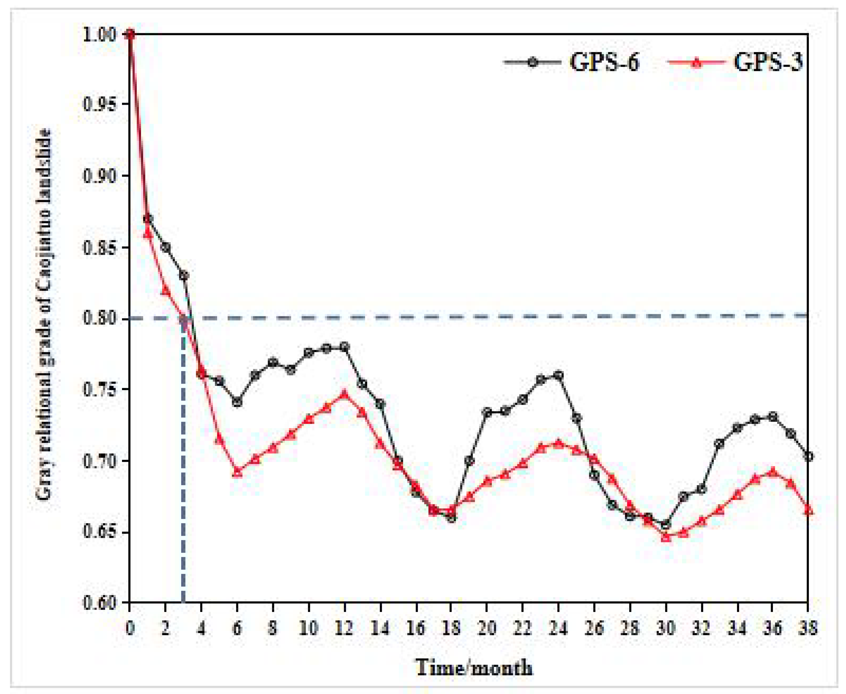
4.2.1. The External Influencing Factors

The prediction of periodic displacement is the key of landslide displacement prediction. In this model, the factors affecting the periodic displacement are taken as the input sequence and the periodic displacement as the output sequence. The selection of influencing factors directly affects the accuracy of model training. According to the above data analysis, the reservoir water level and precipitation are the two main factors affecting the periodic displacement.

Precipitation is one of the main external triggers of landslide deformation in the TGR area. On the one hand, the saturated soil is formed by water infiltration into the landslide, which increases the bulk density of the soil and reduces the stability of the landslide. On the other hand, the rain will induce the chemical reaction with the substance in the landslide, resulting in argillization and softening, which will further induce the occurrence of the landslide. Figure 10 shows the relationship between the periodic displacement of GPS-6 and GPS-3 and precipitation in the last one or two months. The precipitation in the last one or two months has a certain influence on the periodic displacement of the observation point. Both of them show fluctuation change, and the peak of periodic displacement generally lags behind the peak of precipitation. Therefore, the one-month and two-month cumulative antecedent rainfall are selected as the influencing factors of precipitation on the periodic displacement.

The periodic fluctuation of reservoir water level is another major factor leading to the step-wise deformation of the landslide. The change of reservoir water level will affect the distribution of groundwater dynamic field and the seepage field inside the landslide mass, which induce the deformation and damage of the landslide [31]. Figure 11 shows the relationship between the periodic fluctuation of the reservoir water level and the periodic displacement at the observation points GPS-6 and GPS-3. It can be clearly seen that the periodic fluctuation of water level has a certain correlation with the periodic displacement. In particular, when the water level drops sharply, the landslide deformation will be seriously affected. The effect of reservoir water level is usually a slow process, and there will be a so-called “hysteresis effect”. Therefore, reservoir level change in one-month and two-month period as well as the average elevation of reservoir level in the current month are selected as the influencing factors of reservoir water level on periodic displacement.

The same landslide affected by the same external triggers (precipitation, reservoir water level, etc.) may show completely different evolution characteristics in different stages. In the initial stable state, the landslide may remain stable even under the action of a strong external force. On the contrary, if the landslide is unstable at the beginning, or even in a highly unstable state, a relatively weak external force will eventually lead to great damage [32]. Therefore, this paper proposes to take the evolution state as a supplement to the factors of precipitation and reservoir water level to characterize the influence of other periodic factors on the landslide displacement. The landslide displacements over the past one, two and three months are selected respectively to represent the current evolution state of the landslide [33] as another three influencing factors.

Based on the above analysis, eight influencing factors related to periodic displacement are obtained. The correlation between periodic displacement and external triggering factors is analyzed based on the gray relational grade (GRG) theory [34,35,36,37,38,39,40,41,42,43,44,45,46,47]. According to the GRG theory, when the discrimination coefficient is 0.5, if the relational degree value corresponding to the influence factor is greater than or equal to 0.8, it means that the two are closely related.

Table 2. The gray relational grade (GRG) of input items between inducing factors and periodic displacement in the Caojiatuo landslide.

Input Item	GPS-6		GRG	GPS-3		GRG
Precipitation	Input 1	The one-month cumulative antecedent rainfall	0.83	Input 1	The one-month cumulative antecedent rainfall	0.82
	Input 2	The two-month cumulative antecedent rainfall	0.81	Input 2	two-month cumulative antecedent rainfall	0.80
Reservoir level	Input 3	Reservoir level change in one-month period	0.88	Input 3	Reservoir level change in one-month period	0.87
	Input 4	Reservoir level change in two-month period	0.86	Input 4	Reservoir level change in two-month period	0.84
	Input 5	The average elevation of reservoir level in the current month	0.86	Input 5	The average elevation of reservoir level in the current month	0.82
Evolution	Input 6	The displacement over the past one month	0.87	Input 6	The displacement over the past one month	0.86
	Input 7	The displacement over the past two months	0.85	Input 7	The displacement over the past two months	0.82
	Input 8	The displacement over the past three months	0.83	Input 8	The displacement over the past three months	0.80

lists the input terms of periodic displacement and their corresponding GRG values. It can be seen that the GRG values of the eight influencing factors selected in this paper are all greater than 0.8, indicating that there is a large correlation between the periodic displacement and the selected input items. Figure 12 intuitively reflects the GRG relational grade between the accumulative displacement and the evolution stage of the landslide in recent months. It can be seen that the GRG values corresponding to the landslide displacement of the one, two and three months selected as the input terms are all greater than 0.8, indicating a great correlation with the periodic displacement. Through the GRG theory, the data shown in the table and figure verify the rationality of the parameter selection in this paper.

4.2.2. Prediction by GWO-ELM Model

After selecting appropriate influencing factors as input items, GWO-ELM model is used to predict the periodic displacement. The specific process of prediction is as follows:

(1) Data preprocessing. Normalize various influencing factors and periodic displacements to the interval of [0, l] according to different dimensions. In this way the influence of data dimension could be eliminated.

(2) Model parameter initialization. Based on the analysis in this paper, select the one-month and two-month cumulative antecedent rainfall, reservoir level change in one-month and two-month period as, the average elevation of reservoir level, the landslide displacements over the past one, two and three months as the influencing factors. The number of nodes in the input layer is therefore set to 8. The input item of the model is the predicted value of periodic displacement. The number of node in the output layer is therefore set to 1. The other model parameter settings are shown in

Table 3. Model parameter initialization settings.

Model	GWO		ELM
	Number of Wolf Groups	Number of Iterations	Number of Neurons	Total Number of Nodes	Excitation Function	Application Type
GWO-ELM	30	220	10	70	Sigmoid	0(regression, fitting)
ELM	-	-	10	70	Sigmoid	0(regression, fitting)

.

(3) Model parameter optimization. Apply the GWO algorithm to search the parameters of the ultimate learning machine model, and then obtain the optimal connection weight matrix between the input layer and the hidden layer, as well as the threshold value of the neuron in the hidden layer. The number of wolf groups in GWO-ELM is set to 30 and the number of iterations is 220. The optimal penalty factor and kernel function parameters can be obtained through the GWO algorithm. In order to demonstrate the superiority of GWO-ELM model, the nonoptimized ELM model is introduced in this paper for comparison under the condition of the same parameter setting. The parameter settings for the two types of machine learning models are shown in Table 3.

(4) Training model and prediction. Construct the prediction model by using the parameters obtained from optimization. The model is used to predict the periodic displacement of the landslide. Finally, the prediction results of the periodic displacement of each model are obtained.

4.2.3. Analysis of Prediction Results

Based on the data of Caojiatuo landslide, this paper selects the data of GPS-6 and GPS-3 observation points from January 2008 to January 2013 as the training and validation set of the model. The remaining data from January 2013 to December 2013 are used as a test set to measure the accuracy of the model. The training results of GPS-6 and GPS-3 corresponding to the two models are shown in Figure 13 and Figure 14, respectively. It can be seen that both ELM and GWO-ELM model can learn the fluctuation characteristics of data well. It is proven that the training process of the model is correct by the good coincidence between the peak points and the low points on the curves.

After the correct training process, the displacements of the test set are predicted. Figure 15 and Figure 16 show the predicted results of periodic displacement of GPS-6 and GPS-3 corresponding to the two models, respectively.

Table 4. Comparison of periodic displacement prediction accuracy between GWO-ELM and ELM of GPS-6.

Time	The Measured Values (mm)	The GWO-ELM Model			The ELM Model
		Predictive Values (mm)	Absolute Error (mm)	Relative Error (%)	Predictive Values (mm)	Absolute Error (mm)	Relative Error (%)
13 January	60.12	53.2	6.9	11.47	72.8	12.7	21.08
13 February	52.34	46.5	5.8	11.15	64.4	12.1	23.03
13 March	40.22	37.0	3.2	8.04	52.1	11.9	29.49
13 April	34.56	28.0	6.5	18.91	22.4	12.1	35.08
13 May	41.50	37.5	4.0	9.57	27.5	14.0	33.83
13 June	48.58	44.2	4.4	8.96	38.6	9.9	20.47
13 July	96.36	103.0	6.6	6.84	85.1	11.3	11.74
13 August	106.08	111.3	5.3	4.95	122.5	16.4	15.49
13 September	120.79	125.9	5.1	4.20	135.9	15.1	12.54
13 October	105.90	111.3	5.4	5.11	119.7	13.8	13.03
13 November	72.77	65.4	7.3	10.06	58.2	14.6	20.05
13 December	64.62	58.7	5.9	9.11	48.1	16.5	25.56
Min	N/A	N/A	3.2	4.20	N/A	9.9	11.74
Max	N/A	N/A	7.3	18.91	N/A	16.5	35.08
Mean	N/A	N/A	5.5	9.03	N/A	13.4	21.78
RMSE	N/A	5.66	N/A	N/A	13.52	N/A	N/A

and

Table 5. Comparison of accumulative displacement prediction accuracy between GWO-ELM and ELM of GPS-3.

Time	The Measured Values (mm)	The GWO-ELM Model			The ELM Model
		Predictive Values (mm)	Absolute Error (mm)	Relative Error (%)	Predictive Values (mm)	Absolute Error (mm)	Relative Error (%)
13 January	93.8	96.9	3.1	3.33	84.2	9.5	10.18
13 February	75.4	78.1	2.7	3.56	67.1	8.3	11.02
13 March	57.1	60.2	3.1	5.47	49.1	8.0	13.95
13 April	38.8	42.3	3.6	9.18	32.0	6.7	17.37
13 May	23.8	21.4	2.4	10.09	18.4	5.3	22.44
13 June	57.9	55.4	2.5	4.31	53.5	4.4	7.61
13 July	120.0	123.5	3.5	2.96	128.1	8.1	6.73
13 August	113.3	116.6	3.2	2.85	120.2	6.8	6.04
13 September	101.7	99.5	2.1	2.09	107.9	6.2	6.13
13 October	90.0	93.4	3.4	3.82	83.8	6.2	6.92
13 November	78.3	82.1	3.8	4.79	70.6	7.7	9.85
13 December	66.7	64.2	2.5	3.72	60.1	6.6	9.87
Min	N/A	N/A	2.1	2.09	N/A	4.4	6.04
Max	N/A	N/A	3.8	10.09	N/A	9.5	22.44
Mean	N/A	N/A	3.0	4.68	N/A	7.0	10.67
RMSE	N/A	3.04	N/A	N/A	7.12	N/A	N/A

correspond to the values of prediction accuracy and error in Figure 15 and Figure 16, respectively. The figures and charts indicate that both models can well predict the periodic displacement value of the landslide, and the time corresponding to the extreme displacement is consistent with the observed one. Moreover, the results of the GWO-ELM prediction model are significantly better than that of the nonoptimized ELM model. After the optimization of ELM model by GWO algorithm, the prediction accuracy has been improved significantly. This is because the ELM model applies random assignment in the weighting matrix between the input layer and hidden layer and threshold of hidden layer neurons. A large number of variable parameters make the parameter variables difficult to control and the result is generally not stable. After introducing and taking the advantages of the GWO algorithm (less needed adjusting parameters, strong global search ability), the optimum connection weights matrix and threshold can be effectively extracted. Therefore, the model can achieve better prediction accuracy and data stability.

From the specific results, the root mean square error (RMSE) and mean absolute percentage error (MAPE) of the GWO-ELM model are 5.66 mm, 9.03% (GPS-6), and 3.04 mm, 4.68% (GPS-3), respectively. Compared with the errors of the ELM model in Table 4 and Table 5, the prediction accuracy improved significantly. At the same time, it should be pointed out that the relative errors of the predicted values of the two models at the points near the bottom of the curve are larger than those at other positions. The absolute error has a similar pattern, but it is not as obvious as the relative error. This is related to the algorithm of ELM. When the predicted point is located near the low value point on displacement curve, the information of the previous time node has obvious influence on the next time node. This will result in a large error near this point. The GWO algorithm can control the error and improve the accuracy of prediction.

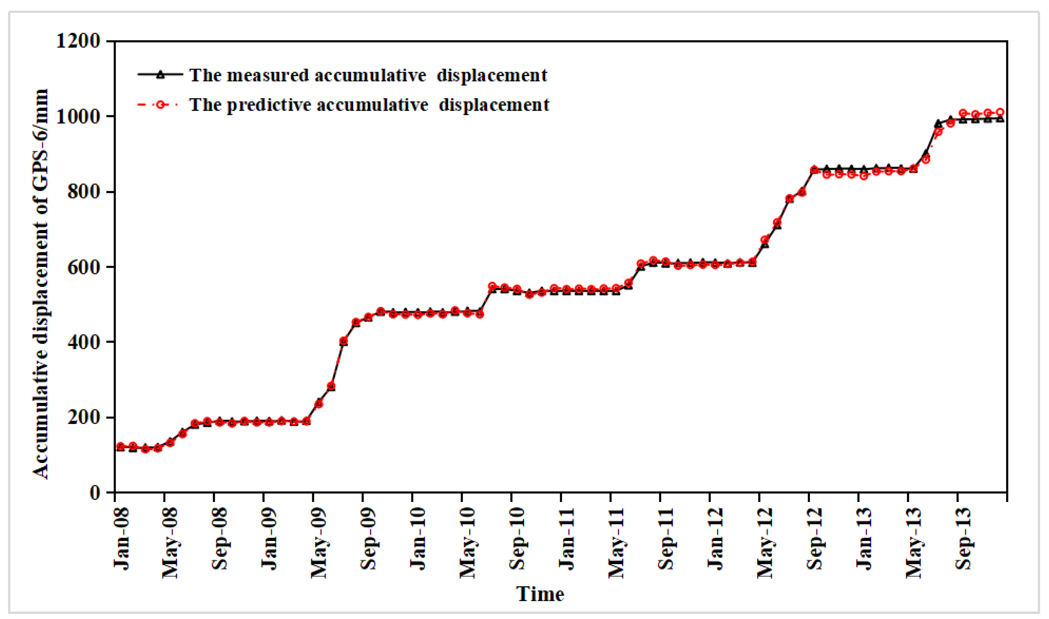
4.3. Prediction of the Accumulative Displacement

The predicted cumulative displacement can be obtained by superposing the predicted trend displacement with the predicted periodic displacement. The monitoring data of the GPS-6 and GPS-3 observation points in the Caojiatuo landslide and the predicted results of the GWO-ELM model are shown in Figure 17 and Figure 18, respectively. The predicted trend displacement and periodic displacement are highly accurate, so the predicted values of accumulative displacement are also highly consistent with the measured ones.

5. Conclusions

The displacement of the Caojiatuo landslide is characterized by step-wise deformation. Based on the analysis of the monitoring data, it is concluded that the precipitation and water level fluctuation in the reservoir area are the key external factors affecting the landslide deformation. External triggering factors cause changes in various hydraulic states of the landslide mass, resulting in sudden and large displacement. Over time, the effects of such factors tend to be stable. Thus, it shows the step-wise-characterized deformation.

Based on the time series theory, the step-wise displacement of the Caojiatuo landslide in the TGR area is divided into trend and periodic displacement by using the moving average method, considering the influence of the internal basic geological conditions (lithology, geological structure, landform and geomorphology, etc.) and the external environmental factors (precipitation, reservoir water level, etc.). The trend and periodic displacement are predicted by polynomial fitting method and GWO-ELM model respectively. These processes have clear physical meaning and is proved to be an effective analytical method.

The GWO-ELM model based on time series theory proposed in this paper can accurately predict the displacement of the Caojiatuo landslide at different stages, such as the creep stage and step deformation stage. It shows a better prediction ability than the nonoptimized ELM model. GWO-ELM model has great application potential in landslide displacement prediction in landslide prone areas such as TGA, and can be used to establish an effective early warning system for geological disasters.

References

1. Pradhan, S.P.; Panda, S.D.; Roul, A.R.; Thakur, M. Insights into the recent Kotropi landslide of August 2017, India: A geological investigation and slope stability analysis. Landslides 2019, 16, 1529–1537. [Google Scholar] [CrossRef]
2. Zhou, W.; Shi, X.; Lu, X.; Qi, C.; Luan, B.; Liu, F. The mechanical and microstructural properties of refuse mudstone-GGBS-red mud based geopolymer composites made with sand. Constr. Build. Mater. 2020, 253. [Google Scholar] [CrossRef]
3. Li, C.; Fu, Z.; Wang, Y. Susceptibility of reservoir-induced landslides and strategies for increasing the slope stability in the Three Gorges Reservoir Area: Zigui Basin as an example. J. Eng. Geol. 2019, 261. [Google Scholar] [CrossRef]
4. Wang, Z.-H.; Li, L.; Zhang, Y.-X. Reinforcement model considering slip effect. J. Eng. Struct. 2019, 198, 109493. [Google Scholar] [CrossRef]
5. Xu, S.; Niu, R. Displacement prediction of Baijiabao landslide based on empirical mode decomposition and long short-term memory neural network in Three Gorges area, China. Comput. Geosci. 2018, 111, 87–96. [Google Scholar] [CrossRef]
6. Carla, T.; Macciotta, R.; Hendry, M.; Martin, D.; Edwards, T.; Evans, T.; Farina, P.; Intrieri, E.; Casagli, N. Displacement of a landslide retaining wall and application of an enhanced failure forecasting approach. Landslides 2018, 15, 489–505. [Google Scholar] [CrossRef] [Green Version]
7. Shinoda, M.; Miyata, Y.; Kurokawa, U.; Kondo, K. Regional landslide susceptibility following the 2016 Kumamoto earthquake using back-calculated geomaterial strength parameters. Landslides 2019, 16, 1497–1516. [Google Scholar] [CrossRef]
8. Guo, F.; Luo, Z.; Li, H.; Wang, S. Self-organized criticality of significant fording landslides in Three Gorges Reservoir area, China. Environ. Earth Sci. 2016, 75. [Google Scholar] [CrossRef]
9. Bao, Y.; Han, X.; Chen, J.; Zhang, W.; Zhan, J.; Sun, X.; Chen, M. Numerical assessment of failure potential of a large mine waste dump in Panzhihua City, China. Eng. Geol. 2019, 253, 171–183. [Google Scholar] [CrossRef]
10. Zhou, C.; Yin, K.; Cao, Y.; Intrieri, E.; Ahmed, B.; Catani, F. Displacement prediction of step-like landslide by applying a novel kernel extreme learning machine method. Landslides 2018, 15, 2211–2225. [Google Scholar] [CrossRef] [Green Version]
11. Hongtao, N. Smart safety early warning model of landslide geological hazard based on BP neural network. Saf. Sci. 2020, 123. [Google Scholar] [CrossRef]
12. Zhang, W.; Xiao, R.; Shi, B.; Zhu, H.-H.; Sun, Y.-J. Forecasting slope deformation field using correlated grey model updated with time correction factor and background value optimization. Eng. Geol. 2019, 260. [Google Scholar] [CrossRef]
13. Miao, S.; Hao, X.; Guo, X.; Wang, Z.; Liang, M. Displacement and landslide forecast based on an improved version of Saito’s method together with the Verhulst-Grey model. Arab. J. Geosci. 2017, 10. [Google Scholar] [CrossRef]
14. Marjanović, M.; Kovačević, M.; Bajat, B.; Voženílek, V. Landslide susceptibility assessment using SVM machine learning algorithm. Eng. Geol. 2011, 123, 225–234. [Google Scholar] [CrossRef]
15. Du, J.; Yin, K.; Lacasse, S. Displacement prediction in colluvial landslides, Three Gorges Reservoir, China. Landslides 2012, 10, 203–218. [Google Scholar] [CrossRef]
16. Polykretis, C.; Ferentinou, M.; Chalkias, C. A comparative study of landslide susceptibility mapping using landslide susceptibility index and artificial neural networks in the Krios River and Krathis River catchments (northern Peloponnesus, Greece). Bull. Eng. Geol. Environ. 2014, 74, 27–45. [Google Scholar] [CrossRef]
17. Lian, C.; Zeng, Z.; Yao, W.; Tang, H. Multiple neural networks switched prediction for landslide displacement. Eng. Geol. 2015, 186, 91–99. [Google Scholar] [CrossRef]
18. Pradhan, B. A comparative study on the predictive ability of the decision tree, support vector machine and neuro-fuzzy models in landslide susceptibility mapping using GIS. Comput. Geosci. 2013, 51, 350–365. [Google Scholar] [CrossRef]
19. Chousianitis, K.; Del Gaudio, V.; Kalogeras, I.; Ganas, A. Predictive model of Arias intensity and Newmark displacement for regional scale evaluation of earthquake-induced landslide hazard in Greece. Soil Dyn. Earthq. Eng. 2014, 65, 11–29. [Google Scholar] [CrossRef]
20. Li, H.; Xu, Q.; He, Y.; Fan, X.; Li, S. Modeling and predicting reservoir landslide displacement with deep belief network and EWMA control charts: A case study in Three Gorges Reservoir. Landslides 2019, 17, 693–707. [Google Scholar] [CrossRef]
21. Huang, F.; Huang, J.; Jiang, S.; Zhou, C. Landslide displacement prediction based on multivariate chaotic model and extreme learning machine. Eng. Geol. 2017, 218, 173–186. [Google Scholar] [CrossRef]
22. Jeddi, S.; Sharifian, S. A hybrid wavelet decomposer and GMDH-ELM ensemble model for Network function virtualization workload forecasting in cloud computing. Appl. Soft Comput. 2020, 88. [Google Scholar] [CrossRef]
23. Huang, G.-B. An Insight into Extreme Learning Machines: Random Neurons, Random Features and Kernels. Cogn. Comput. 2014, 6, 376–390. [Google Scholar] [CrossRef]
24. Reichenbach, P.; Rossi, M.; Malamud, B.D.; Mihir, M.; Guzzetti, F. A review of statistically-based landslide susceptibility models. Earth-Sci. Rev. 2018, 180, 60–91. [Google Scholar] [CrossRef]
25. Mirjalili, S.; Mirjalili, S.M.; Lewis, A. Grey Wolf Optimizer. Adv. Eng. Softw. 2014, 69, 46–61. [Google Scholar] [CrossRef] [Green Version]
26. Jaafari, A.; Panahi, M.; Pham, B.T.; Shahabi, H.; Bui, D.T.; Rezaie, F.; Lee, S. Meta optimization of an adaptive neuro-fuzzy inference system with grey wolf optimizer and biogeography-based optimization algorithms for spatial prediction of landslide susceptibility. Catena 2019, 175, 430–445. [Google Scholar] [CrossRef]
27. Yang, B.; Yin, K.; Lacasse, S.; Liu, Z. Time series analysis and long short-term memory neural network to predict landslide displacement. Landslides 2019, 16, 677–694. [Google Scholar] [CrossRef]
28. Wang, X.; Han, M. Online sequential extreme learning machine with kernels for nonstationary time series prediction. Neurocomputing 2014, 145, 90–97. [Google Scholar] [CrossRef]
29. Huang, G.B.; Wang, D.H.; Lan, Y. Extreme learning machines: A survey. Int. J. Mach. Learn. Cybern. 2011, 2, 107–122. [Google Scholar] [CrossRef]
30. Zhang, Y.; Zhang, Z.; Xue, S.; Wang, R.; Xiao, M. Stability analysis of a typical landslide mass in the Three Gorges Reservoir under varying reservoir water levels. Environ. Earth Sci. 2020. [Google Scholar] [CrossRef]
31. Zhang, Y.; Zhu, S.; Zhang, W.; Liu, H. Analysis of deformation characteristics and stability mechanisms of typical landslide mass based on the field monitoring in the Three Gorges Reservoir, China. J. Earth Syst. Sci. 2018, 128. [Google Scholar] [CrossRef] [Green Version]
32. Xu, C.; Sun, Q.; Yang, X. A study of the factors influencing the occurrence of landslides in the Wushan area. Environ. Earth Sci. 2018, 77. [Google Scholar] [CrossRef]
33. Cao, Y.; Yin, K.; Alexander, D.E.; Zhou, C. Using an extreme learning machine to predict the displacement of step-like landslides in relation to controlling factors. Landslides 2015, 13, 725–736. [Google Scholar] [CrossRef]
34. Tan, F.; Hu, X.; He, C.; Zhang, Y.; Zhang, H.; Zhou, C.; Wang, Q. Identifying the Main Control Factors for Different Deformation Stages of Landslide. Geotech. Geol. Eng. 2017, 36, 469–482. [Google Scholar] [CrossRef]
35. Yu, S.; Zhang, J.; Ren, X. Numerical Analysis of the Seepage Characteristics of Slopes with Weak Interlayers under Different Rainfall Levels. Appl. Ecol. Env. Res. 2019, 17, 12465–12478. [Google Scholar] [CrossRef]
36. Qiu, L.; Song, D.; He, X.; Wang, E.; Li, Z.; Yin, S.; Wei, M.; Liu, Y. Multifractal of electromagnetic waveform and spectrum about coal rock samples subjected to uniaxial compression. Fractals 2020, 28, 2050061. [Google Scholar] [CrossRef]
37. Bao, Y.; Zhai, S.; Chen, J.; Xu, P.; Sun, X.; Zhan, J.; Zhang, W.; Zhou, X. The evolution of the Samaoding paleolandslide river blocking event at the upstream reaches of the Jinsha River, Tibetan Plateau. Geomorphology 2020, 351, 106970. [Google Scholar] [CrossRef]
38. Liu, X.; Cai, G.; Liu, L.; Liu, S.; Puppala, A.J. Thermo-hydro-mechanical properties of bentonite-sand-graphite-polypropylene fiber mixtures as buffer materials for a high-level radioactive waste repository. Int. J. Heat Mass Tran. 2019, 141, 981–994. [Google Scholar] [CrossRef]
39. Rong, X.; Zheng, S.; Zhang, Y.; Zhang, X.; Dong, L. Experimental study on the seismic behavior of RC shear walls after freeze-thaw damage. Eng. Struct. 2020, 206, 110101. [Google Scholar] [CrossRef]
40. Meng, T.; Xie, J.; Yue, Y. Experimental study on the evolutional trend of pore structures and fractal dimension of low-rank coal rich clay subjected to a coupled thermo-hydro-mechanical-chemical environment. Energy 2020, 203, 117838. [Google Scholar] [CrossRef]
41. Li, Y.; Wei, M.; Liu, L.; Xue, Q.; Yu, B. Adsorption of toluene on various natural soils: Influences of soil properties, mechanisms, and model. Sci. Total Environ. 2020. [Google Scholar] [CrossRef]
42. Ma, G.; Hu, X.; Yin, Y.; Luo, G.; Pan, Y. Failure mechanisms and development of catastrophic rockslides triggered by precipitation and open-pit mining in Emei, Sichuan, China. Landslides 2018, 15, 1401–1414. [Google Scholar] [CrossRef]
43. Zhou, Y.; Zhao, D.; Tang, Q.; Wang, M. Experimental and numerical investigation of the fatigue behaviour and crack evolution mechanism of granite under ultra-high-frequency loading. Roy. Soc. Open Sci. 2020, 7, 200091. [Google Scholar] [CrossRef] [PubMed] [Green Version]
44. Li, L.; Wu, W.; El Naggar, M.; Mei, G.; Liang, R. Characterization of a jointed rock mass based on fractal geometry theory. Bull. Eng. Geol. Environ. 2019, 78, 1234. [Google Scholar] [CrossRef]
45. Li, Z.W.; Yang, X.L.; Li, T.Z. Static and seismic stability assessment of 3D slopes with cracks. Eng. Geol. 2020, 265, 105450. [Google Scholar] [CrossRef]
46. Liu, F.; Yi, J.; Cheng, P.; Yao, K. Numerical simulation of set-up around shaft of XCC pile in clay. Geomech. Eng. 2020, 21, 489–501. [Google Scholar]
47. Yan, G.; Shen, Y.; Gao, B.; Zheng, Q.; Fan, K.; Huang, H. Damage evolution of tunnel lining with steel reinforced rubber joints under normal faulting: An experimental and numerical investigation. Tunn. Undergr. Space Technol. 2020, 97, 103223. [Google Scholar] [CrossRef]
Figure 1. Framework system of the Extreme Learning Machine with Gray Wolf Optimization (GWO-ELM) prediction model.
Water 12 01860 g001
Figure 2. Locations of the Caojiatuo landslide.
Water 12 01860 g002
Figure 3. Geomorphological map of the Caojiatuo landslide with monitoring network [17].
Water 12 01860 g003
Figure 4. Cross section along the II-II’ profile of the Caojiatuo landslide [17].
Water 12 01860 g004
Figure 5. Relationship of accumulative displacement, reservoir level and precipitation in the Caojiatuo landslide.
Water 12 01860 g005
Figure 6. The measured trend and periodic displacements of GPS-6 in the Caojiatuo landslide.
Water 12 01860 g006
Figure 7. The measured trend and periodic displacements of GPS-3 in the Caojiatuo landslide.
Water 12 01860 g007
Figure 8. Comparison of the predictive trend displacement and the measured of GPS-6.
Water 12 01860 g008
Figure 9. Comparison of the predictive trend displacement and the measured of GPS-3.
Water 12 01860 g009
Figure 10. Relationship between precipitation and the measured periodic displacement in the last one and two months. (a) Dataset of GPS-6, (b) Dataset of GPS-3.
Water 12 01860 g010
Figure 11. Relationship between monthly change and the measured periodic displacement in the last one month. (a) Dataset of GPS-6, (b) Dataset of GPS-3.
Water 12 01860 g011
Figure 12. Gray relational grade between the accumulative landslide displacement and evolution stage in recent months.
Water 12 01860 g012
Figure 13. Comparison of the predictive periodic displacement and the measured of GPS-6 between 2008 to 2012.
Water 12 01860 g013
Figure 14. Comparison of the predictive periodic displacement and the measured of GPS-3 between 2008 to 2012.
Water 12 01860 g014
Figure 15. Comparison of the predictive results of monitoring point GPS-6 predicted by GWO-ELM and ELM models.
Water 12 01860 g015
Figure 16. Comparison of the predictive results of monitoring point GPS-3 predicted by GWO-ELM and ELM models.
Water 12 01860 g016
Figure 17. Comparison of the predictive accumulative displacement and the measured of GPS-6.
Water 12 01860 g017
Figure 18. Comparison of the predictive accumulative displacement and the measured of GPS-3.
Water 12 01860 g018