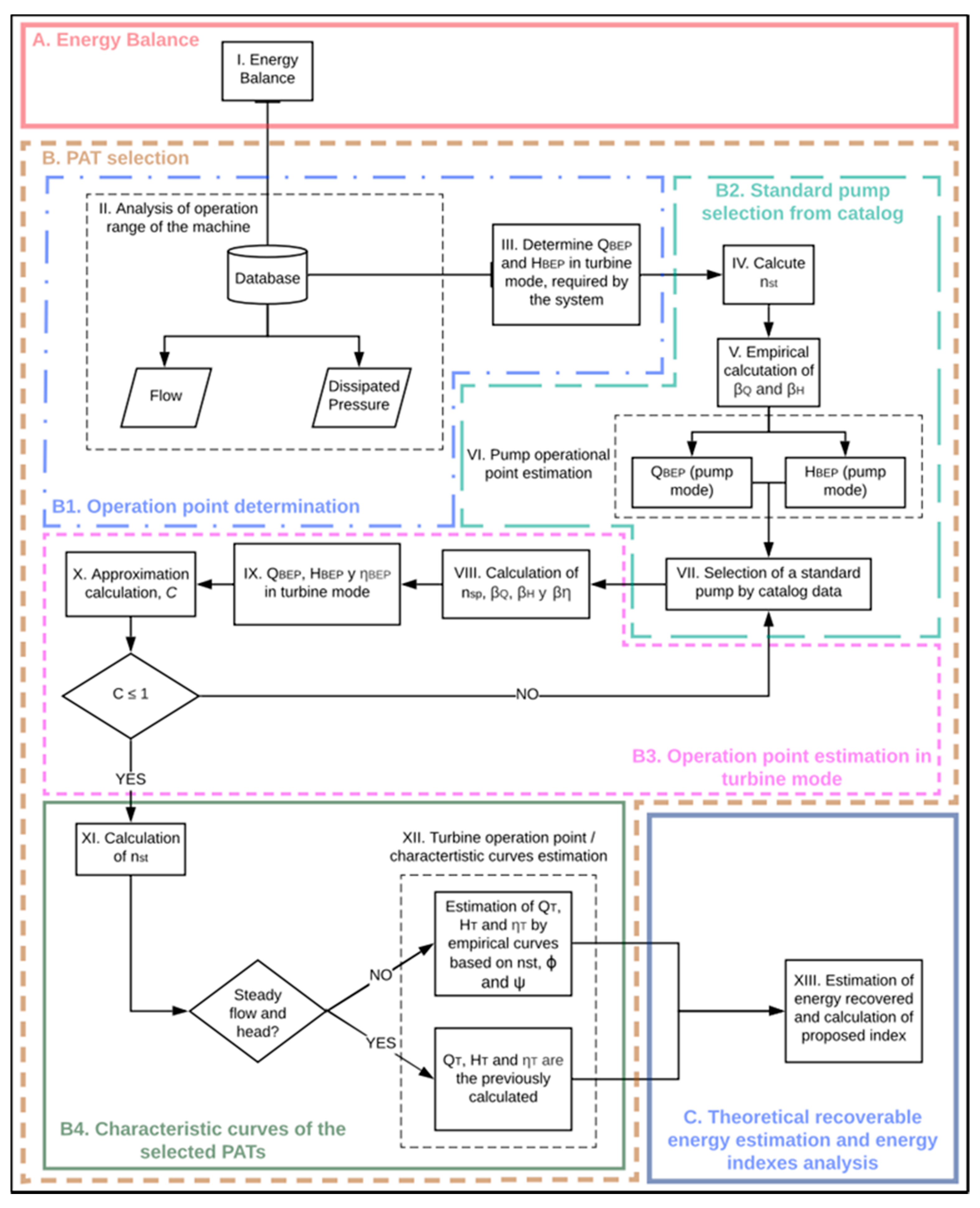
Article

Applied Strategy to Characterize the Energy Improvement Using PATs in a Water Supply System

by
Luis E. Camilo Rosado
1,
P. Amparo López-Jiménez
1,
Francisco-Javier Sánchez-Romero
2,
Pilar Conejos Fuertes
3 and
Modesto Pérez-Sánchez
1,*
1
Hydraulic and Environmental Engineering Department, Universitat Politècnica de València, 46022 Valencia, Spain
2
Rural and Agri-food Engineering Department, Universitat Politècnica de València, 46022 Valencia, Spain
3
EMIMET C/Pedrapiquers, 4 Pol. Ind. Vara de Quart, 46014 Valencia, Spain
*
Author to whom correspondence should be addressed.
Water 2020, 12(6), 1818; https://doi.org/10.3390/w12061818
Submission received: 9 June 2020 / Revised: 18 June 2020 / Accepted: 22 June 2020 / Published: 24 June 2020
(This article belongs to the Special Issue Hydraulic Dynamic Calculation and Simulation)

Abstract

:
Sustainable development has been an idea raised in recent years. The results are related to the improvement and the use of new technologies to maximize efficiency in water management. However, energy consumption has been increasing as a consequence of new management and uses of water. Especially in pressurized water distribution systems, the use of pressure reduction valves (PRVs) increases the water usage efficiency but it decreases the energy consumption efficiency, since the valves dissipate energy that could be recovered. This research presents a proposal of a recovery system based on the installation of pumps used as turbines (PATs). These machines are located in different points of the high-pressure water distribution system in the Valencia Metropolitan System (Spain). An annual estimate of the theoretical recoverable energy as well as the “ideal” pump for each point were proposed. The theoretical recovered energy value was 847,301 kWh/year for a specific analyzed point. Besides, the characteristic curves of the PATs from a selected point were determined, estimating an improvement in the sustainable indexes. The calculus of these green parameters showed that the implementation of this solution caused a reduction in consumed energy of 1.50 kWh/m3.

1. Introduction

Water supply distribution systems have a fundamental objective: assuring the availability of water in the desired quantity and the required quality to satisfy the health parameter. To fulfill this intent, urban distribution systems depend on a great amount of energy to supply the water at a minimum pressure for it to be rightly used.
Energy has always been considered an important factor in society. Its significance has grown pressingly in recent years. This is due to the uncontrolled increase in the world population, the concentrations in urban cities and the rise in the demand of resources such as water and energy which threaten to force a future global deficit in natural resources [1].
In the water sector, the water-energy nexus has constantly been an important issue, since one of the most energy-consuming activities in a city is the cycle of water consumption. However, water supply and distribution are services which must be provided to the population as an obligation, since it is a right that concerns everyone. Therefore, water managers have continuously tended to find ways to enhance their systems. These strategies are focused on looking for approaches to have economic and sustainable development [2].
Water distribution systems consume different amounts energy around the world. This consumption depends on the topography and topology of the water network mainly. As an example, the water cycle represented around 7% of the total energy consumption in Spain in 2010. A total of 20% of the energy used for the water cycle was employed in the distribution of water to the consumption points in the different sectors [2]. Particularly in the city of Valencia (Spain), the energy consumption was 53.21 GWh/year when the water cycle was considered in 2009. This value can be normalized to 1124 kWh/m3 when the water consumption was considered. The catchment, potabilization and distribution of water represented 30% of the energy used for the water cycle in Valencia [3].
Water distribution serves as the one phase of the water cycle, which consumes the most energy. Therefore, this phase is the broadest to improve the efficiency indexes. Undoubtedly, one of the easiest methods to reduce the energy required for water distribution is pressure management. If the pressure is low in the system, it has less leaks, thus the flow decreases as well as the energy input. There are three basic methods to achieve pressure management. These operational strategies are described in Table 1.
Water distribution systems mostly depend on energy [13]. This connection between water and energy creates a nexus, being part of the near-future sustainable development main consideration. In this framework, the use of small and micro-hydropower systems (specially using pumps working as turbines—PAT) has been increasing in recent years. PATs have demonstrated to be a feasible solution to recover the potential energy in water systems, both urban [14,15] and irrigation [16]. This pump’s feasibility is linked to economic, availability and construction criteria. Theoretically, all types of pumps could be used in water systems [17,18]. However, when the water managers choose a PAT, it is advisable to avoid choosing axial pumps since these are less efficient than radial machines [19]. In addition, the axial pumps are the machines that have had fewer experiments in this regard and therefore, the efficiency prediction is most difficult [13].
This research establishes a strategy to choose PATs according to the methodology proposed by [20]. The novelty of this manuscript is that it was applied using data from pairs (i.e., flow and pressure) of the real water systems. Therefore, the proposed energy analysis, the selection of the machines as well as the comparison between different scenarios were applied to reality. This research aims to estimate the potentially recoverable energy of the supply network at the chosen study point as well as the selection of the machines to be used in those points. This selection was based on a manufacturer catalogue of pumps. For a specific case study point, the complete hydraulic design was made in order to approximate, in a more precise way, the recoverable energy in addition to the calculation of the proposed sustainability indicators to compare the impact the installation of PATs has on the system.

2. Materials and Methods

2.1. Materials

This manuscript aims to analyze several chosen points from the high-pressure water distribution system, which is called the Valencia Metropolitan System (VMS) in Spain. Those points have PRVs operating at the moment to try and maintain a steady pressure throughout the network. The pressure values upstream and downstream of the valves at each point are registered with an interval of 10 min, alongside with the date and the flow. Using these data available, one can only calculate the theoretical recoverable energy (ETR) and the theoretical unrecoverable energy (ENTR). The available data consist of more than 50,000 entries for variables of date, flow (Q), upstream (Pu) and downstream pressure (Pd) for each of the chosen study points. They are the results of the data registered from a PRV installed at every case, with a time interval between each entry of 10 min. The used data considered one year from January to December. Really, the operational conditions are similar each year because the water system case-studied is the main distribution ring. This network distributes the different origin resources to the different municipalities where there are other tanks and pipes, which supply to users.
Table 2 exemplifies the data available for each study point. The meaning of every column of data is:
  • Time (∆t = 10 min) is the date when the data were registered, they are in dd-mm-yy hh:mm format with 10 min of interval;
  • Q is the instant flow registered at the date, measured in liters per second (L/s);
  • P u is the pressure upstream of the valve registered at the date, measured in meters of water column (m w.c.);
  • P d is the pressure downstream of the valve registered at each time (m w.c.). This is the setting value, which should be established to guarantee the pressure conditions in the water supply system. The valves are chosen to keep the pressure head close to the setting.

2.2. Strategy to Characterize the PAT Systems, Estimating the Improvement of Energy Indexes

Figure 1 describes the proposed methodology, which was followed in this research. It is focused on the selection of the PAT for each analyzed point, highlighting two important analyses to be made: the energy balance and the estimation of the theoretical recoverable energy. Besides, the plan establishes the operation strategy when the system operates considering hydraulic regulation.
The procedure is integrated on three main blocks: A. energy balance, B. PATs selection and C. theoretical recoverable energy estimation and analysis of energy indexes. These blocks are described in the next subsections.

2.2.1. Energy Balance (A) for the Supply Network at the Chosen Study Points

The first block (Figure 1) is an energy balance (Step I). It aims to determine the total energy supplied to the system while differentiating the required energy for the proper water consumption from the energy loss, which could be either operational losses or structural losses [21].
The proposed energy balance to quantify the theoretical recoverable energy is based on the energy distribution plan shown in Figure 2. The difference between piezometric lines can be observed in Figure 2a (without PAT) and Figure 2b (considering PAT).
The energies that define the scheme presented below are described as follows [16]:
Total energy (ET): total energy to the system when the consumption is null in the entire network. It corresponds to the static energy of the network;
Friction energy (EFR): for an interval time, it is the friction dissipated energy in the network from its outing point to the analyzed point;
Theoretical energy necessary (ETN): this is the lowest possible energy to fulfil the local minimum pressure requirements in the least favorable point in the network;
Energy required for consumption (ERI): this is the required energy to ensure the local minimum pressure requirements for a time interval in the analyzed point (ETN ≥ ERI);
Theoretical available energy (ETA): this is the available energy for recovery in an analyzed point. It also equals to the sum of the theoretical energy recoverable (ETR) plus the theoretical energy unrecoverable (ENTR);
Theoretical recoverable energy (ETR): this is the maximum theoretical recoverable energy in an analyzed point ensuring that the local minimum pressure requirements are met at the downstream;
Theoretical unrecoverable energy (ENTR): this is the energy in an analyzed point that cannot be recovered. This energy is necessary to ensure the minimum pressure in the most unfavorable consumption node.
The values for each of the previous energies described are defined by the expression presented in Table 3. These terms were defined by [5].
Where subscript “i” indicates each analyzed point; Qi is the flow circulating by a line (m3/s); and zi is the geometry level above the reference plane of the analyzed point. In this case, the reference is sea level (m); z0 is the geometry level above the reference plane of the free water surface of the reservoir. In this case as well, the reference is sea level (m); ∆t is the time interval (s); Pi is the service pressure in the analyzed point when consumption exists (m w.c.); Pmin i is the minimum pressure of service of an analyzed point to ensure the minimum in the most disadvantageous consumption node (m w.c.); Pmin C is the minimum pressure of service of an analyzed point required by the local authorities, this value is set to be 25 m w.c. in VMS; and Hi is the head in the analyzed point (m w.c.), obtained as H i = P i max ( P min i ; P min C ) .
This information is used to calculate the total instant power supplied to the analyzed point defined by the following equation:
P W t i n s t   i   ( k W ) = 9.81 1000 Q i P u ,   i η
where Qi is the flow circulating by the valve in L/s; and η is the efficiency of the turbine. It is a value between 0 and 1. For estimation purposes, an efficiency of 1 is selected; Pu is the pressure upstream of the PRVs. It is measured in meters of water column (m w.c.).
In a similar calculus, the theoretical recoverable instant power is estimated for the analyzed point with the next equation:
P W r i n s t   i   ( k W ) = 9.81 1000 Q i H   i η
where η is the efficiency of the turbine. It is a value between 0 and 1. For estimation purposes and comparison, efficiencies of 1 and 0.6 have been selected; Hi is the dissipated pressure by the PRVs. It is obtained by the difference between P u and P d measured in m w.c.
When P W r is known, the total energy supplied to the analyzed point is calculated using the next equation:
E T i ( k W h ) = 9.81 3600 · Q i · P u   i · Δ t = P W t i n s t   i Δ t 3600
where ∆t is the time interval (s).
Subsequently, the theoretical recoverable energy is estimated by the following equation:
E T R i ( k W h ) = 9.81 3600 · Q i · H i · Δ t = P W r i n s t   i Δ t 3600
Having determined the previous values, the theoretical unrecoverable energy is estimated. The value is defined by the following equation:
E N T R i ( k W h ) = E T A i E T R i
To ease the analysis, and for better understanding of the data, the results are grouped in time intervals of 1 h, 24 h, 1 month and 1 year.

2.2.2. Selection of PATs for Each Study Case (B)

The implementation of PATs in a water distribution system is widely justified by many advantages such as the ability to recover energy from the network, the decrease in the carbon footprint, the lower investment cost (compared to the installation of a traditional turbine), the readily available pumps and spare parts and the simplicity of the system [13].
However, the use of this technology has been depleted by the lack of characteristic curves for the pumps working as turbines. The absence of these curves creates an uncertainty in the design of the energy recovery systems. Although the right methodology is to ask the manufacturers for the curves of the machine working in reverse or to carry out experimentation in a laboratory to obtain these curves, this is not common because knowledge of curves is difficult to achieve. Usually, the design is based on empirical methods developed through the year. The following figure illustrates the methodology used in this paper:
The block “B” is divided on four main course procedures derived from Figure 1. These are: (B-1) determinate the theoretical best efficiency point (QBEP,T, HBEP,T) for the ideal PAT at an analyzed point (steps II and III); (B-2) select a standard water pump by the catalog data that matches the requirement for energy recovery at the analyzed point (steps IV to VII); (B-3) estimate the operation point of the machine in turbine mode, based on the manufacture’s data in pump mode (steps VIII to X); and (B-4) approximate the characteristic curves of the selected PAT by the proposed empirical curves (steps XI and XII).

B-1. Determination of the Theoretical Best Efficiency Point

The analysis of the operation range depends on a detailed statistical study. For each of the eight different study points, there are more than 50,000 entries for every variable (date, flow, upstream pressure and downstream pressure). A high variability for the values is expected, due to the great amount of data available and the time length of the series. As a result, the best efficiency point is the most representative operation point of the data series. To determine the most typical flow and the dissipated pressure in the analyzed point, a statistical study was based on the use of histograms for each variable (flow and head).
A fruitful technique, which is based on programming, was developed in this manuscript in order to be used to enhance the precision of the selection of the most characteristic variable. This was to delimitate the data to the desired work zone and repeat the process of the histogram and scatter plots.

B-2. Selection of a Standard Water Pump by Catalog Data

The PAT selection is based on the methodology, which is proposed in Figure 1. The steps are the following: (IV) calculate the specific speed for the “ideal” turbine for the analyzed point; (V) determination of the coefficients to adapt the previous operational point as a turbine to a best efficiency point as a pump; (VI) estimate the best efficiency point (BEP) for the required machine in pump mode, using the previous coefficients; and (VII) select the standard pump from the available machines in the market based on the estimated BEP.
The first three steps mentioned above are to estimate the operational point for the standard water pump that matches the requirement previously established for a specific analyzed point. The head to be recovered by a machine in turbine mode does not match with the head for the same machine in pump mode [13]. The estimation of the behavior of pumps in their turbine mode has been an important issue and has led to numerous studies. Unfortunately, most of the studies did not have enough pumps for experimentation and therefore their results lack a certain precision [20]. The proposed strategy uses both Pérez-Sánchez et al.’s method and other proposed methods for comparison and validation.

B-3. Estimate the Operation Point of the Machine in Turbine Mode

Three steps are considered in this sub-phase according to Figure 1: (VIII) determine the BEP from the catalog of the selected pump, estimating the conversion factors to transform the BEP in pump mode to a BEP in turbine mode; (IX) estimate the best efficiency point for the machine as a turbine by the previous coefficients; (X) calculate the approximation of C value. A valid selection must have a value of C ≤ 1.
The characteristics curves of a machine can be defined by polynomial equations depending on the specific speed (ns) of the machine. When there is only a suction pipe, this value is used to classify either pumps ( n S P ) or pumps in turbine mode ( n S T ). These values are determined by the following expressions [20]:
n S P = n Q B E P , P H B E P , P 3 / 4
n S T = n Q B E P , T H B E P , T 3 / 4
where QBEP,P is the flow in the best efficiency point in m3/s when the machine operates as a pump, HBEP,P is the head in the best efficiency point in m w.c. when the machine operates as a pump, QBEP,T is the flow in the best efficiency point in m3/s when the machine operates as a turbine, HBEP,T is the head in the best efficiency point in m w.c. when the machine operates as a turbine and n is the rotational speed in rpm.
Previous research [20] proposed the following empirical relationship to define the best efficiency point of the machine as a function of the specific speed (Table 4):
These values are used to estimate a flow, head or efficiency of the machine working as a pump or as a turbine, based on the same variables when the machine is working in the opposite way. They are applied in the following equations:
Q B E P , T = β Q · Q B E P , P
H B E P , T = β H · H B E P , P
η B E P , T = β η · η B E P , P
where βQ is the conversion coefficient for the flow, βH is the conversion coefficient for the head and βη is the conversion coefficient for efficiency.
This research also includes the empirical equations proposed in previous studies to compare errors. These formulas are summarized in Table 5:
The criteria to accept the pump selected is based on calculating an approximation value between the estimated best efficiency point of the machine in turbine mode and the theoretical best efficiency point determined for the analyzed point. The concept is based in an ellipse form which enables an error varying from ± 30% at the major axis and ± 10 at the minor axis for both the flow and head. The approximation value must be C ≤ 1, and the value is defined by the following equation [20]:
C 2 = ( 1 2 ( Δ q + Δ h ) 0.3 ) 2 + ( 1 2 Δ q 2 + Δ h 2 2 Δ q Δ h 0.1 ) 2

B-4. Estimation of Characteristic Curve of PATs from Empirical Curves

This last sub-phase related to PAT selection considers the steps XI and XII from Figure 1. The goal of this sub-phase is to estimate the characteristic curves of PATs, [20] proposed curves as function of the nondimensional numbers of discharge (φ) and the head (ψ) defined by the following equations.
φ = Q t n   D 3
ψ = g   H t n 2   D 2
π = P t ρ   n 3   D 5 = φ   ψ   η t
where D is the impeller diameter in m, g is the gravity constant in m/s2, Pt is the shaft power in the PAT, ηt is the efficiency of the PAT and n is the rotational speed in rps.
The empirical curves mentioned as a function of the nondimensional numbers of discharge and head, as well as the specific speed of the test pumps, returns estimate curves of Qt-Ht and Qtt. They are presented in Figure 3a,b.
Lastly, two other curves are needed for the regulation of the PATs. The runaway curve, which consists of the curve Q-H of a PAT for which the power output is zero and the zero-speed curve, of the machine. They are defined by the following equations [20]:
k R u n a w a y = ( 6.83008 n s t ) 2
H R u n a w a y = k R u n a w a y   Q t 2
k z e r o s p e e d = ( 4.36583 n s t ) 2
H z e r o s p e e d = k z e r o s p e e d   Q t 2
where HRunaway is the head in m w.c. at which the machine runs with a power output of zero; kRunaway is the coefficient proposed by Pérez-Sánchez et al.; Hzero-speed is the head in m w.c. while the rotational speed is zero; and kzero-speed is the coefficient proposed by Pérez-Sánchez et al. (2020).

2.3. Estimation of Theoretical Recoverable Energy and Calculation of Sustainability Indicators

Once the characteristic curves from the chosen PATs were known for an analyzed point, a more precise theoretical recoverable energy estimation was made. The characteristics curves were meant to be used to evaluate the hydraulic efficiency of the recovery system. However, this research considers the electrical efficiency of the generator for a more realistic approximation since the electric generator efficiency has a great significance on the global efficiency of the machine when hydraulic and electrical machines are considered [31]. The efficiency used for the electric generator represents the lowest permitted efficiencies in the marked motors associated to the IE code. They are defined by IEC/EN 60034-30-1 [32]. It has four different classes of motor: IE4 Super-Premium efficiency, IE3 Premium efficiency, IE2 High efficiency and IE1 Standard efficiency. This manuscript chose the IE1 motor, which varies as a function of the power. A common practice to increase the recovered energy is to install a variable frequency drive for the machines. However, for this estimation, a variable frequency drive was not considered for the installed PATs as the worst-case scenario is being analyzed.
An energy balance is repeated after the implementation of the energy recovery system to compare the existing conditions to the post-solution condition. The sustainable indicators shown in Table 6 are meant to reveal the changes connected to the installation of the PATs and it helps to assess the performance of the water distribution system against a sustainable focus [33].
This research proposes the sustainability indicators for pressurized water systems recommended by [34]. These indicators emphasize the focus on the energetic and environmental development for these systems. Two other indicators were proposed. They are based on the previously mentioned indicators. They were the absolute annual consumed energy (IAAE) and the absolute consumed energy per unit volume (IAEFW). These indicators present better the reduction in needed energy in a system where the recovered energy is being consumed.

3. Results

3.1. Case Study Description

This research featured eight different network points from the high-pressure water distribution system of VMS in Spain. The available data were an annual series related to flow, upstream pressure and downstream pressure from an installed pressure reducing valve at each point, referenced to a piece of date information with an interval of 10 min.
The water distribution network of VMS is schemed in Figure 4, highlighting the study points of the system. The points between 1 and 5 are presented in Figure 4a and the remaining points are presented in Figure 4b. The legend from the figure specifies the color code to differentiate each one of them through the continuing length of the study.
Figure 5 summarizes the irregularity of the data. A high variability can be observed. This is because there are more than 50,000 entries for each variable and the water system operated under demand:

3.2. Theoretical Recoverable Energy Estimation

Based on the mentioned methods, the theoretical recoverable energy is estimated for two different scenarios:
  • Ideal efficiency (η = 100%): an ideal and practically unreachable scenario, it is used as a reference to compare the ETR and the approximation made after the PATs are selected;
  • Conservative efficiency (η = 60%): a conservative scenario, using the right PATs selection and the right hydraulic design, this value is likely to be obtained or surpassed.
To ease the comparison, the results of the theoretical recoverable energy estimation were grouped at bigger intervals such as 1 h, 24 h, 1 month and the complete data series of a year length. The results for point #7 are summarized in Table 7 and Table 8:
As shown in the previous tables, a theoretical recoverable energy of 847,301.47 kWh/year was available at point #7, representing 57.35% of the total energy consumed at this point. For a more conservative approach, considering an efficiency of 60%, the theoretical recoverable energy was 508,380.88 kWh/year which represented 34.41% of the total energy consumed at this point. From the difference between the average theoretical recoverable energy monthly and both, the minimum and maximum theoretical recoverable energies were −10.79% and 16.40%, respectively. Therefore, the conditions were fairly stable for the system, facilitating the selection for a PAT.
The same estimations were made for each study. Figure 6 compares the percentage of theoretical recoverable and unrecoverable energy for each point:
Figure 6 highlights that points such as #1, #2 and #5 consumed more than 1,000,000 kWh/year but their theoretical recoverable energy was at maximum equal to 50%. However, point #2 had the largest amount of theoretical recoverable energy. In contrast, point #3 presented the highest percentage of ETR (above 70%) for a total of 1,055,420 kWh/year.

3.3. Most Representative Operational Point Estimation

For each point, a preliminary statistical analysis was made. The results of the analysis for point #7 are presented in Figure 7d. Following the proposed methodology, Figure 7a,b shows the flow and head histograms, respectively.
When point #7 was analyzed, the registered flow was concentrated in two main ranges: (i) 45–60 L/s and (ii) 390–405 L/s (Figure 7a). Both ranges tended to operate for different heads, which are shown in Figure 7c. Therefore, if the recovery systems want to be defined for this point, two PATs groups were selected with one of the groups consisting of two PATs working in parallel.
A representative operational point was determined for the PATs to be installed in the system for each analyzed point. Some points would have various operational points as the hydraulic design contemplates different PATs groups to optimize the recoverable energy available for the specific point. The used criterion to choose the PAT considered the frequency histogram of the flow and head for each machine. Different iterations were checked using programming to choose the best point. The results are summarized in Table 9.
Figure 8 highlights the graphical classification for the PATs of each point. This was based on the proposed general range of application of different turbine types. The standard pump was selected from the catalog data available in the market, looking for the type of machine specified in the previously mentioned image.

3.4. PATs Selection

Point #7 had two PATs groups with different characteristics, the conversion for both operational points will be presented in the same table. Table 10 offers a summary of the operational point for either of the groups.
Based on those points, the best efficiency point was estimated comparing different methods. The results are presented in Table 11.
Using the prior estimated BEP, the selection of standard pumps that matched these requirements was made. The selected pumps, which were chosen using manufacturer catalogs [33,34], and their best efficiency points are shown in Table 12.
Having selected the pumps for the groups of point #7, the transformation from BEP as a standard pump to a BEP in turbine mode was made. The results of the coefficients calculation and the BEP for each group are presented in the Table 13 and Table 14.
Both PATs meet the selection criteria for every method of estimation, except for the Alatorre-Frenk one, where the C value was 1.38. However, the main method used for this manuscript was the proposed method by [20]. This approximation presented good C values, which were 0.14 and 0.07 for group 1 and group 2, respectively. The same methodology was performed for each case of study. Table 15 presents the selected pumps for each analyzed point along with their best efficiency point as a standard pump. In addition, it shows the BEP estimation in turbine mode once the pump was selected. The pumps were chosen using manufacturer catalogs [34,35,36,37].

3.5. Estimation of PATs Characteristic Curves by Empirical Method

As previously mentioned, the following sections depend solely on the data from point #7, although they can be applied to the rest of the points. The empirical methodology proposed by Pérez-Sánchez et al. is based on three variables: (1) non-dimensional discharge number (φ); (2) non-dimensional head number (ψ); and (3) specific speed for the pump used as a turbine ( n s T ). These variables for the selected machine are presented in Table 16.
Using the earlier values, the empirical curves were selected to estimate the values for the characteristic curves of each PAT (Figure 3). The curves, which were defined by the specific speed of nsT = 38.49 and nsT = 40.85, were used to interpolate the required curve defined by n s T = 39.47.
Based on these curves, the characteristic curves for the PATs from point #7 were obtained. Figure 9 shows the estimation of the curve for both selected machines at point #7. The operational curve is defined considering the machines operate a uniform rotational speed. The minimum and maximum operational flows are defined in the Figure 9.
The characteristic curves for group 1 are defined by the following equations:
  • The head and efficiency for flows lower than 60 L/s are obtained by these equations:
H t = 15.048 + 11.55 · 10 3   Q t 2
η t = 2.559 · 10 4   Q t 2 + 34.14 · 10 3   Q t 0.5389
  • For flows higher than 60 L/s, the head and efficiency are obtained by these equations:
H t = 17.662 · 10 3   Q t 2 0.779   Q t + 39.358
η t 0.61 = 1.219 ( Q t 54.55 ) 4 + 6.95 ( Q t 54.55 ) 3 14.578 ( Q t 54.55 ) 2 + 13.231   Q t 54.55 3.383
For group 2, the characteristic curves shown in Figure 9 are defined by the following equations:
H t = 13.415 · 10 4   Q t 2 0.1901   Q t + 26.192
η t = 1.587 · 10 11   Q t 5 + 1.05   · 10 8 Q t 4 2.1   · 10 6   Q t 3 7.68   · 10 6   Q t 2 + 0.04535   Q t 2.967

3.6. Estimation of the Theoretical Recoverable Energy with the Installed PATs

Once the characteristic curves for each PAT installed in the analyzed point were defined, the next step was to estimate the theoretical recoverable energy with the newly selected PATs installed. The theoretical recoverable energy was estimated considering the PAT efficiency curve as a function of the flow (Figure 9). In Figure 10a, a schematic arrangement is presented for the installed pump’s important elements such as: the installed PATs, the PRVs for the bypass and the final regulation.
The pressure reduction valves are that important for the system because they are responsible for the dissipation of the remaining energy in the system. The installation of these valves allows water managers to guarantee the flow and the pressure at the consumption points. The flow variation over time does not have significance if the machine is regulated correctly (when there is variation in the rotational speed) and the pressure reduction valves are defined, installed and controlled by pressure sensors. Another important factor for the estimation is the electric generator. Two scenarios were considered for this matter: (i) variable efficiency as a function of the outpower and (ii) constant efficiency of 85%. The results for the estimation in each scenario are presented in Figure 10b. Figure 10c shows the energy distribution for every month of the analyzed data series assuming an electric generator with variable efficiency. Lastly, Figure 11b presents the energy recovered by each machine alongside the energy dissipated by the valves.
To complete the hydraulic regulation for this energy recovery system, a suitable pressure reducing valve was to be selected by using a manufacturer catalog [38] and defining its open degree. The variable to choose the valve was the flow coefficient (   K V ) defined by the following equation:
K V = Q t Δ P t / ρ
where Qt is the flow of the PRV in m3/h, ∆Pt is the dissipated head at the valve in kp/cm2 and ρ is the relative density of the fluid (1 for the water). The selected valves are presented in Table 17. For each valve, the risk of cavitation was calculated and, based on the information supplied by the manufactures, this was not an issue.
Figure 11a,b show the operational behavior for the selected valves as it plots Kv and the percent of open degree for each registered flow.
The last step is to calculate the sustainability indicator proposed in Table 6. The results are presented in the Table 18:
The installation of PATs in the water distribution systems represented a decrease of 64.16% in the dissipated energy, obtaining an IED equal to 0.21. As Table 18 states, the annual consumed energy (IAE) and the consumed energy per unit volume (IEFW) stayed the same after the PATs installation as these values depend on the total energy consumed in the analyzed point, a value that it not going to change. This manuscript proposed two new indicators, the absolute annual consumed energy (IAAE) and the absolute consumed energy per unit volume (IAEFW). Both of them presented a reduction of 36.91%, resulting in values of 932,028 kWh/year and 2.56 kWh/m3, respectively. Due to the increase in recovered energy in the system, the IER value was 545,335.26 kWh/year, representing an ERP of 36.91%. These changes are included in the IEC, presenting a reduction of 35.01% for a new value of 0.023 EUR/m3. The feasibility of these installations was demonstrated in different research in which the payback periods were lower than six years [9,16,18], including this feasibility index in the optimization procedure. Related to investment at a preliminary level, an average value around 545 EUR/kW is necessary to establish the recovery systems, although the final cost should be considered in a specific project [9,16].

4. Conclusions

This research presented a deep analysis of the available data from eight different points from the high-pressure water distribution system from the Valencia Metropolitan System in Spain. Three main focuses were considered: the theoretical recoverable energy available in each analyzed point; the selection of a suitable standard pump to be used as a turbine in each case; and an estimation of the characteristic curves for the selected PATs for a specific point alongside the analysis of sustainability indicators to evaluate the impact of the installation of the machines on the system.
The manuscript proposed a strategy joining different published methods. This strategy shows as a novelty the possibility to define the hydraulic regulation in a real system using real pumps and valves in the selection. Therefore, the analysis includes both theoretical as well as real approximations using real machines in the selection. The approximation of the “C” values for the selected pumps for each of the analyzed pumps were below 1, with an average value of 0.297. This supports the theory that there are available pumps to be used as turbines in the market. It is a step ahead in the proposal of the use of PATs in real systems when the consumed volume is high in the network.
Finally, assuming an electric generator with an efficiency defined by the motor IE1, the energy recovery system for point #7, theoretically, recuperates a total of 545,335 kWh/year or 36.91% of the total consumed energy at the point. This value was around 64% of the theoretical recoverable energy (Figure 6) at point #7. This recovery results in a 64.16% decrease in the dissipated energy in the system and a 36.91% decrease in the IAEE and the IAEFW. Based on the Spaniard electrical rate for an installation of more than 15 kW of power capacity, the system has an IEC reduction of 35.01%, improving the water cost from 0.036 EUR/m3 to 0.023 EUR/m3. In this sense, the efforts of the water supply network managers of the VMS to analyze the recovery potential in the water system are remarkable. In the future, cities must be resilient and adapt to meet sustainable development goals, which imply maximum efficiency in all aspects related to the water–energy nexus.

Author Contributions

All the authors have participated in any step of this research. The author M.P.-S. contributed with the idea and to the revision of the document and supervised the whole research. F.-J.S.-R. and L.E.C.R. contributed to the development of database and the analysis of case studies. P.A.L.-J. has been involved in conclusions determination and P.C.F. was involved in the revision. All authors have read and agreed to the published version of the manuscript.

Funding

This research received no external funding.

Acknowledgments

Authors greatly acknowledge financial support from the “Catedra Aguas de Valencia” in the grant “Analysis of recoverable hydraulic energy using recovery systems in supply systems” for the first author of this contribution.

Conflicts of Interest

The authors declare no conflict of interest.

References

  1. Biggs, E.M.; Bruce, E.; Boruff, B.; Duncan, J.M.; Horsley, J.; Pauli, N.; Haworth, B. Sustainable development and the water–energy–food nexus: A perspective on livelihoods. Environ. Sci. Policy 2015, 54, 389–397. [Google Scholar] [CrossRef] [Green Version]
  2. Hardy, L.A.; Garrido, L.; Sirgado, F.M.B. Análisis y Evaluación de las Relaciones Entre el Agua y la Energía en España; Fundación Marcelino Botín: Santander, Spain, 2010. [Google Scholar]
  3. Murgui, M.; Cabrera, E.; Pardo, M. Estimación del Consumo de Energía Ligado al uso del Agua en la Ciudad de Valencia. In Proceedings of the Jornadas de Ingeniería del Agua, Madrid, Spain, 27–28 October 2009; La Fundación para el Fomento de la Ingeniería del Agua: Cordoba, Spain, 2009; p. 11. [Google Scholar]
  4. Gupta, A.D.; Kulat, K. Leakage reduction in water distribution system using efficient pressure management techniques. Case study: Nagpur, India. Water Supply 2018, 18, 2015–2027. [Google Scholar] [CrossRef]
  5. Creaco, E.; Walski, T. Economic analysis of pressure control for leakage and pipe burst reduction. J. Water Resour. Plan. Manag. 2017, 143, 04017074. [Google Scholar] [CrossRef]
  6. Di Nardo, A.; Di Natale, M.; Giudicianni, C.; Greco, R.; Santonastaso, G.F. Weighted spectral clustering for water distribution network partitioning. Appl. Netw. Sci. 2017, 2, 19. [Google Scholar] [CrossRef] [PubMed] [Green Version]
  7. Creaco, E.; Haidar, H. Multiobjective Optimization of Control Valve Installation and DMA Creation for Reducing Leakage in Water Distribution Networks. J. Water Resour. Plan. Manag. 2019, 145, 04019046. [Google Scholar] [CrossRef]
  8. Santonastaso, G.F.; Di Nardo, A.; Creaco, E. Dual topology for partitioning of water distribution networks considering actual valve locations. Urban Water J. 2019, 16, 469–479. [Google Scholar] [CrossRef]
  9. Pérez-Sánchez, M.; Sánchez-Romero, F.J.; López-Jiménez, P.A.; Ramos, H.M. PATs selection towards sustainability in irrigation networks: Simulated annealing as a water management tool. Renew. Energy 2018, 116, 234–249. [Google Scholar] [CrossRef]
  10. Fernández García, I.; Mc Nabola, A. Maximizing Hydropower Generation in Gravity Water Distribution Networks: Determining the Optimal Location and Number of Pumps as Turbines. J. Water Resour. Plan. Manag. 2020, 146, 04019066. [Google Scholar] [CrossRef]
  11. Creaco, E.; Galuppini, G.; Campisano, A.; Ciaponi, C.; Pezzinga, G. A Bi-Objective Approach for Optimizing the Installation of PATs in Systems of Transmission Mains. Water 2020, 12, 330. [Google Scholar] [CrossRef] [Green Version]
  12. Bonthuys, G.J.; van Dijk, M.; Cavazzini, G. Energy Recovery and Leakage-Reduction Optimization of Water Distribution Systems Using Hydro Turbines. J. Water Resour. Plan. Manag. 2020, 146, 04020026. [Google Scholar] [CrossRef]
  13. Camilo Rosado, L.E.; Pérez-Sánchez, M.; López-Jiménez, P.A. Propuesta Metológica de una Mejora de la Sostenibilidad de un Sistema de Dsitribución en alta de Abastecimiento a Través de Recuperación Energética. Master’s Thesis, Universitat Politècnica de València, Valencia, Spain, 2020. [Google Scholar]
  14. Alberizzi, J.C.; Renzi, M.; Righetti, M.; Pisaturo, G.R.; Rossi, M. Speed and pressure controls of pumps-as-turbines installed in branch of water-distribution network subjected to highly variable flow rates. Energies 2019, 12, 4738. [Google Scholar] [CrossRef] [Green Version]
  15. Rossi, M.; Nigro, A.; Pisaturo, G.R.; Renzi, M. Technical and economic analysis of Pumps-as-Turbines (PATs) used in an Italian Water Distribution Network (WDN) for electrical energy production. Energy Procedia 2019, 158, 117–122. [Google Scholar] [CrossRef]
  16. Pérez-Sánchez, M.; Sánchez-Romero, F.J.; Ramos, H.M.; López-Jiménez, P.A. Modeling Irrigation Networks for the Quantification of Potential Energy Recovering: A Case Study. Water 2016, 8, 234. [Google Scholar] [CrossRef] [Green Version]
  17. Ramos, H.M.; Zilhao, M.; López-Jiménez, P.A.; Pérez-Sánchez, M. Sustainable water-energy nexus in the optimization of the BBC golf-course using renewable energies. Urban Water J. 2019, 16, 215–224. [Google Scholar] [CrossRef]
  18. Novara, D.; McNabola, A. A model for the extrapolation of the characteristic curves of Pumps as Turbines from a datum Best Efficiency Point. Energy Convers. Manag. 2018. [Google Scholar] [CrossRef]
  19. Chapallaz, J.-M.; PEichenberger Fischer, G. Manual on Pumps Used as Turbines; Vieweg: Braunschweig, Germany, 1992. [Google Scholar]
  20. Pérez-Sánchez, M.; Sánchez-Romero, F.J.; Ramos, H.M.; López-Jiménez, P.A. Improved planning of energy recovery in water systems using a new analytic approach to PAT performance curves. Water 2020, 12, 468. [Google Scholar] [CrossRef] [Green Version]
  21. Del Teso, R.; Gómez, E.; Estruch-Juan, E.; Cabrera, E. Topographic Energy Management in Water Distribution Systems. Water Resour. Manag. 2019, 33, 4385–4400. [Google Scholar] [CrossRef]
  22. Stepanoff, P.D. Centrifugal and Axial Flow Pumps: Theory, Design, and Application; Springer: Berlin, Germany, 1957; p. 462. [Google Scholar] [CrossRef]
  23. McClaskey, B.M.; Lundquist, J.A. Hydraulic-power recovery turbines. In Mechanical Engineering; American Society of Mechanical Engineers (ASME): New York, NY, USA, 1977; Volume 99, p. 106. [Google Scholar]
  24. Alatorre-Frenk, C.; Ml, K.; Karin, A. Cost Minimisation in Micro-Hydro Systems Using Pumps-as-Turbines. Ph.D. Thesis, University of Warwick, Coventry, UK, 1994. [Google Scholar]
  25. Sharma, K. Small Hydroelectric Project-Use of Centrifugal Pumps as Turbines; Kirloskar Electric Co. Ltd.: Bangalore, India, 1985. [Google Scholar]
  26. Yang, S.S.; Derakhshan, S.; Kong, F.Y. Theoretical, numerical and experimental prediction of pump as turbine performance. Renew. Energy 2012, 48, 507–513. [Google Scholar] [CrossRef]
  27. Hancock, J.W. Centrifugal pump or water turbine. Pipe Line News 1963, 6, 25–27. [Google Scholar]
  28. Barbarelli, S.; Amelio, M.; Florio, G. Experimental activity at test rig validating correlations to select pumps running as turbines in microhydro plants. Energy Convers. Manag. 2017, 149, 781–797. [Google Scholar] [CrossRef]
  29. Grover, K.M. Conversion of Pumps to Turbines; GSA Inter Corp.: Katonah, NY, USA, 1980. [Google Scholar]
  30. Lewinsky-Kesslitz, H.-P. Pumpen als turbinen fur kleinkraftwerke. Wasserwirtschaft 1987, 77, 531–537. [Google Scholar]
  31. ABB. IEC 60034-30-1 Standard on Efficiency Classes for Low Voltage AC Motors; Asea Brown Boveri (ABB): Zurich, Switzerland, 2018; pp. 1–2. Available online: abb.com/motors-generators (accessed on 15 April 2020).
  32. Fernandes, J.F.P.; Pérez-Sánchez, M.; Ferreira, F.; Ramos, H.M.; López Jiménez, P.A.; Costa Branco, P.J. Optimal energy efficiency of isolated PAT systems by SEIG excitation tuning. Energy Convers. Manag. 2019, 183, 391–405. [Google Scholar] [CrossRef]
  33. Mejía, A. Water and Sustainability: A Review of Targets, Tools and Regional Cases; UNESCO (The United Nations Educational, Scientific and Cultural Organization): Paris, France, 2012. [Google Scholar]
  34. Bombas IDEAL. Serie CP/CPI/CPH/CPR 50Hz y 60Hz; Bombas IDEAL: Valencia, Spain, 2019; pp. 4–32. Available online: www.bombasideal.com (accessed on 15 April 2020).
  35. Grundfos. Bomba Monobloc de Aspiración Axial Según en 733 (NB, NBE, NK, NKE) 50 Hz; Grundfos: Madrid, Spain, 2019; pp. 1–292. Available online: www.grundfos.es (accessed on 15 April 2020).
  36. Grundfos. Bombas Circuladoras en Línea (TP y TPD) 50 Hz; Grundfos: Madrid, Spain, 2018; pp. 1–244. Available online: www.grundfos.es (accessed on 15 April 2020).
  37. Bombas IDEAL. Serie RNI-GNI 50Hz Y 60Hz; Bombas IDEAL: Valencia, Spain, 2019; pp. 4–48. Available online: www.bombasideal.com (accessed on 15 April 2020).
  38. Bermad. BERMAD Waterworks 700 Series; Bermad: Houston, TX, USA, 2004; pp. 5–6. Available online: www.bermad.com (accessed on 15 April 2020).
Figure 1. Proposed methodology for the selection of pumps used as turbines (PATs).
Water 12 01818 g001
Figure 2. (a) Water distribution system without pressure management. (b) Water distribution system with PATs installed.
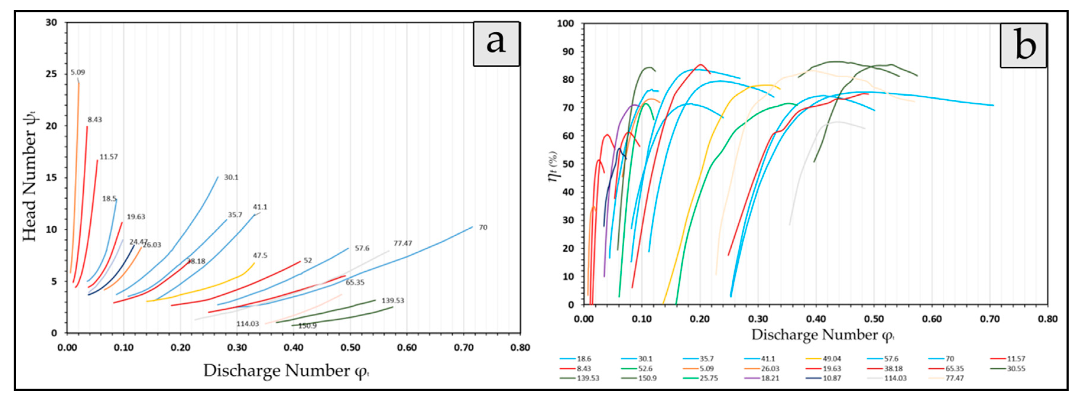
Water 12 01818 g002
Figure 3. (a) Non-dimensional numbers of discharge and head as a function of the specific speed. (b) Non-dimensional number of discharges as a function of the specific speed.
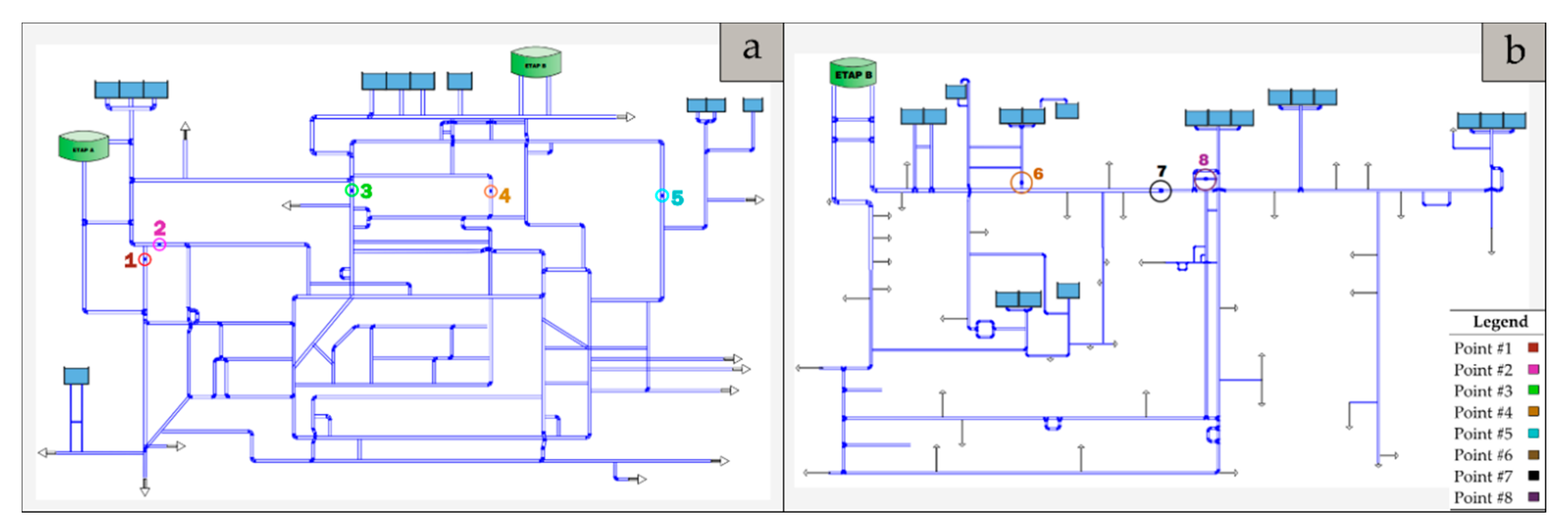
Water 12 01818 g003
Figure 4. High-pressure water distribution system scheme from the VMS: (a) Points 1–5. (b) Points 6–8. Note. ETAPB is the connection point between schemes.
Water 12 01818 g004
Figure 5. (a) Registered flow variability for each study point. (b) Registered dissipated head variability for each study point.
Water 12 01818 g005
Figure 6. Energy distribution comparison for each point.
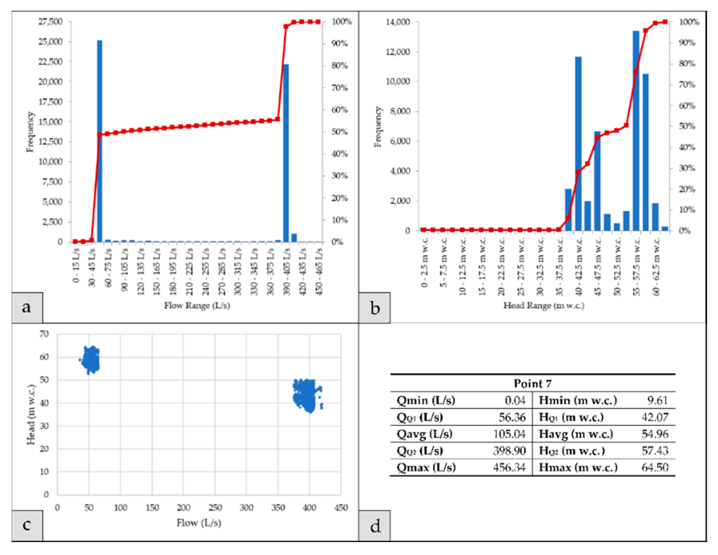
Water 12 01818 g006
Figure 7. (a) Flow chart, 15 L/s intervals, from point #7. (b) Flow chart, 15 L/s intervals, from point #7. (c) Scatter plot for Q vs. H from point #7. (d) Registered values variability for point #7.
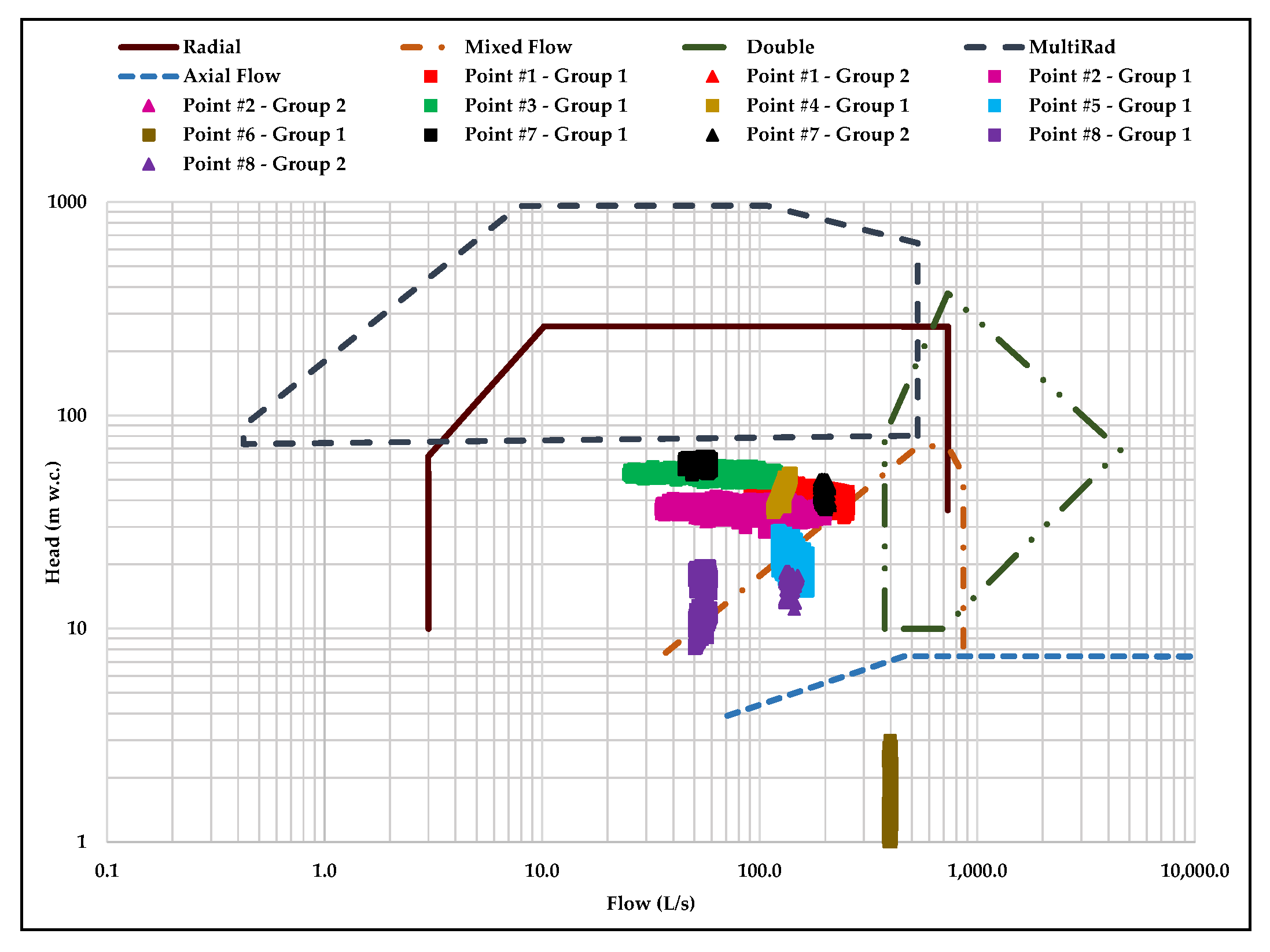
Water 12 01818 g007
Figure 8. Classification for each PAT as a function of the representative operational point for each analyzed case.
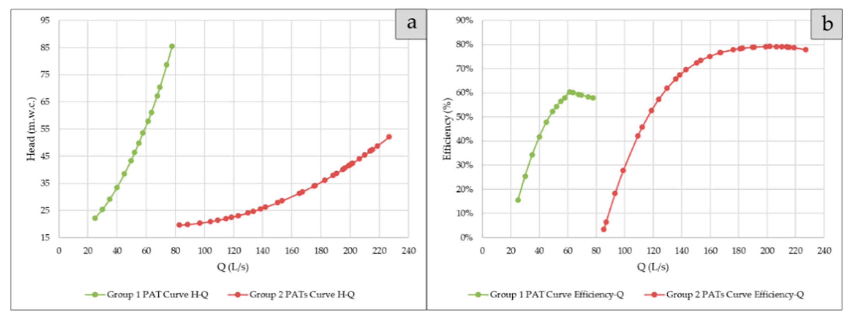
Water 12 01818 g008
Figure 9. (a) Curve Q-H for the selected PATs from group 2. (b) Curve Q-efficiency for the selected pumps from group 2.
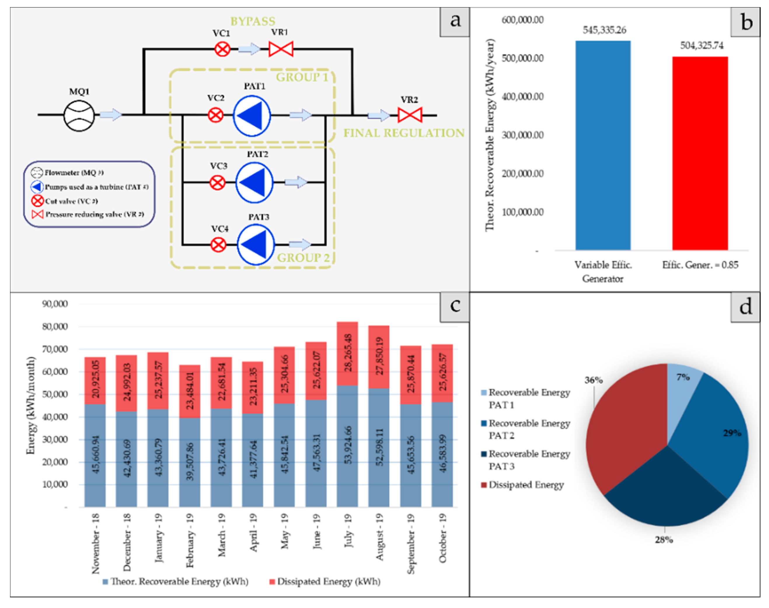
Water 12 01818 g009
Figure 10. (a) PATs installation scheme for point #7. (b) Theoretical recovery energy for each scenario. (c) Energy recovered by PAT. (d) Energy distribution by month.
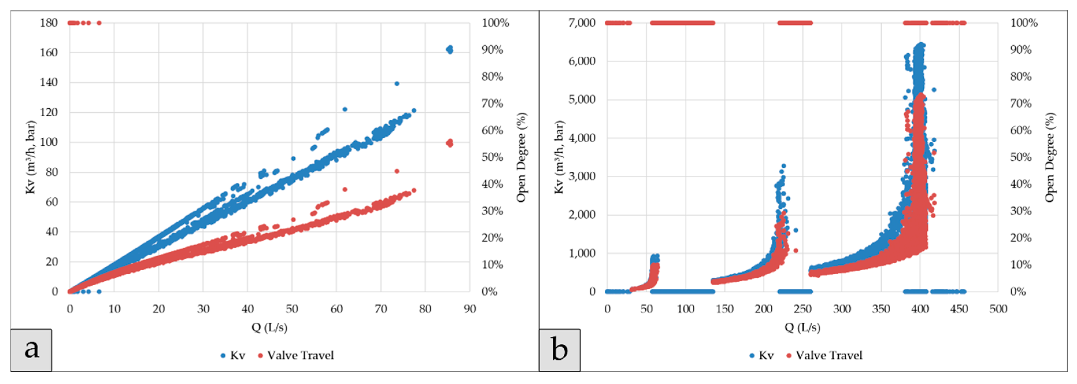
Water 12 01818 g010
Figure 11. (a) Kv and valve travel for each registered flow for the bypass valve. (b) Kv and open degree for each registered flow for the bypass valve.
Water 12 01818 g011
Table 1. Advantages and disadvantages of different pressure management methods.
MethodAdvantagesDisadvantagesReferences
Pressure reducing valves (PRVs)
  • Cheapest initial investment.
  • Decreases water leaks in the network.
  • Manages the pressure downstream of the valve.
  • Relatively simple design and operation.
  • The energy dissipates but is not recovered.
  • Flawed use if the energy is introduced into the system.
[4,5]
Pressure management zones (PMZs)
  • Ease of pressure management due to isolation of topographically different zones.
  • Better use of energy introduced into the system.
  • Higher construction investment.
  • Depends on the topography.
  • Need to install PRVs to regulate remaining overpressure.
[6,7,8]
Pumps used as turbines (PATs)
  • Energy recovery.
  • Decreases water leaks in the network.
  • Manages the pressure downstream of the PAT.
  • Higher investment.
  • Relatively complex design and operation.
  • Need to install PRVs to regulate remaining overpressure.
[9,10,11,12]
Table 2. Data recovered from an analyzed point.
Time (∆t = 10 min)Q (L/s) P u   ( m   w . c . ) P d   ( m   w . c . )
07-11-18 00:00160.9878.2332.95
07-11-18 00:10160.0878.2832.36
07-11-18 00:20159.8678.2832.42
07-11-18 00:30137.1478.3832.18
07-11-18 00:40115.0478.5032.27
07-11-18 00:50104.9478.4431.63
07-11-18 01:0095.4078.7332.25
07-11-18 01:1081.6478.7231.60
07-11-18 01:2072.9579.0232.25
07-11-18 01:3067.2279.0532.10
07-11-18 01:4063.6679.0731.69
07-11-18 01:5074.8678.9631.89
07-11-18 02:0076.9678.8231.57
07-11-18 02:1076.9778.8531.51
Minimum Value0.2926.3328.66
Maximum Value768.3679.6775.37
Mean Value342.9076.2333.90
Standard Deviation147.041.901.78
Table 3. Calculation expression for the different types of energy in a water distribution system.
EnergyCalculation Expression
Total energy (ET) E T ( kWh ) = 9.81 3600   Q i   ( z 0   z i )   Δ t (1)
Friction energy (EFR) E FRi ( kWh ) = 9.81 3600   Q i   ( z 0 ( z i + P i ) )   Δ t (2)
Theoretical energy necessary (ETN) E TNi ( kWh ) = 9.81 3600   Q i   P min i   Δ t (3)
Energy required for consumption (ERI) E RIi ( kWh ) = 9.81 3600   Q i   P min C   Δ t (4)
Theoretical available energy (ETA) E TAi ( kWh ) = 9.81 3600   Q i   ( P i   P min C )   Δ t (5)
Theoretical recoverable energy (ETR) E TRi ( kWh ) = 9.81 3600   Q i   H i   Δ t (6)
Theoretical unrecoverable energy (ENTR) E NTRi ( kWh ) =   E TAi E TRi (7)
Table 4. Empirical relationship to define the best efficiency point of a machine as a function of the specific speed proposed by [20]. In Table 4, the variable η B E P , P is the best efficiency obtained from the machine working as a pump.
CoefficientEmpiric Expression
n S T 0.844564 × n S P
β Q 1 0.825861 × η B E P , P
β H 1.2337 η B E P , P
β η 0.250976 × ln ( n S P )
n S P 1.17619 × n S T
β Q 1 0.210551 × ln ( n S T )
β H 1 0.186314 × ln ( n S T )
Table 5. Proposed empirical equations to predict conversion coefficients.
Author β Q   β H   β η  
Stephanoff
[22]
1 η B E P , P 1 η B E P , P 1
Mc. Claskey
[23]
1 η B E P , P 1 η B E P , P 1
Alatorre-Frenk
[24]
0.85 η B E P , P 5 + 0.385 2 η B E P , P 9.5 + 0.205 1 0.85 η B E P , P 5 + 0.385 1 0.03 η B E P , P
Sharma-Williams
[25]
1 η B E P , P 0.8 1 η B E P , P 1.2 1
Yang et al.
[26]
1.2 η B E P , P 0.55 1.2 η B E P , P 1.1
Hancock
[27]
1 η B E P , P 1 η B E P , P
Barbarelli
[28]
0.00029 n S P 2 0.02771 n S P + 2.01648 3 · 10 5 n S P 3 + 4.4 · 10 3 n S P 2 0.20882 n S P + 4.64293
Grover
[29]
2.379 0.0264 n S T 2.693 0.0229 n S T
Hergt
[30]
1.3 1.6 n S T 5 1.3 6 n S T 3
Table 6. Proposed sustainability indicators.
AbbreviationUnitsIndicatorCalculation
IEDDimensionlessEnergy dissipation I E D = E F R i   ( i n c l u d i n g   v a l v e s ) E I N P U T
IAEkWh/yearAnnual consumed energySum of the total active energy consumed in the network
IEFWkWh/m3Consumed energy per unit volumeRatio between the active energy consumed and the total volume of water introduced in the system
IEC€/m3Energy cost per unit volume introducedRatio between energy cost and the total volume of water introduced in the system
IERkWh/yearEnergy recoveredSum of total energy recovered in the network
ERP%Recoverable energy percentageRecoverable energy percentage used of the total energy consumed in the system
IAAEkWh/yearAbsolute annual consumed energySum of the total active energy consumed in the network subtracted by the sum of the total energy recovered in the network
IAEFWkWh/m3Absolute consumed energy per unit volumeRatio between IAAE and the total volume of water introduced in the network
Table 7. Annual energy distribution from point #7.
Annual Energy Distribution
Total Energy (kWh)1,477,364.03Percentage (%)
Theoretical Recoverable Energy (kWh)847,301.4757.35%
Theoretical Unrecoverable Energy (kWh)630,062.5642.65%
Table 8. Highlights from energy balance at point #7 for each scenario.
Energy Production with PATs Installed
Categoryη = 100%η = 60%Units
Max Theoretical Rec. Power199.57119.74kW
Avg. Theoretical Rec. Power28.0357.87kW
Theoretical Rec. Energy (Annual)847,301.47508,380.88kwh/year
Avg. Theoretical Rec. Energy (Monthly)70,608.4642,365.07kwh/month
Min Theoretical Rec. Energy (Monthly)62,991.8737,795.12kwh/February
Max Theoretical Rec. Energy (Monthly)82,190.1549,314.09kwh/July
Avg. Theoretical Rec. Energy (Daily)2315.031389.02kwh/day
Avg. Theoretical Rec. Energy (Hourly)96.4657.88kwh/h
Table 9. Operational point for each PAT at every study case.
Operational for each Analyzed PointAssumed n (rpm)1450
Analyzed PointPAT GroupPATs in GroupFlow (L/s)Head (m w.c.)nST (m, kW)
Point #112 (Parallel)210.0040.5041.39
21117.5046.5027.91
Point #21 (Parallel)1125.0036.5034.52
1175.0036.5040.85
Point #31 (Parallel)380.0051.7521.26
Point #411132.5047.5029.17
Point #51 (Parallel)3141.6724.0050.33
Point #6Not enough data to select a pump
Point #71157.0056.0016.91
22 (Parallel)200.0041.5039.66
Point #812 (Parallel)57.0010.5059.35
21143.5016.0068.66
Table 10. Initial data for conversion from point #7.
Initial Data—Point #7
CategoryGroup 1Group 2Units
QBEPt57.00 200.00 L/s
HBEPt56.00 41.50 m w.c.
nt1450.00 1450.00 rpm
nst16.91 39.66 m, kW
Table 11. Data conversion from turbine mode to pump mode (point #7).
Data Conversion from Turbine Mode to Pump Mode
AuthorsGroup 1Group 2
βQβHQBEP, p (L/s)HBEP, p (m w.c.)βQβHQBEP, p (L/s)HBEP, p (m w.c.)
Pérez-Sánchez et al.1.681.9033.9429.511.291.46154.9828.46
Grover1.932.3129.4924.291.331.78150.1523.25
Hergt1.170.8748.9064.471.251.14159.5136.52
Table 12. Selected pumps and best efficiency point data for each group (point #7).
Selected Pump for Each Group
Group 1Group 2
ModelCPH 100-375ModelNK 150-315
QBEP P37.42 L/sQBEP P146.85 L/s
HBEP P30.00 m w.c.HBEP P27.40 m w.c.
ηBEP P0.69 -ηBEP P0.82 -
nP1450 rpmnP1,450 rpm
nsp21.88 m, kWnsp46.40 m, kW
Table 13. Conversion coefficients from pump mode to turbine mode for each group of point #7.
Conversion Coefficient (from Pump Mode to Turbine Mode)
Group 1Group 2
ModelCPH 100–375ModelNK 150–315
AuthorsβQβHβηβQβHβη
Pérez-Sánchez1.461.790.881.341.510.98
Stephanoff1.21.4511.11.221
Mc. Claskey1.451.4511.221.221
Alatorre-Frenk1.961.930.961.381.430.96
Hancock1.451.45N/A1.221.22N/A
Barbelli1.551.87N/A1.361.43N/A
Yang et al.1.471.8N/A1.341.49N/A
Sharma-Williams1.351.5611.171.271
Table 14. Pump mode operation point estimation for each group of point #7.
Pump Mode Operational Point Estimation
Group 1Group 2
ModelCPH 100-375ModelNK 150-315
AuthorsQBEP T (L/s)HBEP T (m w.c.)ηBEP TnSTCQBEP T (L/s)HBEP T (m w.c.)ηBEP TnSTC
Pérez-Sánchez54.5553.640.6117.090.14196.4841.270.839.470.07
Stephanoff45.0543.480.6918.180.73162.2733.460.8241.990.64
Mc. Claskey54.2343.480.6919.940.99179.333.460.8244.140.67
Alatorre-Frenk73.4457.920.6618.721.38203.0139.240.7941.670.35
Hancock54.2343.48N/A19.940.99179.333.46N/A44.140.67
Barbelli57.9655.98N/A17.060.0919939.18N/A41.310.27
Yang et al.55.0754.15N/A17.050.11196.6740.96N/A39.720.05
Sharma-Williams50.3546.830.6918.180.52172.2834.820.8241.990.51
Table 15. Best efficiency point (BEP) (pump and turbine mode) for the selected pumps from each point.
Analyzed PointPAT GroupPump SelectedBest Efficiency Point for Selected PumpsBest Efficiency Point (Turbine Mode)
Q (L/s)H (m w.c.)ηPnSP (m, kW)Flow (L/s)Head (m w.c.)ηTnST (m, kW)C
Point #11TP 200-320/4154.627.80.8447.2204.440.80.8340.60.17
2GNI 150-40/7590.034.30.8330.7119.651.00.7726.30.44
Point #21GNI 150-32/4085.524.00.8139.1115.036.60.7833.10.43
RNI 200-32127.522.50.850.1173.134.90.7942.00.19
Point #31GNI 125-32/4056.231.90.7825.677.150.50.721.30.12
Point #41GNI 150-32/60102.133.10.8533.6134.148.00.829.10.04
Point #51CPH 150-290103.015.470.8359.7137.323.10.8450.90.11
Point #6Not enough data to select a pump
Point #71CPH 100-37537.430.00.6921.954.653.60.6117.10.14
2NK 150-315146.927.40.8246.4196.541.30.839.50.07
Point #81NB/NK 125-200/196-17253.07.60.7773.273.312.20.860.30.98
2NB/NK 150-250104.210.90.7478.3146.318.00.7863.40.58
Table 16. Defining variables for the empirical curves from the selected PATs.
Selected PATs for Each Group
Group 1Group 2
ModelCPH 100-375ModelNK 150-315
QBEP T54.55 L/sQBEP T196.48 L/s
HBEP T53.64 m w.c.HBEP T41.27 m w.c.
ηBEP T0.61 ηBEP T0.80
nT1450.00 rpmnT1450.00 rpm
nST17.09 m, kWnST39.47 m, kW
D325.00 mmD310.00 mm
φ0.07 (m3/s, rps)φ0.27 (m3/s, rps)
ψ8.53 (m/s², rps²)ψ7.21 (m/s², rps²)
Table 17. Selected valves for the system.
By-PassFinal Regulation
Model700-ES700/700-EN
Connection TypeY-PatternG-Pattern
Disc TypeFlat DiscFlat Disc
DN (mm)125600
K V (m3/h, 1 bar)2157300
Table 18. Sustainability indicators for point #7 [3].
BeforeAfterChange
IED0.580.21−64.16%
IAE (kWh/year)1,477,364.031,477,364.03
IEFW (kWh/m3)4.064.06
IEC (€/m3)0.0360.023−35.01%
IAAE (kWh/year)1,477,364.03932,028.77−36.91%
IAEFW (kWh/m3)4.062.56−36.91%
IER (kWh/year) 545,335.26+545,335.26
ERP (%) 36.91%+36.91%

