A Modified ABCD Model with Temperature-Dependent Parameters for Cold Regions: Application to Reconstruct the Changing Runoff in the Headwater Catchment of the Golmud River, China

Abstract

The runoff changes due to global warming in hydrological basins in the Qinghai–Tibetan Plateau (QTP) have received worldwide attention. The headwater catchment of the Golmud River, located in the northern QTP, is the main source of water resources for the Golmud city in an arid region but has been poorly known for the hydroclimatological behaviors. In this study, a widely-used hydrological model, the ABCD model (Thomas, H.A., Washington, DC, USA), is modified by incorporating temperature-dependent hydrological processes and groundwater evapotranspiration in cold regions with a few additional parameters. The new model is used to reconstruct the monthly runoff in the past decades for the headwater catchment of the Golmud River and performs better than other comparable models. As indicated, the annual snowmelt runoff increased with the increasing air temperature and became more concentrated in April than in May. The frozen soil degradation could increase the hydraulic conductivity of soils and lead to a rise in cold season runoff. The groundwater level in the Golmud city was positively correlated to the annual runoff in the headwater catchment of the Golmud River, indicating that an increase of the groundwater level could be triggered by the rising trend in the streamflow of the Golmud River. This study suggests a useful hydrological model for the groundwater management in the Golmud city.

1. Introduction

Catchments in mountains generally role as headwater region for adjacent lowlands, providing variable water resources with the changing runoff that have great impacts on humanity and ecosystems in the middle and lower reaches area [1]. Most of the large mountains in the world are cold with a local climate that is sensitive to the rapid global warming in the last decades. Climate change caused by global warming may significantly alter the hydrological processes in headwater catchments, leading to a remarkable shift in the water balance, available water resources and extremes events (floods and droughts) [2,3,4]. Therefore, it is a great challenge to assess or predict the change in the runoff of headwater catchments for better managements of water use and ecosystem protections.

The Qinghai–Tibetan Plateau (QTP) roles as the water tower of Asia, which is the source area of many large Asian rivers, such as the Yellow River, Yangtze River, and Brahmaputra River, providing water resources for more than 1.4 billion of people [5]. The QTP has experienced significant warming during recent decades [6,7,8,9,10], and precipitation in the QTP has also experienced evident changes [11]. The impact of climate change is considered one of the major threats to the water resources in the QTP [12]. Landscape changes in the QTP, e.g., changes in the cryosphere and vegetation, have been also reported [13,14]. Therefore, the change in runoff with the influence of climate and landscape changes has gradually become a hot topic in the research of regional hydrology in the QTP [15,16,17,18,19,20]. However, it is still a poor known factor with uncertainties for assessments on the hydrological changes in the headwater catchments in the QTP due to limited observations [21,22,23,24].

River discharge is an essential hydrological variable to analyze runoff changes in the headwater catchment. With large portions of ungauged areas, long-term high-resolution monitoring of river discharge was absent in the QTP for many rivers. There has been a growing interest in retrieving river discharge from remote sensing via altimeters [25] and spectral bands [26] over inland water bodies. However, these techniques are mainly developed for large rivers and are not applicable to many high-mountain QTP rivers, which feature complex topography and relatively narrow channels. Recently, some studies developed data-driven models to reconstruct river discharge based on the machine learning method [27,28]. However, data-driven models need huge amount of training data, which are usually not available in the QTP due to scarce observations.

Compared with the method based on remote sensing, hydrological model simulation, driven by observed atmosphere forcing data including precipitation, air temperature, and potential evaporation may provide an accurate and flexible tool to reconstruct the long-term runoff series. Several existing studies incorporated complex snow and frozen soil models with distributed hydrological models for cold regions and illustrated the improvement of model performance for runoff simulation [29,30,31]. However, these models need high resolution data, and are difficult to be applied in basins with extremely limited observations. Liu et al. [32] simulated snowmelt and monthly runoff of six major rivers including the Qaidam Basin from 1980 to 2013 using the Soil and Water Assessment Tool (SWAT) model (United States Department of Agriculture, Washington, DC, USA). However, due to the lack of observations, the runoff was not validated in most sub-basins including the headwater catchment of the Golmud River. Therefore, due to the scarce observations of complex environmental information, it is not an efficient way to use distributed hydrological models in estimating runoff or predicting long-term hydrologic responses to the climate change in most basins on the QTP, so that conceptual hydrological models were recommended [23]. In some studies, statistical methods were used to generate the rainfall scenarios [33,34] for climate impact analysis, and in several other studies, the Budyko framework [35] was adopted. For example, Wu et al. [36] investigated the relationship between the change in the permafrost and the parameter of the Budyko model for source regions of the Yellow River. Wang et al. [37] also applied the Budyko model in a study of source regions of the Yellow River and they argued that frozen ground degradation could reduce runoff by increasing groundwater storage. These studies focused on the inter-annual change in streamflow because the Budyko hypothesis is limited to the mean annual water balance. This indicates that it cannot be applied for simulating and reconstructing monthly runoff. A few of the existing studies attempted to simulate and analyze the changes in monthly or daily streamflow of rivers in the QTP by using complicated distributed hydrological models [29,38,39]. However, as previously highlighted, the use of process-based distributed hydrological models in the QTP region is a challenge because of significant limitation in observations and large requirement of computational resources. It is promising to develop models that are minimally parameterized, efficient, and accurate [40].

Unlike the Budyko framework, the ABCD model developed by Thomas [41] was a conceptual hydrological model that can be used for the monthly or annual water balance. It only has four parameters but clearly incorporates major hydrological processes and has been widely adopted in hydrological studies. Alley [42] demonstrated that the ABCD model performs well in comparison with other conceptual models for the monthly runoff simulation. Zhao et al. [43] argued that the Budyko-type model at the annual scale and the SCS model at the rainfall-event scale could be considered as the special extensions of the monthly ABCD model. This result illustrated the rigorous physical basis of the ABCD model. By using the ABCD model, Sankarasubramanian and Vogel [44] examined the water balance of 1337 basins in the United States to explain the annual hydroclimatology of the United States in the Budyko space. Wang and Zhou [45] modified the ABCD model by considering groundwater evaporation and investigated the runoff changes in the Erdos plateau in Northwest China where the climate is arid to semiarid. Han and Wang [46] well predicted the hydrological response to potential extreme climate changes in the NLRB basin in the USA using the ABCD model. Therefore, the ABCD model may be considered as an efficient tool for reconstructing the runoff in poorly observed rivers on the QTP. Nevertheless, it is uncertain that the ABCD model can be efficiently used for catchments in cold regions with permafrost because frozen soils and snowmelt were not considered in the model. An attempt was made by Martinez and Gupta [47] who developed an augmented ABCD-snow model with temperature-dependent components. This model introduced three parameters for the snow accumulation and melt processes but the other parameters in the ABCD model were still assumed to be independent on the air temperature.

This study focuses on further improvement of the ABCD model for catchments in cold regions. We suggest several new formulas to handle the change in control parameters of the ABCD model with the change in the air temperature. A few additional parameters are introduced. This modified model incorporates the effect of temperature-dependent frozen soils on the hydrological processes in cold regions. We use both of the new model and the original ABCD model to simulate and restore monthly runoff data in the headwater catchment of the Golmud River which is located in the northern QTP. As indicated from comparison between results of different models, the modified model performs much better. Based on the calibrated model, we reconstructed the monthly river discharge in the headwater catchment of the Golmud River and investigate the long-term changes in the streamflow in the period from 1975 to 2015. At last, we analyzed the relationship between the runoff of the headwater catchment of the Golmud River and the groundwater level in the Golmud city.

2. Study Area and Data

2.1. The Study Area

The study area (Figure 1) is the headwater catchment of the Golmud River that originates from the Naijin River and Xueshui River in the Kunlun Mountains [48], northern QTP. It has an area of 18,675 km², mainly covered by sparse grassland and barren land [49]. The elevation of ground surface ranges from 3427 m to 5659 m. The mean annual precipitation and air temperature are 260 mm and 1.83 °C, respectively. In most of the mountain area, the mean air temperature is less than zero, forming permafrost, glacier, and snowpacks. The mean annual river discharge at the outlet of headwater catchment of the Golmud River is 26 m³/s. In average, the Naijin River and Xueshui River contributes 78% and 22%, respectively, to the total streamflow in the Golmud River. This is the only surface water resource of the Golmud city where the mean annual precipitation is less than 50 mm under an extremely arid climate condition. The Golmud River is an endorheic river in the Qaidam Basin, which terminates at the Dabson Lake, a hypersaline lake.

The leakage of water from the Golmud River is the major recharge of groundwater in the area of the Golmud city. This recharge highly depends on the runoff of the headwater catchment of the Golmud River. As a consequence, the groundwater level in the Golmud city is subject to the streamflow in the river. Due to changes in streamflow, the depth to subsurface water table in Golmud City has experienced large oscillations in the past 40 years. In 1981, 1983, and 2010, significant rise of the groundwater level caused serious disasters in the city area such as house collapses and grassland immersion [50,51]. Previous studies on this kind of groundwater disasters mainly focused on the inter-annual change in groundwater level [52,53], but it has been highlighted that groundwater in this area is closely related to surface water [54]. However, one of the difficulties in the management of the Golmud groundwater is the lack of understanding of long-term runoff changes in the headwater catchment of the Golmud River, where frozen soils exist and streamflow is sensitive to climate change in the QTP.

2.2. Data and Treatment

Several datasets were used in this study to prepare the input of the hydrological models, including the distributed precipitation (P), air temperature (T), and potential evaporation (E₀). As shown in Figure 1, there was no national meteorological station in the headwater catchment of the Golmud River, although some meteorological stations exist around the study area. To estimate the basin-averaged monthly precipitation, the recently released global precipitation product TERRACLIMATE data [55] was used, which has a spatial resolution of 4 km. Among the nearby national meteorological stations (Figure 1), Golmud (with the lowest altitude) and Qumarleb (with the highest altitude), were selected to examine the accuracy of the TERRACLIMATE precipitation data. The observed mean monthly precipitation during 1965–2015 at the two meteorological stations are shown in Figure 2 and are compared with the TERRACLIMATE data at pixel elements where the stations located in. It indicates that the TERRACLIMATE data agreed well with the observed precipitation. This agreement illustrates that the TERRACLIMATE precipitation data are reliable in the study area and can be used to estimate the average precipitation from this distributed data.

The distributed potential evaporation and air temperature were interpolated with distance weighting method from six national meteorological stations around the study area (Figure 1). The correlation between the air temperature and the elevation [50] was incorporated in generating the distributed air temperature. The potential evaporation was calculated as the pan evaporation (E_pan) observed from a standard pan (601 mm in diameter) at each meteorological station multiplying an empirical coefficient [56]. Daily T, P and E_pan at the meteorological stations were obtained from the dataset released by the China Meteorological Data Service Center (http://data.cma.cn). These data were then used to estimate the monthly and annual T, P, and E₀. A brief summary of the meteorological data was provided in

Table 1. Background data of meteorological stations (period 1965–2015).

Station	Xiaozaohuo	Golmud	Nuomuhong	Wudaoliang	Qumarleb	Madol
Altitude (m)	2767.0	2807.6	2790.4	4612.2	4175.0	4272.3
Mean annual P (mm)	28.9	43.9	47.8	293.3	416.3	324.2
Mean annual T (°C)	3.9	5.5	5.1	−5.1	−1.9	−3.5
Mean annual E0 (mm)	1570.0	1538.1	1351.9	795.6	770.6	881.6
Trend in P (mm/yr)	+0.13	+0.16	+0.48	+2.22	+1.23	+1.41
Trend in T (°/a)	+0.06	+0.05	+0.04	+0.03	+0.04	+0.04
Trend in E0 (mm/yr)	+1.22	−9.14	−7.42	−1.33	+3.13	+1.81

. The monthly and annual T and E₀ data at these meteorological stations were interpolated to produce 4-km resolution raster data in the study area.

Applying the raster data of P extracted from TERRACLIMATE and the raster data of T and E₀ interpolated from the meteorological stations, the basin-average monthly and annual T, P, and E₀ were obtained for the study catchment. Figure 3 shows the annual data between 1965 and 2015 at the basin-scale. As exhibited, there were increasing trends of P and T in the period 1965–2015 with different fluctuations. The trend of E₀ was negative in this period and the fluctuation seemed to be also in contrast to that of T. This decreasing trend in E₀ is consistent with the decreasing trend in E_pan indicated by meteorological observations in the past 50 years around China [57,58]. Existing analyses found that this negative trend in E_pan was linked with the decreasing wind speed and solar radiation as well as the increasing relative humidity [57,58], even though the increasing air temperature was expected to be an positive factor for the evaporation process. Indeed, such a “paradox” did not only exist in China but also was found to be a global phenomenon, which has been interpreted as a result of significant decreases in sunlight due to increased cloud coverage and aerosol concentration [59]. Linear slope in trends of T, P, and E₀ at different meteorological stations are listed in Table 1. It is indicated that the slope of T was relatively uniform for different places but the slope of P and E₀ show significant spatial variance. In particular, the trend of E₀ was positive in some places, not always negative. These differences imply the complexity of the climate change in the QTP.

Streamflow in the Golmud River were observed at two different hydrological stations shown in Figure 4a that operated in different periods. Groundwater levels in the region near the Golmud city were monitored in observation wells G1–G4 (Figure 4a), with available data from 1990 to 2012 as shown in Figure 4b. The regime of groundwater levels was significantly influenced by the streamflow in the Golmud River observed at hydrological stations. The first hydrological station, W-III, was established before 1965 at the outlet of the headwater catchment of the Golmud River but destroyed by a heavy flood in 1990. The second hydrological station, W-IV, was established in 1990 at a lower reach to replace the W-III station, where the streamflow changed since 1990 as shown in Figure 4c. Several reservoirs have been constructed in the river between W-III and W-IV since 1977. A significant leakage of water from the reservoirs and riverbeds exists between W-III and W-IV because the groundwater level over there is lower than the surface water level. Thus, the streamflow at W-IV does not represent the actual runoff in the study catchment. However, the annual streamflow during 1990–2015 at W-III has been estimated from the W-IV data using a restoration method in a previous study [54]. The combined annual streamflow data at W-III are shown in Figure 4d. As indicated, the annual runoff shows a significant fluctuation, partly following the variations of the local precipitation. The relationship between the annual streamflow and groundwater level is discussed in Section 4.5.

3. Methodology

3.1. ABCD Model

The ABCD model divides the whole catchment water storage into soil water and groundwater [41], as that shown in Figure 5a. The rainfall (P) is partitioned into the evapotranspiration (E), the surface runoff (D), and the change in soil water storage. A delayed infiltration from the soil water recharges the groundwater. The total runoff is a combination of the surface runoff and the base flow that released from groundwater.

For a monthly simulation, the change in soil water storage in the ith month is calculated as follows:

$$S_i-S_{i-1}=P_i-E_i-R_i-D_i$$

(1)

where $S_{i-1}$ and $S_i$ are, respectively, the effective soil water storages at the end of (i − 1)th and ith month, $P_i,E_i,R_i\mathrm{and}{D}_i$. are the precipitation, actual evapotranspiration, groundwater recharge and surface runoff in the ith month, respectively. The change in groundwater storage is calculated as follows:

$$G_i-G_{i-1}=R_i-F_i$$

(2)

where $G_i\mathrm{and}{G}_{i-1}$ are, respectively, the effective groundwater storages at the at the end of (i − 1)th and ith month, $F_i$ is the base flow in the ith month. The ABCD model estimates $R_i$,$G_i,$and $F_i$ as follows:

$$R_i=c{W}_i-Y_i$$

(3)

$$D_i=(1-c)(W_i-Y_i)$$

(4)

$$F_i=d{G}_i$$

(5)

where $c$ and $d$ are two dimensionless parameters for the monthly simulation, whereas $W_i$ and $Y_i$are two state variables defined, respectively, as follows:

$$W_i=P_i+S_{i-1}$$

(6)

$$Y_i=E_i+S_i.$$

(7)

A nonlinear relationship between $Y_i$and $W_i$ was proposed [42]:

$$Y_i(W_i)=\frac{W_i+b}{2a}-{\left[{\left(\frac{W_i+b}{2a}\right)}^2-\frac{W_{i}b}{a}\right]}^{0.5}$$

(8)

where a (dimensionless) and b (mm) are two parameters. The values of S_i and G_i are finally estimated as:

$$S_i=Y_{i}exp(-\frac{E_{0i}}{b})$$

(9)

$$G_i=\frac{\left[c\left(W_i-Y_i\right)+G_{i-1}\right]}{1+d}$$

(10)

where $E_{0i}$ is the potential evaporation in the ith month.

In the ABCD model, the summation of the surface runoff, D_i, and the base flow, F_i, yields the total runoff,$Q_i$, which can be expressed as follows:

$$Q_i=(1-c)(W_i-Y_i)+d{G}_i$$

(11)

3.2. Modified ABCD Model for Cold Regions (ABCD-CR)

The first essential condition that should be considered in cold regions is the existing of frozen soils, which highly depends on the air temperature. In general, frozen soils are low-permeability materials that can decrease the effective hydraulic conductivity of shallow soils and aquifers for the subsurface flow. Therefore, development of shallow frozen soils when the air temperature dropped below the freezing point could reduce both of groundwater recharge and discharge [60]. This mechanism was not considered in the ABCD model but the parameters c and d were related to groundwater recharge and discharge. We suggest a modification of c and d from constants to temperature-dependent parameters as follows:

$$c=\{\begin{array}{c}{c}_0{e}^{\alpha T_i},T_i\le 0\\ c_0,T_i>0\end{array},d=\{\begin{array}{c}{d}_0{e}^{\alpha T_i},T_i\le 0\\ d_0,T_i>0\end{array}$$

(12)

where $\alpha$ is an additional parameter (1/°C) representing the influence of negative air temperature, $T_i$ is the basin-average monthly mean air temperature, c₀ and d₀ are normal values of c and d when the air temperature is positive.

Another condition that should be considered in cold regions is the snow cover (possibly overlying glaciers). Snowmelt water (possibly including the release of glaciers) could be an additional supply to the soil water in non-frozen seasons, particularly in April and May. This was also ignored in the ABCD model. To modify the model, we divide the total precipitation, $P_i^{^}$, into the rainfall, $P_i^{\prime }$, and the snowfall, $P_i^{*}$, as follows:

$$P_i^{\prime }=\{\begin{array}{c}0,T_i\le 0℃\\ P_i^{^},T_i>0℃\end{array},P_i^{*}=\{\begin{array}{c}{P}_i^{\prime },T_i\le 0\\ 0,T_i>0\end{array}.$$

(13)

Here we did not follow the snow model supposed by Martinez and Gupta [47] who introduced two temperature thresholds and required daily minimum temperature data for input. The practicability of Equation (13) is higher because it does not include additional parameters and only require the average monthly mean air temperature. The snowfall increases the solid water storage in the snow cover and/or glaciers, $S_i^{*}$, as:

$$S_i^{*}=S_{i-1}^{*}+P_i^{*},\mathrm{for}{T}_i<0.$$

(14)

When $T_i$ is higher than 0 °C, it is considered that a basin-scale snowmelt water depth (possibly mixed with melting glaciers), $D_i^{*}$, will comes into being as follows [61]:

$$D_i^{*}=\beta T_i{S}_{i-1}^{*},\mathrm{for}{T}_i>0$$

(15)

where β is also an additional parameter (1/°C). Equation (15) is different from the snowmelt formula proposed by Martinez and Gupta [47], who assumed that the released runoff from the snowmelt is independent on temperature when the air temperature is higher than the “rain” threshold. Their assumption is not reasonable because the snowmelt rate is highly dependent on the air temperature. In the frozen season with $T_i$< 0, we assume that $D_i^{*}$= 0. A positive D* will cause a decrease in S*:

$$S_i^{*}=S_{i-1}^{*}-D_i^{*}=\left(1-\beta T_i\right)S_{i-1}^{*},\mathrm{for}{T}_i>0$$

(16)

Note that $D_i^{*}$ should be restricted to $S_{i-1}^{*}$when the result of Equation (15) is higher than $S_{i-1}^{*}$. In this study we include the smelt water in the equivalent precipitation $P_i$(The role of $P_i$ is the same of that in the ABCD model.) on the land surface, as follows:

$$P_i=P_i^{\prime }+D_i^{*}$$

(17)

In addition to the previous modification, we introduce the groundwater evapotranspiration in the model. Wang et al. [45] highlighted that the groundwater evapotranspiration in zones with a small depth to water table could significantly influence the catchment water balance. In cold regions, shallow groundwater with relatively high temperature maintains unfrozen soils and can directly contribute to the land surface evapotranspiration. The groundwater evapotranspiration occurs in a small part of the catchment and roles as an additional loss of water from the normal soil water evapotranspiration, which depends on the depth to water table with a complicate process. To simplify the simulation, in this study we assume that the groundwater evapotranspiration at the basin scale,$E_i^{*}$, is proportional to both of the groundwater storage, $G_i$, and the potential evaporation, $E_{0i}$, in excess of the soil water evapotranspiration,$E_i$, as follows:

$$E_i^{*}=\frac{G_i}{G_{max}}\left(E_{0i}-E_i\right)$$

(18)

where $G_{max}$ is the potential maximum groundwater storage (L).

The modifications on the frozen soils, snow cover and groundwater evapotranspiration are incorporated into the original ABCD model to develop a new conceptual hydrological model, named ABCD-CR, for catchments in cold regions. The outline of ABCD-CR model is shown in Figure 5b. Equations (3)–(9) in the ABCD model are still applied but includes the temperature-dependent parameters defined in Equation (12). The change in groundwater storage is estimated by:

$$G_i-G_{i-1}=c\left(W_i-Y_i\right)-d{G}_i-E_i^{*}.$$

(19)

Substituting Equation (17) into Equation (18), we have:

$$G_i={\left(1+d+\frac{E_{0i}-E_i}{G_{max}}\right)}^{-1}\left[c\left(W_i-Y_i\right)+G_{i-1}\right].$$

(20)

The total runoff is the summation of the surface runoff, D_i, the base flow, F_i, and the snowmelt runoff,$D_i^{*}$, as follows:

$$Q_i=(1-c)(W_i-Y_i)+d{G}_i+D_i^{*}.$$

(21)

The ABCD-CR model has 7 parameters: a, b, c₀, d₀, G_max, α and β.

3.3. Calibration and Performance Assessment of Models

In this study, not only the ABCD and ABCD-CR models are used. To check the efficiency of considering different processes (frozen soils, snow cover, and groundwater evapotranspiration) in this cold region, we add two models, ABCD-I and ABCD-II, in the comparison. The ABCD-I model is close to the ABCD model, and the only difference is that the ABCD-I model includes the groundwater evapotranspiration. In the ABCD-II model, the temperature-dependent behaviors are incorporated as the same in the ABCD-CR model, but the groundwater evapotranspiration is not considered. It is an equivalent model of ABCD-CR when we specify $G_{max}=\infty$ in Equation (17). After preheating of the models on runoff simulation of the study catchment, we presumed the ranges of parameter values that should be satisfied in the model calibration (

Table 2. Presumed parameter ranges for model calibration and optimal results.

Model	a	b (mm)	c0	d0	α (1/°C)	β (1/°C)	Gmax (103 mm)
ABCD Model	0.8–1.0 (0.96) *	20–160 (98)	0.8–1.0 (0.911)	0.001–0.01 (0.003)	0	/	∞
ABCD-I Model	0.8–1.0 (0.84)	20–160 (45)	0.8–1.0 (0.933)	0.001–0.01 (0.004)	0	/	1–10 (5.2)
ABCD-II Model	0.8–1.0 (0.97)	20–160 (100)	0.8–1.0 (0.923)	0.001–0.01 (0.005)	0.01–0.2 (0.038)	0.01–0.2 (0.053)	∞
ABCD-CR Model	0.8–1.0 (0.86)	20–160 (43)	0.8–1.0 (0.902)	0.001–0.01 (0.004)	0.01–0.2 (0.037)	0.01–0.2 (0.142)	1–10 (5.2)

* Values in () are results of the model calibration.

).

The models were calibrated with the input monthly meteorological data in the period 1982–1985, to produce monthly runoff results matching observation data at the hydrological station W-III in the same period. Modeling performance was assessed using the Nash–Sutcliffe efficiency (NSE) [62]. Better performance is exhibited when NSE is closer to 1. For monthly simulation, the performance would be quite well when NSE > 0.7 and satisfactory when NSE > 0.5. For a test model, the NSE depends on the parameter values and was taken as the objective function in the calibration. The error of the modeling results was also evaluated with the Mean Absolute Relative Error (MARE).

The data in the period 1986–1989 were used to verify the calibrated models. This validation has to be terminated in 1990 when the hydrological station W-III was destroyed. The restored streamflow data [54] from the hydrological station W-IV was not used for the model verification due to uncertainties in estimating the leakage loss between W-III and W-IV. However, the calibrated models can be applied to produce new restored streamflow for the period since 1990 and the result is presented in Section 4.

3.4. Sensitivity Analysis on Runoff to Temperature

In the study area, the change in air temperature is a critical force that triggering changes in climatic and hydrological conditions. To check the unique impact of the change in air temperature on the change in runoff, we perform a special sensitivity analysis using the ABCD-CR model. A hypothesized scenario is used as the baseline for the period 1975–2015 when the air temperature showed a significant increasing trend. This scenario is characterized by a repeat of rising and falling temperature in every year with the same patterns from 1965 to 1974. However, the monthly precipitation and potential evaporation in this scenario are not changed from the actual data. Such a scenario is organized for the ABCD-CR model to produce a baseline of the runoff in the study area and denoted as baseline simulation. The comparison between this baseline simulation and the normal simulation with the actual air temperature is discussed in Section 5.1.

4. Results

4.1. Validation and Calibration Results of the ABCD-CR Model

We calibrated and validated the ABCD-CR model using the observed runoff data, for periods of 1982–1985 and 1986–1989, respectively. The parameters were optimized by maximizing the Nash–Sutcliffe efficiency (NSE) in the calibration period. The time from January 1963 to December 1981 was used as the preheating period to minimize the influence of uncertainties in initial conditions on the model simulation. The length of this period is enough to eliminate the effect of initial conditions on the comparison of different models. The identified parameters of the ABCD-CR model are shown in Table 2. Figure 6 shows the simulated and observed monthly runoff curves at the W-III station for a comparison. The modeling results basically agree with the observation. As shown in

Table 3. Performance of models in calibration and validation periods.

Model	NSE		Error (MARE, %)
	Calibration	Verification	Calibration	Verification
ABCD Model	0.47	0.55	30.07	35.81
ABCD-I Model	0.55	0.59	26.13	28.10
ABCD-II Model	0.63	0.66	19.11	26.32
ABCD-CR	0.72	0.72	17.53	17.25

, the NSE of the ABCD-CR model is greater than 0.7 in both of the calibration and validation periods, indicating that this model performs well. The MARE is less than 20%, also indicating a high accuracy. To check the robustness of the model calibration, an experiment with a longer validation period was also operated. In the experiment, the period 1963–1973 was chosen for model preheating and the period 1974–1977 with mean annual T of 0.99 °C was chosen as the calibration period. A 12 years period from 1978 to 1989 with mean annual T of 1.49 °C, which was warmer than that in the calibration period, was treated as the validation period. Result of the ABCD-CR model in this experiment is shown in Figure S1 in the Supplementary Material, which indicates that the simulated monthly runoff also agrees well with observations at the W-III station. The NSE was 0.70 and 0.69 for the calibration and validation periods, respectively, similar to that of the ABCD-CR model (Table 3) using periods 1982–1985 and 1986–1989 for calibration and validation, respectively. These results illustrate that the calibrated ABCD-CR model is sufficient for long-term runoff simulation in the headwater catchment of Golmud River.

4.2. Comparison among Different Models

We firstly compared the ABCD Model with the ABCD-CR model using the same methods in preheating, calibration, and validation. The calibrated parameters and simulated runoff for the ABCD model are shown in Table 2 and Figure 7a, respectively. The NSE of the ABCD model is less than 0.5 (Table 3) in the calibration period, indicating an unsatisfactory result. Although the NSE is slightly higher than 0.5 in the calibration period, the MARE is quite large (higher than 30%). The ABCD model is not successful in capture the runoff patterns, especially in the summer (Figure 7a). It significantly underestimated the peaks of runoff in summer and overestimated the low flow during the cold season.

The simulated monthly runoff from the ABCD-I model is shown in Figure 7b. The ABCD-I model yields higher NSE values than that of the ABCD model. However, compared with the ABCD-CR model, the ABCD-I model still has lower NSE values and lager MARE (Table 3). The errors are mainly caused by the poor performance in the cold season (October to March). As shown in Figure 7b, the observed runoff decreased from above 4 mm in October to about 2 mm in January when the temperature decreased, while the simulated runoff could not drop so much due to using constant c and d. As shown in Table 2, the b value of the ABCD-I model (less than 50 mm) is quite smaller than the b value in the ABCD model (close to 100 mm) because the limit of Gmax at 5200 mm. It allows the ABCD-I model to capture the high runoff in the summer.

Figure 7c shows the simulated monthly runoff by the ABCD-II model. The NSE of the ABCD-II model is higher than the NSE values of the ABCD and ABCD-I models but still smaller than 0.7 (Table 3). For the runoff in the cold season, the ABCD-II model performs better than the ABCD and ABCD-I models because it incorporates the temperature-dependent parameters. However, it remains a large b value (100 mm) that is similar to the ABCD model and requires a highest d value among that of these models (Table 2), causing a significant change in groundwater storage. We found that the annual groundwater storage obtained by the ABCD and ABCD-II model increased rapidly and leaded to unreasonable rises in runoff during 1990–2015 (Section 4.3). This unreasonable result is caused by ignoring the groundwater evapotranspiration. In comparison, the groundwater storage simulated from the ABCD-CR model was relatively stable with a fluctuation that agrees with the variations in the annual precipitation.

Consequently, the different performances of the ABCD-I and ABCD-II models indicate that both of the groundwater evapotranspiration and temperature-dependent runoff generation are necessary in consideration for the study area. The ABCD-CR model significantly improves the runoff simulation from the original ABCD model, with a relatively low number of additional parameters.

4.3. Restored Runoff at W-III for the Period 1990–2015

As previously mentioned, the hydrological station W-III had been out of service since it was destroyed in 1990. As a consequence, the river discharge from the headwater catchment of the Golmud Rver has been unknown since 1990. This causes a difficulty in assessing the change in water resources for the Golmud city. However, the unknown streamflow can be restored by the hydrological models developed in this study.

From the comparison among different models, we were sure of that the ABCD-CR model can provide the most reliable result of the restored river discharge at the hydrological station W-III. We used the calibrated models introduced in Section 4.2 to simulate the monthly runoff at the hydrological station W-III for the period 1990–2015 with the same meteorological forcing data. Results are summarized in Figure 8. In the period 1990–2015, the annual P showed an increasing trend before 2010 and then fell rapidly, whereas the annual E₀ showed a slight decreasing trend (Figure 8a). The annual runoff reproduced by the ABCD and ABCD-II model show evident increasing trends and are much larger than that reproduced by ABCD-CR (Figure 8b) because of ignoring the groundwater evaporation, which seem unreasonable. It also demonstrates that the improvement of considering groundwater evaporation is necessary. In comparison, the simulated changes in the annual runoff at W-III from ABCD-I and ABCD-CR are closer to that reconstructed by Wang and Wang [54] with an estimation of the river water leakage between W-III and W-IV. It can be seen that the result in Wang and Wang [54] is generally smaller than that from ABCD-I and ABCD-CR, especially in the period 2000–2004 and after 2013. The reconstructed runoff from the ABCD-CR model follows well with the fluctuation in annual P, which seems more reasonable. It is clear that the climate change was the major force of the increase in the annual runoff in this study catchment with an extremely low population density (<3 people/km², 2018 census data) and a little change in the land use.

The mean annual water balance data in the study catchment were summarized for the periods 1990–2000, 2001–2015, and compared to that in the period from 1982 to 1989 (

Table 4. Water balance data in different periods.

Periods		1982–1989	1990–2000	2001–2015
Mean annual T (°C)		1.43	1.98	2.82
Mean annual P (mm)		268.5	238.8	293.9
Mean annual E0 (mm)		483.1	484.7	474.8
Mean observed Q (mm) at W-III		48.3	null	null
Mean observed Q (mm) at W-IV		null	29.9	42.2
Mean annual results from the ABCD-CR model (mm)	E (E*)	187.3 (52.94)	188.9 (61.18)	206.1 (70.64)
	ΔS (S*)	−0.02 (12.30)	0.03 (11.92)	−0.04 (11.12)
	D*	12.2	12.1	11.3
	ΔG	33.52	0.09	23.84
	Q	47.7	50.1	64.1
Mean annual results from the ABCD model (mm)	E	189.5	173.64	189.76
	ΔS	−0.18	−0.05	−0.15
	∆G	27.13	11.36	35.17
	Q	48.7	53.88	69.09

). From the period 1982–1989 to period 1990–2000, the mean annual T increased with 0.55 °C, whereas the mean annual P decreased with 29.7 mm and the mean annual E₀ changed a little. This led to a reduction in recharge from P to G and a small change in the mean annual Q (+2.4 mm) as estimated from the ABCD-CR model, with slight releases in S* and D*. However, the ABCD model resulted in a higher increase in the mean annual Q (+5.18 mm). In the period 2001–2015, both the mean annual T and P increased significantly in comparison with that in the period 1982–1989, whereas the mean annual E0 decreased with 8.3 mm. It led to a substantial increase in the mean annual Q (+16.4 mm from the period 1982–1989) with increases in E and E* while decreases in S* and D*, as estimated from the ABCD-CR model. In comparison, the ABCD model overestimated the increase in the mean annual Q. This is mainly caused by the overestimation of the groundwater storage with a much higher ΔG and the underestimation of the mean annual E.

Wang and Wang [54] only restored the annual streamflow at the hydrological station W-III in the period from 1990 to 2015. In this study, we restored the monthly runoff with respect to W-III using the ABCD-I model and ABCD-CR model, and their differences are compared in Figure 9. As that illustrated in Figure 9a, the average monthly T from April to September (warm season) in every year is higher than zero, followed by a rise and fall in the average monthly P. In the other months (cold season), the average monthly T is below zero and P is generally smaller than 20 mm. Both the ABCD-I model and ABCD-CR model could capture the response of runoff to the precipitation in the warm season, resulting in similar monthly runoff data. For the cold season, the runoff reconstructed from the ABCD-CR model soundly follows the change in the air temperature, but that reconstructed from the ABCD-I model shows too small variation. This result implies that the temperature-effect should be considered in a hydrological model for reconstructing the streamflow at W-III in the cold season.

4.4. Effect of Temperature Changes on Runoff

The increasing air temperature may directly lead to changes in the snowmelt and frozen soils, which are worth checking for the study on changing streamflow in a cold region. In the study catchment, the annual T increased rapidly at a rate of 0.5 °C/dec during the period of 1975–2015, as shown by the normal curve in Figure 10a. After 1994, the annual T became significantly higher than the baseline extracted from the data during 1965–1974. The snowfall also displayed a slight increase from 1975 to 2015 at a rate of 0.07 mm/yr (Figure 10b). In particular, we use the method of sensitivity analysis (Section 3.4) to investigate the change in snowmelt runoff in April and May. When the increasing trend in the air temperature is replaced by the baseline, the snowmelt simulated from the ABCD-CR model will slightly increase in both April (Figure 10c) and May (Figure 10d). This rise of snowmelt runoff is a unique effect of the increasing snowfall. In comparison, the normal simulation (with the true data of T) results of the ABCD-CR model yield an increasing snowmelt in April with a higher rate (Figure 10e) than the baseline result and display a decreasing snowmelt in May (Figure 10f). Such opposite trends for the April and May snowmelt runoff were a unique effect of the increasing T. The snowmelt becomes more concentrated in April as triggered by the increasing air temperature and it leads to a reduction in the May snowmelt because the remained snow cover storage in May becomes smaller and smaller. Note that the total snowmelt runoff still exhibits an increasing trend as a result of the increasing snowfall. Thus, the period of spring flood in the Golmud River will be shorten by the air temperature rising while the peak of the flood will increase.

Landscape changes in the study area mainly resulted from frozen soil changes. The hydraulic conductivity is affected by temperature, which is controlled by soil freezing and thawing. In this study, this mechanism is described by linking air temperature to parameter c and d in the ABCD-CR model. As air temperature rises, c and d increase, which describes the increase in hydraulic conductivity due to changes in frozen soil. The trends in temperature are almost the same at the rate of +0.4 °C/dec in the warm season and cold season, as shown in Figure 11a,b. Figure 11c shows that the runoff in the baseline simulation almost equals to the normal simulation in the warm season. However, for the cold season the runoff in the normal simulation was larger than that in the baseline simulation, as shown in Figure 11d. This result implies that the frozen soil degradation was a positive change for the cold season runoff, leading to the increase trend in the annual cold season runoff during the period from 1975 to 2015. Differently, the impact of the frozen soil on the warm season runoff was quite limited. Thus, the change in the warm season runoff should be mainly caused by the changes in the precipitation and evapotranspiration.

4.5. Streamflow Versus Groundwater Level

It has been considered that the change in streamflow of the Golmud River triggered the fluctuation of groundwater in the Golmud city [54] that shown in Figure 4b. To check the relationship between the stream flow and groundwater, we plotted the annual runoff in the headwater catchment of the Golmud river (estimated from the ABCD-CR model) and the observed groundwater level in G1–G4 in Figure 12.

As indicated, a strong positive correlation between the streamflow and the groundwater level exists for G1–G3 (Figure 12a–c). It implies that the groundwater level in the area of the Golmud city is mainly controlled by the runoff in the study catchment, even other factors such as the local precipitation could also influence the groundwater regime. In the Golmud city, the annual P is less than the 4% of the annual E₀ (Table 1), resulting in a tiny groundwater recharge from the local precipitation in comparison to the leakage recharge from the Golmud river. More streamflow in the river brings more leakage into groundwater and causes higher groundwater level so that the groundwater level is positively related to the runoff in the headwater catchment. The groundwater utilization and management in the city could also influence the groundwater regime. However, the observation wells G1–G3 are far enough from the center of the city to avoid the significant impact from human activities. The correlation between the streamflow and the groundwater level in G4 (Figure 12d) is also positive but weak (R² < 0.4). G4 is located in the eastern bank of the Golmud River and close to the urban zone (Figure 4a), where the disturbance from the groundwater utilization and management is significant. Nevertheless, the positive correlation between the groundwater level and streamflow demonstrates that the runoff rise in the headwater catchment of the Golmud river was the major cause for the rising groundwater level in the area of the Golmud city over the past 20 years.

The ABCD-CR model developed in this study can role as a useful tool for predicting the streamflow changes in the upper Golmud River basin with the changing climate in the QTP. And then, the results of the ABCD-CR model can be used to assess the trend in the groundwater level near the Golmud city. This is a worthy work in the future study.

5. Discussion

5.1. Comparison with Previous Similar Studies

The ABCD model is a widely used hydrological model due to its simplicity and efficiency. In recent years, the ABCD model was mainly applied for analyzing changes in runoff at the annual scale [44,45,46,47,48], although it was proposed at monthly scale [42]. On the other hand, the ABCD model was rarely examined in cold regions. This study shows that the difference between the annual runoff simulated by the ABCD model and the ABCD-CR model was limited (Figure 8b). However, the ABCD model has unreasonable results at monthly scale, and ABCD-CR model greatly improves the performance in runoff simulation by considering groundwater evaporation and the temperature effect on model parameter. This finding is partly consistent with that of Wang and Zhou [45] who found that groundwater evaporation must be considered in the simulation of the ABCD model when the groundwater level was high at monthly scale. Moreover, this study found that the temperature effect on the runoff should also be considered in cold regions in addition to the groundwater evaporation.

The basic finding with the ABCD-CR model in this study is consistent with some other studies in cold regions using distributed hydrological models [29,30,31]. For example, Qi et al. [30] incorporated a three-layer snowmelt model and frozen soil parameterization to the Water and Energy Budget Based Distributed Hydrological Model (WEB-DHM). They found that the modified WEB-DHM improved the performance for simulating river discharge in the source region of the Yangtze River, especially in spring and in the cold season. Gao et al. [31] simulated cryospheric processes including snow and soil freezing/thawing with the Geomorphology-Based Eco-Hydrological Model (GBEHM) for the upper Heihe River basin, northeastern QTP. They also found that an increasing air temperature will cause an increase in runoff in spring and winter, which were attributed to the increased snowmelt and increased hydraulic conductivity triggered by frozen soil degradation. These models required a large amount of observed data for model input and parameter estimation. Therefore, they are not easy to be applied in the regions with scare observations such as the headwater catchment of the Golmud River. This study considered the key processes in cold regions and incorporated them in the ABCD-CR model with a simplified way. As indicated, the temperature-dependent processes can be sufficiently captured with a few additional parameters to the original ABCD model, which is an advantage for the application of hydrological models in cold regions with limited observations.

In recent years, researchers proposed remote sensing approaches to retrieve river discharges in the QTP [25,26]. Wang et al. [63] proposed a method to retrieve the river discharge using the area of water surface estimated from remote sensing images. However, this method was mainly applied for large rivers, and was difficult to be used for the narrow river segment (width < 400 m), such as the Golmud River, due to the limitation in remote sensing images. For the narrow rivers, they argued that a rating curve need to be developed based on in-situ discharges and river width (or precipitation) estimated from satellite data [63]. Similar with hydrological models, the rating curve needs to be fitted and may have large uncertainties in parameter. On the other hand, the remote sensing approaches could only retrieve runoff data in the period after the launching of the satellite. Compared with the remote sensing approaches, the ABCD-CR model provides a more flexible and efficiency method to reconstruct the runoff data.

This study found that the runoff from the headwater catchment of the Golmud River dominated the changes in groundwater level in the middle and lower Golmud River basin. This finding is consistent with Kou [64] and Wang and Wang [54]. Kou [64] studied the interactions between surface water and groundwater in the middle and lower Golmud River basin. He found that the lateral recharge in deep aquifers could be ignored and the leakage from the Golmud River was the main source of the recharge of groundwater. He also found that groundwater utilization rate was less than 10%, indicating water extraction from human activities had limited effect on the changes in groundwater level. Wang and Wang [54] also argued that the upstream surface water was the main source of groundwater recharge.

Changes in runoff in the headwater catchment of the Golmud River were rarely studied in the previous studies. Kong et al. [65] analyzed the isotopic characteristics of the river water in the Qaidam Basin including the whole Golmud River basin and analyzed the changes in streamflow in recent 20 year. They found an increasing trend in precipitation and snowmelt, and considered climatic factor was the main factor increasing river discharge in the rivers. These findings agreed with the results of model simulation in this study. Wen et al. [66] used three trend analysis methods to investigate variations in monthly and annual runoff in the upper reaches of the Bayin River basin located near the headwater catchment of the Golmud River. They found that annual runoff showed a significant increase from 1959 to 2013 and the river experienced a period of large positive anomaly since the beginning of 21st century. This trend is similar with the changes in runoff retrieved by the ABCD-CR model in the study area.

5.2. Uncertainties and Limitations

Results in this study could be influenced by uncertainties in the observation. Because no national meteorological stations were located in the study catchment, it is difficult to fully reproduce the actual spatial distributions of the precipitation, causing uncertainties in the model input. More meteorological observations in the study area are expected to improve hydrological studies. In this study we assumed that the change in the air temperature has the same hydrologic effect as that from the change in ground temperature, which is not reasonable if the difference between the air temperature and ground temperature was significant. It could be fixed if the ABCD-CR model uses the monthly data of the ground temperature, while, this kind of observations was absent in the study area.

Additional limitations in the ABCD-CR model are linked with the simplifications. For example, the effect of frozen soil changes on runoff was simply represented by the temperature-dependent parameters, c and d. Complex soil freezing and thawing processes were not fully incorporated. It reduces the computational cost but may ignore more complicated impacts of frozen soil changes on hydrological processes. This limitation should be examined in further investigations. Equations or formulas describing the heat transfer in soil may be incorporated to the model to improve the model performance in a future study. On the other hand, the runoff simulated by the ABCD-CR model could provide boundary conditions for a groundwater model, leading to a coupling of surface and subsurface processes which could be applied to predict groundwater changes in future studies.

6. Conclusions

In this study, the ABCD model was modified with temperature-dependent parameters and groundwater evapotranspiration to simulate monthly runoff for catchments in a cold region. The new hydrological model, namely ABCD-CR, was used in analyzing the headwater catchment of the Golmud River located in the QTP, China, with significantly limited observations. This catchment has missed hydrological gauge data since 1990 because the damage of the hydrological station in a heavy flood. We reconstructed the monthly streamflow patterns for the catchment and analyzed the temperature effect. The following conclusions can be drawn:

(1)

Incorporating the temperature and groundwater-evapotranspiration effects could significantly enhance the performance of the hydrological model for catchments in cold regions. Among several comparable hydrological models, the ABCD-CR model provides the best simulation on the monthly runoff in the headwater catchment of the Golmud River observed before 1990. For the period after 1990, the ABCD model overestimated the mean annual runoff and underestimated the mean annual evapotranspiration.

(2)

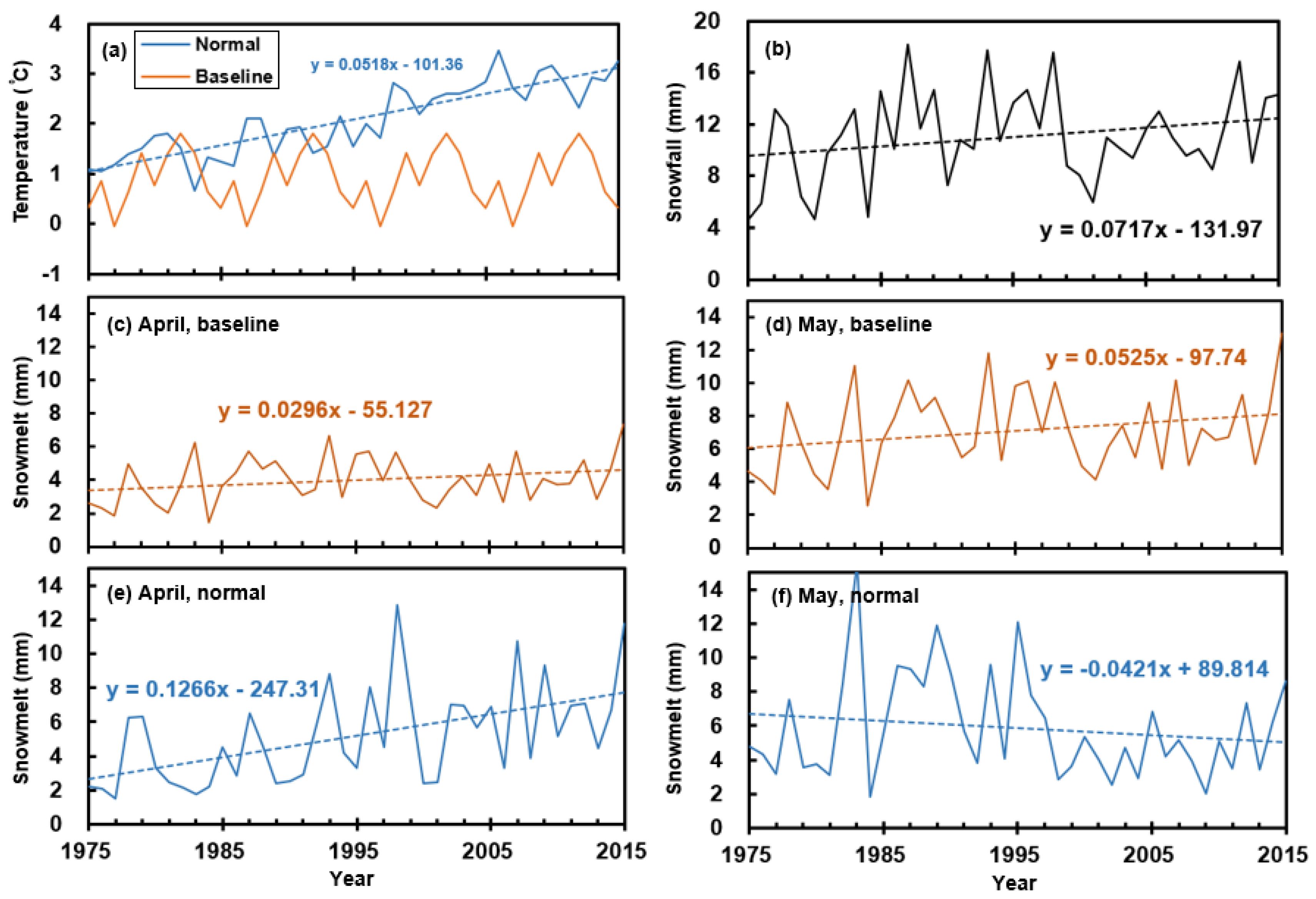
With increasing in the air temperature during 1975–2015, the annual snowmelt runoff in the study catchment showed an increasing trend and a change in seasonal distribution. The concentrated release period of the snowmelt runoff gradually shifted from May to April. The spring flood in the Golmud River will shorten the time while raise the peak.

(3)

The ABCD-CR model can capture the increasing effect of the hydraulic conductivity of soils with the frozen soil degradation caused by the global warming. As revealed, the frozen soil degradation led to an increase in the cold season runoff whereas did not affect the warm season runoff.

(4)

The annual runoff in the headwater catchment of the Golmud River was positively correlated with the groundwater level in the area of the Golmud city. The increasing streamflow in the Golmud River was the major cause for the rising groundwater level in the Golmud city over the past 20 years.

The model developed in this study may provide a useful tool for analyzing the changes in the catchment scale runoff in cold regions triggered by the climate change.

References

1. Viviroli, D.; Dürr, H.H.; Messerli, B.; Meybeck, M.; Weingartner, R. Mountains of the world, water towers for humanity: Typology, mapping, and global significance. Water Resour. Res. 2007, 43. [Google Scholar] [CrossRef] [Green Version]
2. Apel, H.; Thieken, A.H.; Merz, B.; Blöschl, G. A Probabilistic Modelling System for Assessing Flood Risks. Nat. Hazards 2006, 38, 79–100. [Google Scholar] [CrossRef]
3. Ignacio, J.A.F.; Cruz, G.T.; Nardi, F.; Henry, S. Assessing the effectiveness of a social vulnerability index in predicting heterogeneity in the impacts of natural hazards: Case study of the Tropical Storm Washi flood in the Philippines. Vienna Yearb. Popul. Res. 2016, 13, 91–129. [Google Scholar] [CrossRef] [Green Version]
4. Nardi, F.; Morrison, R.R.; Annis, A.; Grantham, T.E. Hydrologic scaling for hydrogeomorphic floodplain mapping: Insights into human-induced floodplain disconnectivity. River Res. Appl. 2018, 34, 675–685. [Google Scholar] [CrossRef]
5. Immerzeel, W.W.; van Beek, L.P.H.; Bierkens, M.F.P. Climate change will affect the Asian water towers. Science 2010, 328, 1382–1385. [Google Scholar] [CrossRef]
6. Liu, X.; Chen, B. Climatic warming in the Tibetan Plateau during recent decades. Int. J. Climatol. 2000, 20, 1729–1742. [Google Scholar] [CrossRef]
7. Guo, D.; Wang, H. The significant climate warming in the northern Tibetan Plateau and its possible causes. Int. J. Climatol. 2012, 32, 1775–1781. [Google Scholar] [CrossRef]
8. Zhu, X.; Wang, W.; Fraedrich, K. Future Climate in the Tibetan Plateau from a Statistical Regional Climate Model. J. Clim. 2013, 26, 10125–10138. [Google Scholar] [CrossRef] [Green Version]
9. Song, C.; Pei, T.; Zhou, C. The role of changing multiscale temperature variability in extreme temperature events on the eastern and central Tibetan Plateau during 1960–2008. Int. J. Climatol. 2014, 34, 3683–3701. [Google Scholar] [CrossRef]
10. Cai, D.; You, Q.; Fraedrich, K.; Guan, Y. Spatiotemporal Temperature Variability over the Tibetan Plateau: Altitudinal Dependence Associated with the Global Warming Hiatus. J. Clim. 2017, 30, 969–984. [Google Scholar] [CrossRef]
11. Wan, G.; Yang, M.; Liu, Z.; Wang, X.; Liang, X. The Precipitation Variations in the Qinghai-Xizang (Tibetan) Plateau during 1961–2015. Atmosphere 2017, 8, 80. [Google Scholar] [CrossRef] [Green Version]
12. Immerzeel, W.W.; van Beek, L.P.; Konz, M.; Shrestha, A.B.; Bierkens, M.F. Hydrological response to climate change in a glacierized catchment in the Himalayas. Clim. Chang. 2012, 110, 721–736. [Google Scholar] [CrossRef] [PubMed] [Green Version]
13. Guo, D.; Wang, H. Simulation of permafrost and seasonally frozen ground conditions on the Tibetan Plateau, 1981–2010. J. Geophys. Res. Atmos. 2013, 118, 5216–5230. [Google Scholar] [CrossRef]
14. Shen, M.; Zhang, G.; Cong, N.; Wang, S.; Kong, W.; Piao, S. Increasing altitudinal gradient of spring vegetation phenology during the last decade on the Qinghai–Tibetan Plateau. Agric. For. Meteorol. 2014, 189–190, 71–80. [Google Scholar] [CrossRef]
15. Qin, Y.; Lei, H.; Yang, D.; Gao, B.; Wang, Y.; Cong, Z.; Fan, W. Long-term change in the depth of seasonally frozen ground and its ecohydrological impacts in the Qilian Mountains, northeastern Tibetan Plateau. J. Hydrol. 2016, 542, 204–221. [Google Scholar] [CrossRef]
16. Qin, Y.; Yang, D.; Gao, B.; Wang, T.; Chen, J.; Chen, Y.; Wang, Y.; Zheng, G. Impacts of climate warming on the frozen ground and eco-hydrology in the Yellow River source region, China. Sci. Total Environ. 2017, 605–606, 830–841. [Google Scholar] [CrossRef] [Green Version]
17. Zhang, W.; Yi, Y.; Song, K.; Kimball, J.S.; Lu, Q. Hydrological Response of Alpine Wetlands to Climate Warming in the Eastern Tibetan Plateau. Remote. Sens. 2016, 8, 336. [Google Scholar] [CrossRef] [Green Version]
18. Kang, S.; Xu, Y.; You, Q.; Flügel, W.-A.; Pepin, N.; Yao, T. Review of climate and cryospheric change in the Tibetan Plateau. Environ. Res. Lett. 2010, 5, 15101. [Google Scholar] [CrossRef]
19. Walvoord, M.A.; Kurylyk, B.L. Hydrologic Impacts of Thawing Permafrost—A Review. Vadose Zone J. 2016, 15. [Google Scholar] [CrossRef]
20. Cuo, L.; Zhang, Y.; Bohn, T.J.; Zhao, L.; Li, J.; Liu, Q.; Zhou, B. Frozen soil degradation and its effects on surface hydrology in the northern Tibetan Plateau. J. Geophys. Res. Atmos. 2015, 120, 8276–8298. [Google Scholar] [CrossRef] [Green Version]
21. Yang, H.; Yang, D. Derivation of climate elasticity of runoff to assess the effects of climate change on annual runoff. Water Resour. Res. 2011, 47. [Google Scholar] [CrossRef]
22. Yang, H.; Qi, J.; Xu, X.; Yang, D.; Lv, H. The regional variation in climate elasticity and climate contribution to runoff across China. J. Hydrol. 2014, 517, 607–616. [Google Scholar] [CrossRef]
23. Yao, T.; Xue, Y.; Chen, D.; Chen, F.; Thompson, L.; Cui, P.; Koike, T.; Lau, W.K.-M.; Lettenmaier, D.; Mosbrugger, V.; et al. Recent Third Pole’s Rapid Warming Accompanies Cryospheric Melt and Water Cycle Intensification and Interactions between Monsoon and Environment: Multidisciplinary Approach with Observations, Modeling, and Analysis. Bull. Am. Meteorol. Soc. 2019, 100, 423–444. [Google Scholar] [CrossRef]
24. Cuo, L.; Zhang, Y.; Zhu, F.; Liang, L. Characteristics and changes of streamflow on the Tibetan Plateau: A review. J. Hydrol. 2014, 2, 49–68. [Google Scholar] [CrossRef] [Green Version]
25. Sichangi, A.W.; Wang, L.; Yang, K.; Chen, D.; Wang, Z.; Li, X.; Zhou, J.; Liu, W.; Kuria, D. Estimating continental river basin discharges using multiple remote sensing data sets. Remote Sens. Environ. 2016, 179, 36–53. [Google Scholar] [CrossRef] [Green Version]
26. Gleason, C.; Smith, L. Toward Global Mapping of River Discharge Using Satellite Images and At-Many-Stations Hydraulic Geometry. Proc. Natl. Acad. Sci. USA 2014, 111, 4788–4791. [Google Scholar] [CrossRef] [Green Version]
27. Bomers, A.; van der Meulen, B.; Schielen, R.M.J.; Hulscher, S.J.M.H. Historic Flood Reconstruction with the Use of an Artificial Neural Network. Water Resour. Res. 2019, 55, 9673–9688. [Google Scholar] [CrossRef] [Green Version]
28. Kratzert, F.; Klotz, D.; Brenner, C.; Schulz, K.; Herrnegger, M. Rainfall—Runoff modelling using Long Short-Term Memory (LSTM) networks. Hydrol. Earth Syst. Sci. 2018, 22, 6005–6022. [Google Scholar] [CrossRef] [Green Version]
29. Wang, L.; Koike, T.; Yang, K.; Jin, R.; Li, H. Frozen soil parameterization in a distributed biosphere hydrological model. Hydrol. Earth Syst. Sci. 2009, 14, 557–571. [Google Scholar] [CrossRef] [Green Version]
30. Qi, J.; Wang, L.; Zhou, J.; Song, L.; Li, X.; Zeng, T. Coupled Snow and Frozen Ground Physics Improves Cold Region Hydrological Simulations: An Evaluation at the upper Yangtze River Basin (Tibetan Plateau). J. Geophys. Res. Atmos. 2019, 124, 12985–13004. [Google Scholar] [CrossRef]
31. Gao, B.; Yang, D.; Qin, Y.; Wang, Y.; Li, H.; Zhang, Y.; Zhang, T. Change in frozen soils and its effect on regional hydrology, upper Heihe basin, nor theastern Qinghai—Tibetan Plateau. Cryosphere 2018, 12, 657–673. [Google Scholar] [CrossRef] [Green Version]
32. Liu, B.; Quan, J.; Yang, C.; Lei, X.; Wang, H. Simulation of runoff of major basins in Qinghai Province based on SWAT model. Water Resour. Prot. 2016, 32, 39–44. (In Chinese) [Google Scholar] [CrossRef]
33. De Paola, F.; Giugni, M.; Pugliese, F.; Annis, A.; Nardi, F. GEV Parameter Estimation and Stationary vs. Non-Stationary Analysis of Extreme Rainfall in African Test Cities. Hydrology 2018, 5, 28. [Google Scholar] [CrossRef] [Green Version]
34. Guo, D.; Westra, S.; Maier, H.R. An inverse approach to perturb historical rainfall data for scenario-neutral climate impact studies. J. Hydrol. 2018, 556, 877–890. [Google Scholar] [CrossRef]
35. Budyko, M.I. (Ed.) Climate and Life; Elsevier: New York, NY, USA, 1974. [Google Scholar]
36. Wu, P.; Liang, S.; Wang, X.-S.; Feng, Y.; McKenzie, J.M. Climate-induced hydrologic change in the source region of the Yellow River: A new assessment including varying permafrost. Water 2018, 10, 877. [Google Scholar] [CrossRef] [Green Version]
37. Wang, T.; Yang, H.; Yang, D.; Qin, Y.; Wang, Y. Quantifying the streamflow response to frozen ground degradation in the source region of the Yellow River within the Budyko framework. J. Hydrol. 2018, 558, 301–313. [Google Scholar] [CrossRef]
38. Gao, B.; Qin, Y.; Wang, Y.; Yang, D.; Zheng, Y. Modeling Ecohydrological Processes and Spatial Patterns in the Upper Heihe Basin in China. Forests 2016, 7, 10. [Google Scholar] [CrossRef] [Green Version]
39. Zheng, D.; van der Velde, R.; Su, Z.; Wen, J.; Wang, X.; Yang, K. Impact of soil freeze-thaw mechanism on the runoff dynamics of two Tibetan rivers. J. Hydrol. 2018, 563, 382–394. [Google Scholar] [CrossRef]
40. Kirchner, J.W. Getting the right answers for the right reasons: Linking measurements, analyses, and models to advance the science of hydrology. Water Resour. Res. 2006, 42. [Google Scholar] [CrossRef]
41. Thomas, H.A. Improved Methods for National Water Assessment; US Water Resources Council: Washington, DC, USA, 1981.
42. Alley, W.M. Treatment of evapotranspiration, soil moisture accounting and aquifer recharge in monthly water balance models. Water Resour. Res. 1984, 1137–1149. [Google Scholar] [CrossRef]
43. Zhao, J.; Wang, D.; Yang, H.; Sivapalan, M. Unifying catchment water balance models for different time scales through the maximum entropy production principle. Water Resour. Res. 2016, 52, 7503–7512. [Google Scholar] [CrossRef]
44. Sankarasubramanian, A.; Vogel, R.M. Annual hydroclimatology of the United States. Water Resour. Res. 2002, 38, 19-11–19-12. [Google Scholar] [CrossRef]
45. Wang, X.-S.; Zhou, Y. Shift of annual water balance in the Budyko space for catchments with groundwater-dependent evapotranspiration. Hydrol. Earth Syst. Sci. 2016, 20, 3673–3690. [Google Scholar] [CrossRef] [Green Version]
46. Han, P.; Wang, X. Forecasting the response of a catchment on extreme climate change with ABCD model. Yellow River 2016, 38, 16–21. (In Chinese) [Google Scholar]
47. Martinez, G.F.; Gupta, H.V. Toward improved identification of hydrological models: A diagnostic evaluation of the “abcd” monthly water balance model for the conterminous United States. Water Resour. Res. 2010, 46, W08507. [Google Scholar] [CrossRef]
48. Yuan, X.; Liu, S.; Tian, G.; Chen, L.; Yu, J. Analysis of the fractal dimension in the Golmud River basin based on DEM. Remote. Sens. Land Resour. 2013, 25, 111–116. (In Chinese) [Google Scholar]
49. Li, L.; Ni, W.; Li, T.; Zhou, B.; Qu, Y.; Yuan, K. Influences of anthropogenic factors on lakes area in the Golmud Basin, China, from 1980 to 2015. Environ. Earth Sci. 2019, 79. [Google Scholar] [CrossRef]
50. Ma, S.; Xu, L. Analysis on the causes and climate of the Golmud River Basin in summer of 2010. Qinghai Sci. Technol. 2011, 18, 38–41. (In Chinese) [Google Scholar]
51. Xu, A.; Zhang, H. Construction technique for emergency risk-elimination of Wenquan Reservoir on Golmud River. Water Resour. Hydropower Eng. 2011, 42, 44–45. (In Chinese) [Google Scholar]
52. Wang, S.; Wang, W.; He, H.; Shen, C. Analysis of riverbed infiltration capacity of Golmud River. Shanxi Archit. 2016, 42, 99–100. (In Chinese) [Google Scholar]
53. Tan, H.; Liu, X.; Yu, S.; Lu, Y. Character of Hydrochemistry in Golmud River-Dabsan Lake Water. J. Lake Sci. 2001, 13, 43–50. (In Chinese) [Google Scholar]
54. Wang, S.; Wang, X. Causes and environmental geology effects of inter-annual groundwater level variations in the Golmud city, China. Geotech. Investig. Surv. 2019, 6, 36–42. (In Chinese) [Google Scholar]
55. Abatzoglou, J.T.; Dobrowski, S.Z.; Parks, S.A.; Hegewisch, K.C. TerraClimate, a high-resolution global dataset of monthly climate and climatic water balance from 1958–2015. Sci. Data. 2018, 5, 170191. [Google Scholar] [CrossRef] [Green Version]
56. Li, J.; Shao, Y.; Wang, Q.; Zhang, H. Comparative analysis of E601B evaporation and small evaporatopm observation data in Qinghai Province. Qinghai Sci. Technol. 2006, 13, 52–55. (In Chinese) [Google Scholar] [CrossRef]
57. Liu, M.; Shen, Y.; Zeng, Y.; Liu, C. Changing trend of pan evaporation and its cause over the past 50 years in China. Acta Geogr. Sin. 2009, 64, 259–269. (In Chinese) [Google Scholar] [CrossRef]
58. Zhang, Q.; Qi, T.; Li, J.; Singh, V.P.; Wang, Z. Spatiotemporal variations of pan evaporation in China during 1960-2005: Changing patterns and causes. Int. J. Climatol. 2015, 35, 903–912. [Google Scholar] [CrossRef]
59. Roderick, M.L.; Farquhar, G.D. The cause of decreased pan evaporation over the past 50 years. Science 2002, 298, 1410–1411. [Google Scholar] [CrossRef]
60. Woo, M.-K. Permafrost Hydrology; Springer: New York, NY, USA, 2012. [Google Scholar] [CrossRef]
61. Refshaard, J.C.; Storm, B. (Eds.) MIKE SHE, in Computer Models of Watershed Hydrology; Water Resources Publications: Highlands Ranch, CO, USA, 1995; pp. 809–846. [Google Scholar]
62. Nash, J.E.; Sutcliffe, J.V. River flow forecasting through conceptual models part I—A discussion of principles. J. Hydrol. 1970, 10, 282–290. [Google Scholar] [CrossRef]
63. Wang, L.; Sichangi, A.W.; Zeng, T.; Li, X.; Hu, Z.; Genanu, M. New methods designed to estimate the daily discharges of rivers in the Tibetan Plateau. Sci. Bull. 2019, 64, 418–421. [Google Scholar] [CrossRef] [Green Version]
64. Kou, W. The Conversion between Surface Water and Groundwater and the Retional Exploitation in Golmud Basin. Master’s Dissertation, China University of Geosciences, Beijing, China, 2006. [Google Scholar]
65. Kong, N.; Qu, T.; Tan, H.; Zhang, W.; Zhang, Y. Distribution of Isotopes and Runoff Variation of the Rivers in the Qaidam Basin. Arid Zone Res. 2014, 5, 948–954. (In Chinese) [Google Scholar] [CrossRef]
66. Wen, G.; Wang, W.; Duan, L.; Li, Y.; Zhao, J. Response of runoff to climate change and human activity in the upper reaches of the Bayin River, Qaidam Basin, Qinghai Province. J. Glaciol. Geocryol. 2018, 40, 136–144. (In Chinese) [Google Scholar] [CrossRef]
Figure 1. Study area and locations of the meteorological and hydrological stations.
Water 12 01812 g001
Figure 2. Mean monthly precipitation observed at typical meteorological stations and extracted from TERRACLIMATE data: (a) the Qumarleb meteorological station; (b) the Golmud meteorological station.
Water 12 01812 g002
Figure 3. Variations of the annual precipitation, annual potential evaporation and annual mean air temperature in the study catchment, at the basin-scale in average.
Water 12 01812 g003
Figure 4. Locations of hydrological stations and observation wells (a) with available groundwater level data (b). Streamflow observed at W-IV (c) and W-III (d) in different periods. Dashed line in (c) denotes the restored streamflow at W-III obtained by considering the leakage of river water between W-III and W-IV [54]. The annual precipitation at the Golmud city is also shown as histograms in (c) and (d).
Water 12 01812 g004
Figure 5. Outlines of models: (a) the ABCD model; (b) the Modified ABCD Model for Cold Regions (ABCD-CR) model.
Water 12 01812 g005
Figure 6. Monthly runoff results of the study catchment in the calibration and validation period obtained from the ABCD-CR model.
Water 12 01812 g006
Figure 7. Monthly runoff results of the study catchment in the calibration and validation period obtained from (a) the ABCD model, (b) the ABCD-I model, and (c) the ABCD-II model.
Water 12 01812 g007
Figure 8. Annual precipitation and potential evaporation (a) and the restored annual runoff from different models (b).
Water 12 01812 g008
Figure 9. Restoring results of the monthly runoff in the study catchment (b) with meteorological data in the period 1990–2015 (a).
Water 12 01812 g009
Figure 10. Comparable data and results for the normal and baseline simulations: (a) The annual mean air temperature; (b) the annual snowfall; (c,e) are the snowmelt runoff in April from the normal simulation and baseline simulation, respectively; (d,f) are the snowmelt runoff in May from the normal simulation and baseline simulation, respectively.
Water 12 01812 g010
Figure 11. The trend of air temperature’s change in warm season (a) and cold season (b); The comparison of runoff with normal simulation and baseline simulation in warm season (c) and cold season (d).
Water 12 01812 g011
Figure 12. Correlation between the simulated annual runoff in the study catchment and observed groundwater level in G1 (a), G2 (b), G3 (c)and G4 (d) (Figure 4b).
Water 12 01812 g012