Experimental and Numerical Investigations of Hydraulics in Water Intake with Stop-Log Gate

Abstract

A stop-log gate, installed in water intake of hydropower project, has become an effective facility in achieving selective withdrawal and temperature control for the sake of benefiting downstream ecosystems. Hence, it is of great importance to comprehensively explore the water intake hydraulics with the gate, not limited to some specific case studies. This study deals, through laboratory experiments and numerical simulations, with flow features of such a gate-functioned intake. The physical model test is used to validate the numerical simulation. Subsequently, a series of numerical cases considering different hydraulic and geometric conditions are performed to help look into the behaviors. Particular attention is paid to the flow regimes, head loss and flow velocity distributions. The results showcase the effect of the gate on the intake flow regime, and in terms of head loss and flow velocity distribution, the influences of the upstream water head, intake chamber width and withdrawal depth are revealed in detail. An empirical expression, with regard to the coefficient of head loss, is derived and validated by data from the available literature. Moreover, it is found that the maximum velocity at trash rack section is dependent exclusively on the relative withdrawal depth and always occurs at a certain height range above the gate. These results may provide a meaningful reference for the research of water intake with similar situations.

1. Introduction

In the past decades, large quantities of hydropower stations and man-made reservoirs have been constructed to achieve efficient utilization of water resources. However, these infrastructures are inevitably destroying the balance of reservoir ecology and surface runoff [1]. Most reservoirs with a large depth are typically temperature stratified. As a result, temperature variance of reservoirs significantly affects the downstream ecosystem, ecological diversity and agricultural irrigation [2,3,4,5]. Therefore, the temperature management has been a great concern for designers and operators [6,7]. To this end, selective water withdrawal from different depths of a reservoir is widely adopted, and different facilities are developed to achieve the selective withdrawal, e.g., the stop-log gate and the temperature-control curtain [8,9].

Stop-log gates are originally designed as typical closure systems for dewater spillway gates in many dams [10]. At present, they are employed for water intake to achieve selective withdrawal and mitigate the outflow temperature problem in many hydropower projects, e.g., Jingping-I, Guangzhao, Baihetan, Nuozhadu, etc. [11]. In the vicinity of the water intake, a stop-log gate forces all released water to originate from layers above the gate. According to previous studies, the gate is manifested as an effective facility to regulate the outflow temperatures. Meanwhile, flow patterns at the intake are also affected significantly by the gate, sometimes leading to undesirable flow performance. For example, it is reported that stop-log gates cause a 1–2 m head loss, resulting in an annual power loss of 26 million kW·h in Guangzhao Hydropower Station [12].

Previous studies on the selective withdrawal intake primarily concentrate on the thermal dynamic characteristics. On the basis of water temperature and quality model, much attention has been paid to the change of outflow temperature and related water quality when selective withdrawal facilities are applied [13,14,15,16]. Researchers have carried out extensive work on the hydraulics of stop-log gate. In the experimental field, Vermeyen [17,18] reports a case study on the head loss, vortices formation, velocity distribution, critical submergence depth, forand Clen Canyon Dam. Zhang et al. [19] investigate the effect of stop-log gate height on flow behaviors, water temperature and oxygen content in Bakun Hydropower Station in Malaysia. Similar model tests are also performed for projects such as Guangzhao, Nuozhadu and Jinping-I. Some qualitative findings, in terms of flow regime, head loss, velocity distribution and surface vortices are obtained [20,21,22]. In the numerical field, different turbulence models are applied to simulate the flow at water intake with CFD software, e.g., Fluent [16,23]. Li adopts a 3D model to simulate and summarize the head loss, velocity distribution, flow pattern at selective withdrawal intake in Nuozhadu project. The results demonstrate a fairly good agreement with experimental results and consequently the effectiveness of such method [24].

Regarding the hydraulic characteristics of water intake with a stop-log gate, limitations do exist, in spite of some available explorations. Most of the existing studies are based on specific project cases, in which certain design parameters are investigated rather than a systematic study when the gate is in operation. Imposed by practical constraints, prototype observations and measurements are challengeable to make; physical model test and numerical simulation, as favorable alternatives, complement each other and are capable of exploring the behaviors comprehensively.

This study is motivated by the need to understand the effect of stop-log gate on the hydraulic characteristics of a water intake. Both physical experiments and numerical models are performed to investigate the flow features, especially for the flow regime, head loss and velocity distribution. In addition to comparing the numerical results with experimental measurements, a number of cases with different hydraulic and geometric parameters are also examined. The study addresses the stop-log gate hydraulics and the results are reported in the form of non-dimensional parameters, thereby providing guidance for engineering applications.

2. Methodology

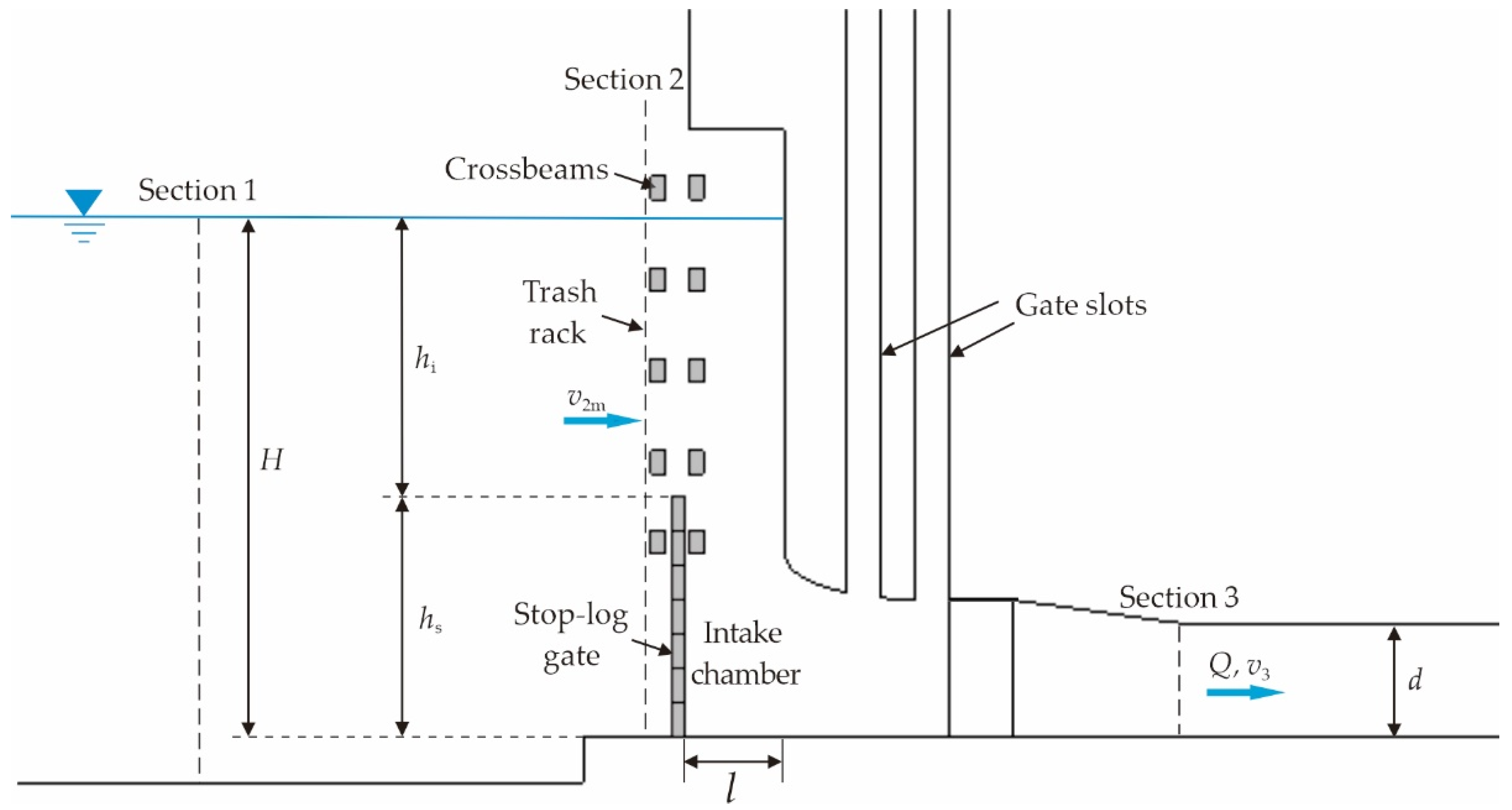
2.1. Theoretical Considerations

To achieve the water withdrawal from different layers, a stop-log gate with adjustable height is designed. Figure 1 shows the sketch of the intake geometry. Three sections are selected to help illustrate the flow features: Section 1 is placed upstream of the water intake in the reservoir, where the water level is not disturbed; Section 2 is in the place of trash rack, 2 m upstream of the stop-log gate, and Section 3 is downstream of tunnel transaction, where the flow reaches a stable state. The geometric parameters contain h_s (m) as the height of the stop-log gate, l (m) as the width of intake chamber and d (m) as the diameter of the withdrawal tunnel. The hydraulic parameters are total water head H (m) in reservoir, withdrawal depth above the stop-log gate h_i = H − h_s (m), withdrawal discharge Q (m³/s) and averaged flow velocity v₃ (m/s) in Section 3.

The water head loss ΔH (m), between Section 1 and Section 3, is an essential parameter for evaluation of the water intake. The main factors that affect the ΔH include:

$$\Delta H=f\left(H,h_i,l,Q,d,g\right)$$

(1)

where g (m/s²) is the gravitational acceleration. Selecting Q, g and d as the independent basic quantities and using Buckingham Π theorem, Equation (1) is simplified into:

$$\xi =f\left[\frac{H}{d},\frac{h_i}{d},\frac{l}{d}\right]$$

(2)

where ξ is defined as the dimensionless coefficient of head loss. It indicates that the ξ is a function of H/d, h_i/d and l/d and reads as

$$\xi =\frac{\Delta H}{v^2/2g}=\frac{\Delta H}{8Q^2/g{\left(\pi d^2\right)}^2}$$

(3)

The Equation (3) is consistent with the earlier work [20,24,25,26], and it is widely acknowledged, thus a reasonable comparison can be made in the present work.

2.2. Numerical Simulation

Based on the Fluent package in ANSYS (ANSYS Inc., Canonsburg, PA, USA) [27], a numerical model is set up to help understand the complex flow features of the water intake.

2.2.1. Governing Equations

The flow field is governed by the incompressible viscous Navier–Stokes equations [27]. The turbulence effectsre modelled by a URANS method, which is based on the Boussinesq’s assumption. The finite-volume method is used to discrete the flow domain and governing equations with second-order accuracy [27]. The governing equations are given as:

Continuity equation:

$$\frac{\partial U_i}{\partial X_i}=0$$

(4)

Momentum equation:

$$\frac{\partial U_i}{\partial t}+\frac{\partial (U_i{U}_j)}{\partial X_j}=-\frac{1}{\rho }\frac{\partial P}{\partial X_i}+\frac{\partial }{\partial X_j}\left(\nu \frac{\partial U_i}{\partial X_j}+{\tau }_{ij}\right)+\frac{1}{\rho }{F}_i$$

(5)

where t is time; U_i and U_j are velocity components in the X_i and X_j directions; P is pressure; ρ is water density; v is kinematic viscosity coefficient; ${\tau }_{ij}$ is the specific Reynolds stress tensor; F_i is the body force in the X_i direction. X_i, X_j and X_k stand for the X, Y and Z directions, respectively.

The Volume of Fluid method (VOF) is used to simulate the free surface. The method is proposed by Hirt and Nichols [28], which is a free-surface technique. Based on the Eulerian method, a fixed mesh is applied to track the shape and position of the interface between air and water. The VOF for each fluid is calculated throughout the domain. The water is usually defined as a primary phase, and the air is a secondary phase.

According to previous studies (e.g., Jothiprakash et al. [29], Teng et al. [30], Zhang et al. [31]), the RNG κ-ε turbulence model is capable of achieving a good balance between prediction accuracy and computational cost, compared to those computationally expensive Large Eddy Simulations (LES). This model is more suitable for representing free-surface flows. The standard wall functions are used to avoid resolving the turbulent boundary layers, which do not play an important role in this hydraulic simulation. Kinetic energy κ and turbulent dissipation rate ε are obtained by:

$$\frac{\partial \kappa }{\partial t}+U_j\frac{\partial \kappa }{\partial X_j}=\frac{\partial }{\partial X_j}\left[(\nu +\frac{{\nu }_t}{{\sigma }_{\kappa }})\frac{\partial \kappa }{\partial X_j}\right]+{\tau }_{ij}\frac{\partial U_i}{\partial X_j}-\epsilon$$

(6)

$$\frac{\partial \epsilon }{\partial t}+U_j\frac{\partial \epsilon }{\partial X_j}=\frac{\partial }{\partial X_j}\left[(\nu +\frac{{\nu }_t}{{\sigma }_{\epsilon }})\frac{\partial \epsilon }{\partial X_j}\right]+C_{\epsilon 1}{\tau }_{ij}\frac{\epsilon }{\kappa }\frac{\partial U_i}{\partial X_j}-C_{\epsilon 2}\frac{{\epsilon }^2}{\kappa }$$

(7)

where ${\nu }_t$ is kinematic eddy viscosity ${\nu }_t=\frac{C_{\mu }{\kappa }^2}{\epsilon },C_{\mu }=0.09,{\sigma }_k=1.0,{\sigma }_{\epsilon }=1.3,C_{\epsilon 1}=1.44$ and $C_{\epsilon 2}=1.92$.

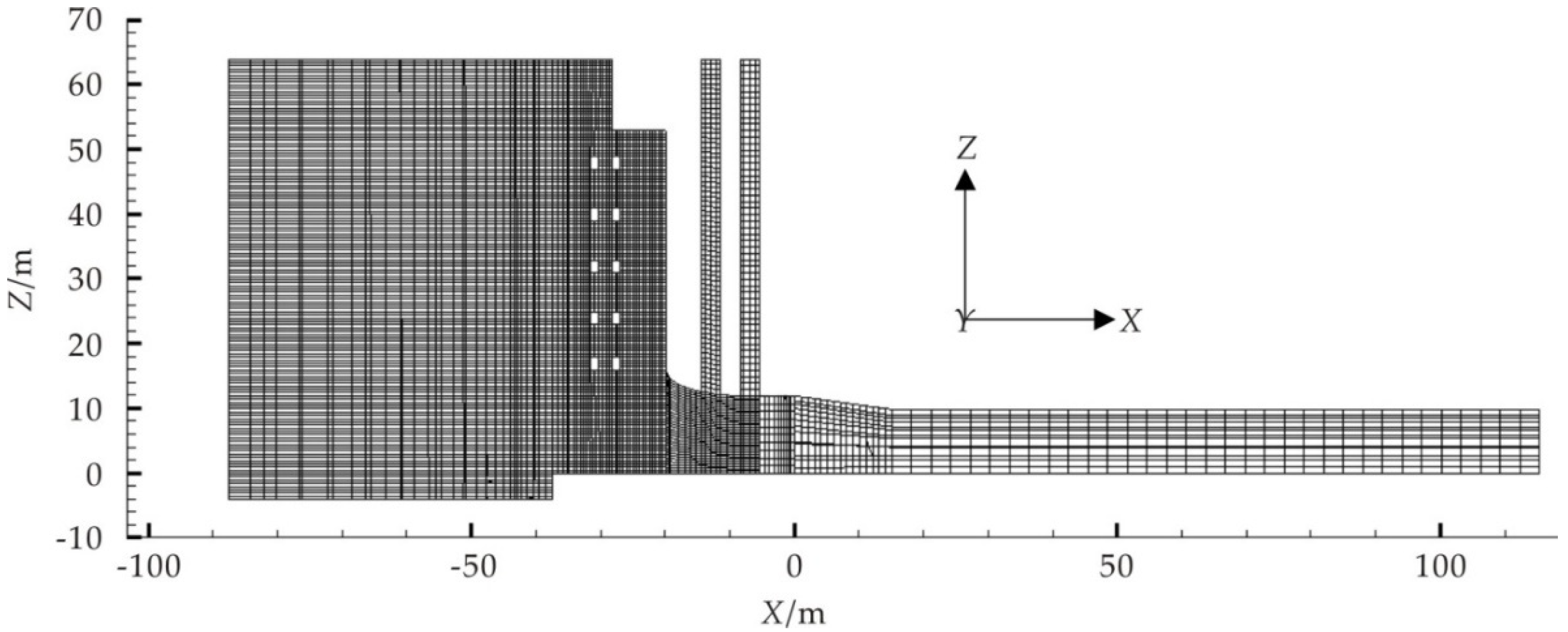
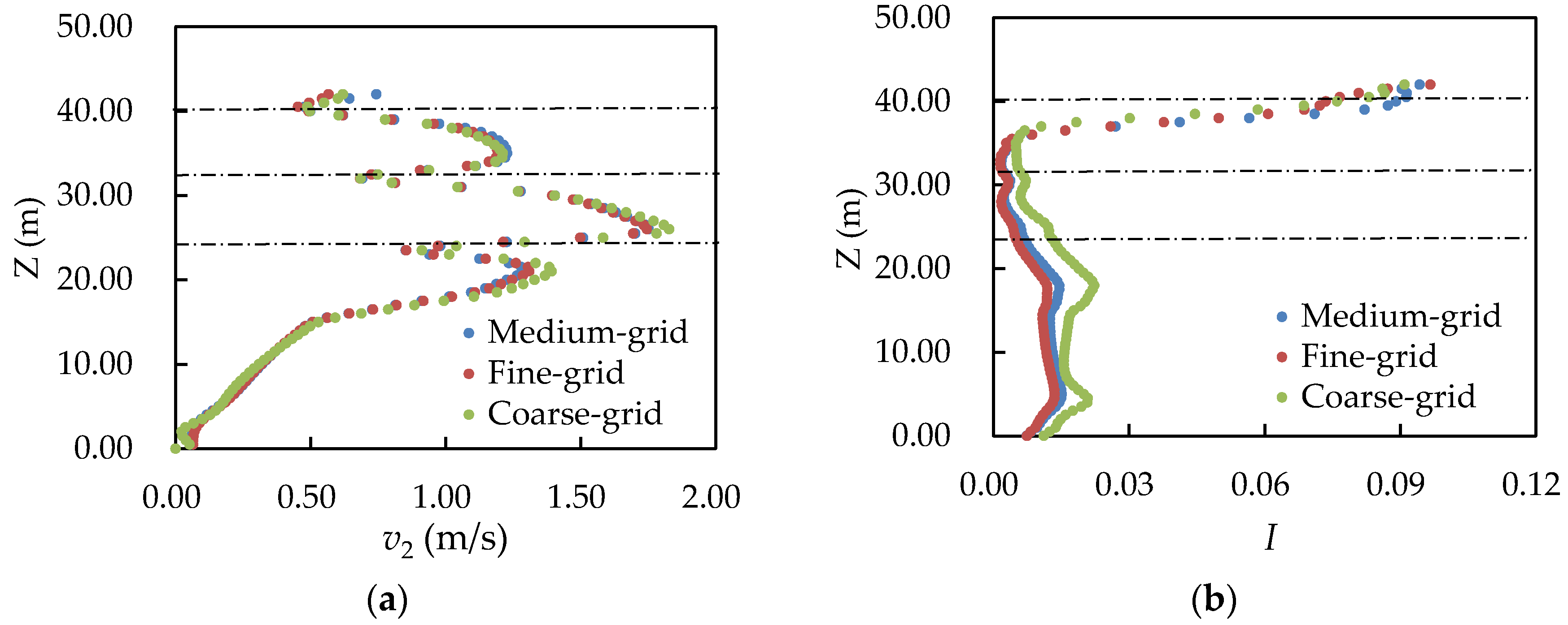
2.2.2. Model Setup

The computational domain and numerical grid are illustrated in Figure 2, in which a 3D coordinate system (X, Y, Z) is defined. The X-coordinate is along the water intake bottom (positive downwards); the Y-coordinate is placed perpendicular to the X (positive leftside), and the Z-coordinate is positioned perpendicular to the X and Y plane (positive upwards). The grid is generated using the ICEM. The domain length is 200 m. In the vicinity of the gate and close to the water intake, the grid density level is higher. A quality grid is the prerequisite for reliable simulations. To guarantee the numerical quality, a check of grid independence is necessary. Grid independence is checked through steady-state flow calculations. Three quadrilateral grids are examined, with the number of cells being about 150,000 (coarse), 260,000 (medium), and 400,000 (fine), respectively, and corresponding to the average cell size of approximately 0.70, 0.40 and 0.25 m. For the grid independence check, the velocity v₂ and turbulent intensity I are compared. I = U′/U_mean, where U′ and U_mean denote the root-mean-square of the velocity fluctuations and mean flow velocity, respectively. The comparison is shown in Figure 3. The dotted lines represent the position of cross-beams. The results indicate that the medium size grid is sufficient to model the water intake flow. For the whole domain, it is finally divided into 260,000 hexahedral cells.

Regarding the definition of boundary conditions, the upstream boundary is specified with a pressure inlet corresponding to the water depth and air pressure with the atmospheric pressure. The downstream boundary is defined as a velocity inlet, corresponding to the average outflow at the Section 3. Negative value denotes that the flow runs out of the domain. The upper boundary is set as pressure inlets. The turbulence conditions at the inlets are expressed in terms of turbulence intensity level and turbulence viscosity ratio; their embedded values in the program are 3% and 5, respectively, which are typical for inlet conditions [32,33]. The solid (concrete) boundaries, including the reservoir bottom and all the surrounded walls are treated as walls, with no-slip condition irrespective of phase. The free surface is assumed to be a smooth surface without any water level fluctuations. There is intermittent air engulfment observed at the free surface when the water withdrawal depth is small, i.e., ≤15 m. To eliminate the effect of air engulfment, the study is performed with the withdrawal depth in the range of 18–30 m. The values of some parameters adopted in the model are listed in

Table 1. Parameter values adopted in the model.

Parameter	Cμ	C1ε	C2ε	σk	σε
Value	0.09	1.44	1.92	1.00	1.30

.

In the simulations, 18 cases are taken into account with respect to the H, l and h_i, as listed in

Table 2. Simulated cases with different H, l and h_i.

Cases	1	2	3	4	5	6	7	8	9	10	11	12	13	14	15	16	17	18
H (m)	36	39	42	45	48	51	54	57	42	42	42	42	42	42	42	42	42	42
l (m)	7	7	7	7	7	7	7	7	8	9	10	11	13	15	7	7	7	7
hi (m)	21	21	21	21	21	21	21	21	21	21	21	21	21	21	18	24	27	30

. All the cases are subjected to the same inlet flow Q = 372.48 m³/s and d = 10 m. To look into the effect of H, cases 1–8 are designed with varied H = 36–57 m; at the given H = 42 m, h_i = 21 m, the cases 3, 9–14 are performed with varied l = 8–15 m; for cases 3, 15–18, the effect of h_i is examined.

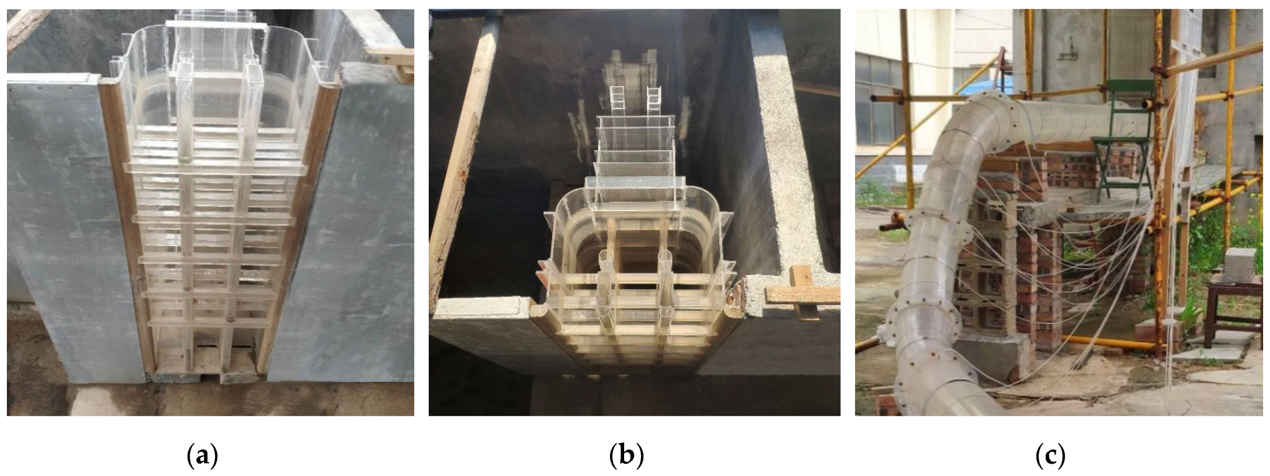
2.3. Experimental Tests

The experiments are performed in the Hydraulic Laboratory of Zhongnan Engineering Corporation Limited in Changsha, China. The experimental layout is shown in Figure 4. It consists of a pump, an approach conduit, a large feeding basin, a physical model and a flow return system. Based on the Froude similarity criterion, the physical model is designed at a scale of 1/40, which is also in consideration of previous research and the laboratory site conditions [34]. In terms of the intake hydraulic model, the scale ratio of 1:50 to 1:100 is acceptable. Therefore, the induced scale effects in our study subjected to 1:40, are negligibly small. The model consists of a model reservoir, a selective withdrawal intake with a stop-log gate and a connecting tunnel. The crossbeams in two layers are placed in the water intake, with the stop-log gate in between, also marked in Figure 1. There are 10 crossbeams in total, and the centerline distance two beams in vertical direction is 8 m. Water is supplied by pumping it from an underground reservoir. A discharge measured weir is equipped at the end of the flow return system.

The water level in the reservoir (Section 1) is measured by stylus, with an error of ±0.1 cm. The velocity v₂ (m/s) at Section 2 is measured through LGY-Ⅱ flowmeter, with an error of ≤1.5%. At the connecting tunnel (Section 3), four points in a circumference are arranged with manometers to measure the pressure head p (m) and velocity head p_v (m). Preliminary trials prove that the physical model shows acceptable reproducibility. To minimize the error, for each case investigated, five parallel measurements are carried out to eliminate the measurement uncertainty.

3. Results and Discussions

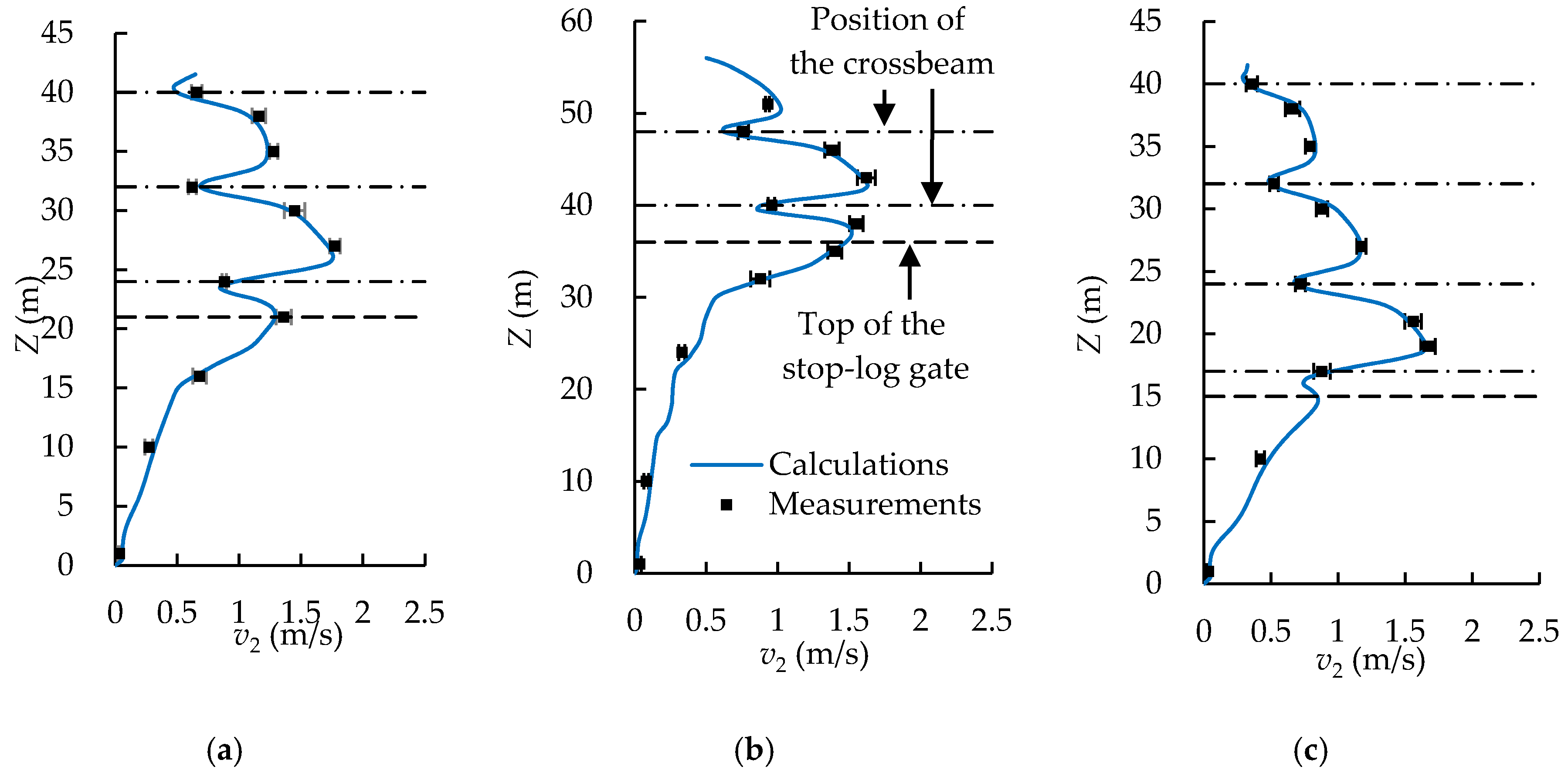
3.1. Comparisons Between Measurements and Simulations

To estimate the model accuracy, the calculated values of v₂ and ΔH are compared with the measured data. Figure 5 shows the comparison of velocity profiles at Section 2 for Cases 3, 8 and 17.

Table 3. Comparison of ΔH between measurements and simulations.

Case	Method	H (m)	p (m)	pv (m)	ΔH (m)	ξ
3	Measurements	42	38.673	1.138	2.189	1.91
	Simulations	42	38.654	1.221	2.125	1.85
8	Measurements	57	53.289	1.210	2.501	2.17
	Simulations	57	53.392	1.277	2.331	2.03
17	Measurements	42	39.121	1.192	1.687	1.47
	Simulations	42	38.998	1.256	1.746	1.52

presents the comparison of ΔH. For v₂, the computed results match well with the measured ones, although there is a certain discrepancy for some points. For ΔH, the calculated results are in compliance with the measured data. The results indicate satisfied model performance for both v and ΔH calculations.

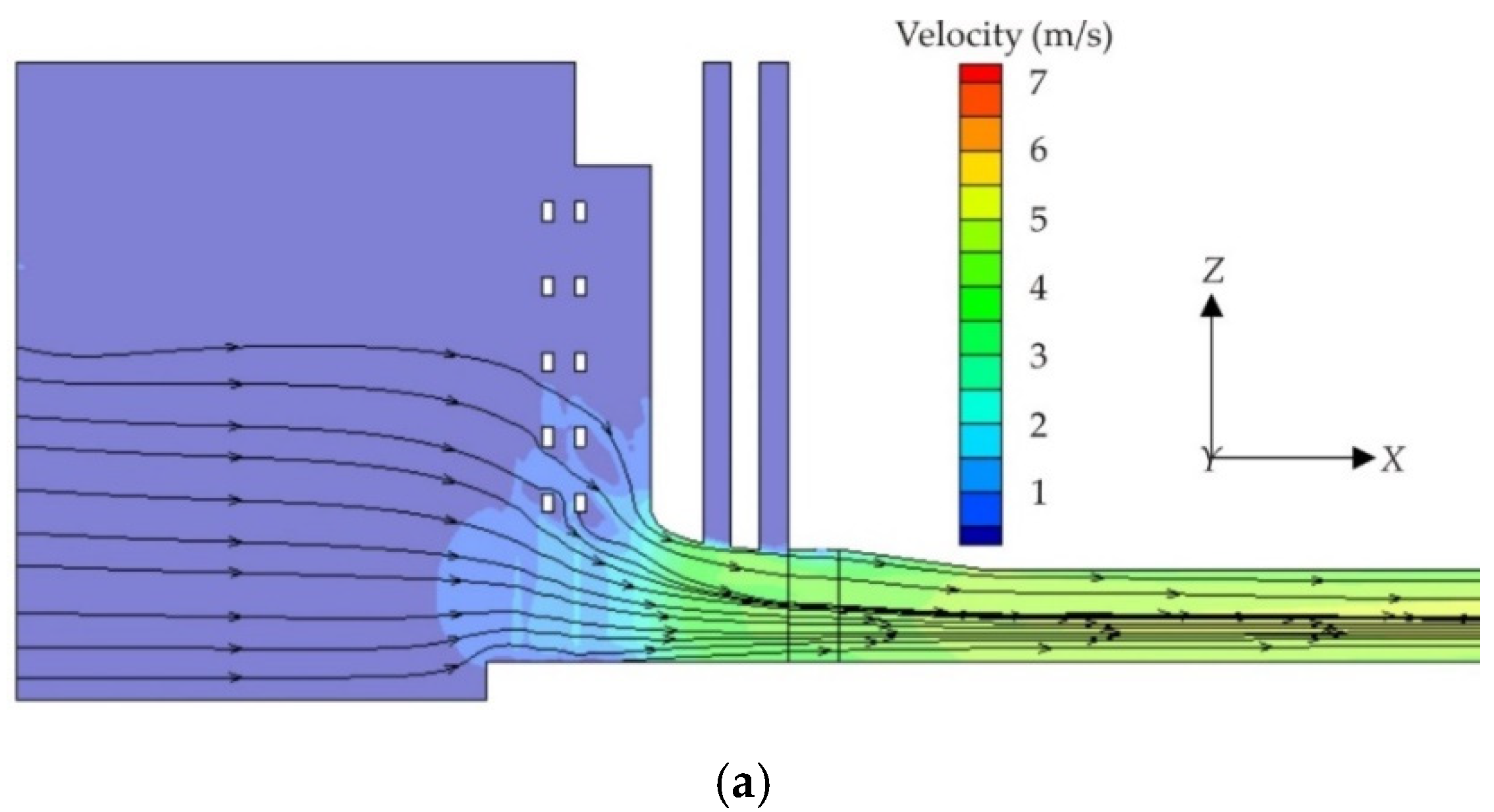
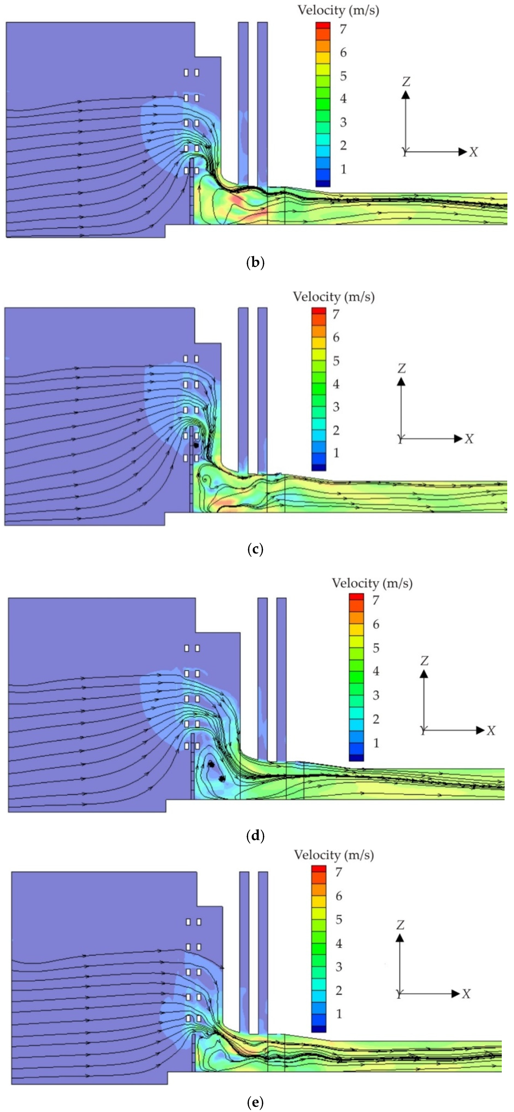
3.2. Flow Regime

The flow behaviors from reservoir running into the water intake are distinct with and without a stop-log gate and exhibit complex features. The flow runs relatively smoothly into the water intake in the absence of the gate (see Figure 6a). From the inlet to its downstream, the velocity shows an augment and reaches the maximum approximately at the Section 3, with the peak value of ~5 m/s. However, it is disadvantaged to withdrawal water at a selective layer. In the presence of a stop-log gate, as shown in Figure 6b–e, the bottom water in the reservoir is blocked to some extent, and the relative up-layer water runs into the intake. This realizes the water withdrawal at a given layer with expected temperature by adjustment of the gate height. To examine the flow features under the variations of H, l and h_s, the longitudinal flow regimes on the X-Z coordinate plane are displayed for selected cases.

In comparison of Case 3 and 5, the effect of H is illustrated in Figure 6b,c; comparing Case 3 and 13 in Figure 6b,d, the effect of l is obtained; to compare the Figure 6b,e, the impact of h_i is demonstrated. The gate acts as a submerged sharp-crested weir, and the inflow bypassing the gate experiences great changes in flow direction. Local head losses occur as the streamlines are directed away from the axial direction of flow due to the changes of the wall geometry, which complies with the study of Hager [35]. Additionally, the flow mixing in the intake chamber also induces some head losses. Looking downwards and behind the gate, a large recirculation zone occurs at the bottom of the intake chamber and a small one is also observed for case 5. The occurrences are attributable to the variations of chamber wall geometry. The recirculation zones reduce the effective inflow area at the location, and thus cause an additional acceleration of the flow. It is believed that recirculation zones are associated with high turbulence phenomena, leading to considerable energy loss [35].

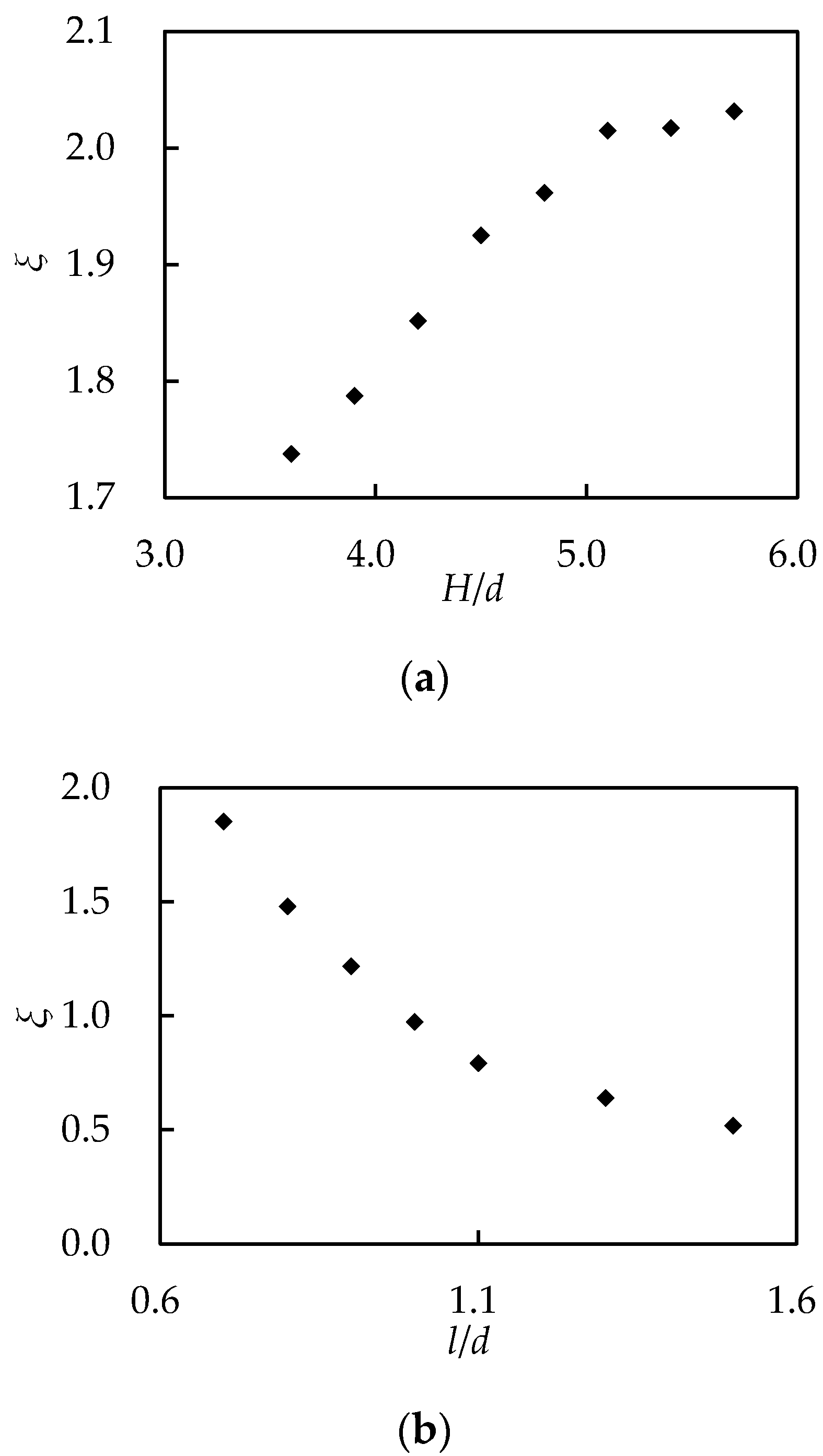
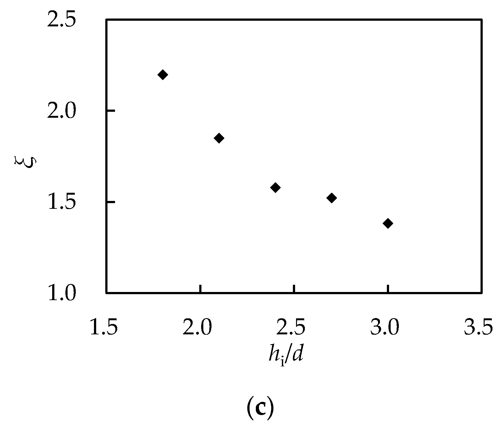
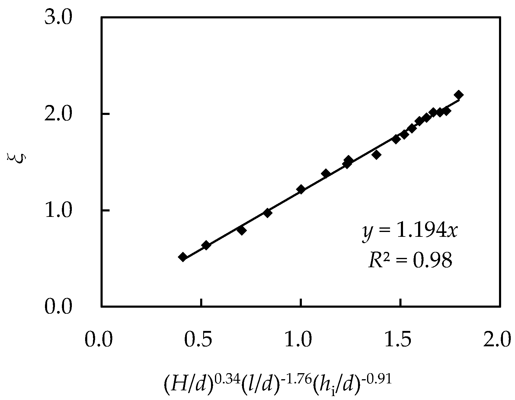
3.3. Head Loss

Head loss is an essential parameter when evaluating the flow running into the intake. As aforementioned, the ξ is a function of H/d, h_i/d and l/d. Figure 7a shows the relationship between ξ and H/d. It is noticed that the ξ augments with the increase of H/d following an approximately linear relationship, which suggests that the increase of the water head in the reservoir leads to a larger head loss at the intake. The result is consistent with previous prototype studies [21]. For a given withdrawal depth h_i, the increase of the water head H means a larger h_s. It contributes to the observations in Figure 7c, where vortices are observed between two crossbeams and the generating turbulent vortices shedding could further develop in the chamber, causing some energy loss.

Figure 7b depicts the relationship between ξ and l/d. It shows that the ξ exhibits a nonlinear decrease trend with the increase of l/d, which is coincident to that obtained by Lei et al. [22]. They report that the relatively large l is recommended in the design of the intake geometry so as to get good flow regime and small head loss. There would be a large flow velocity gradient in the chamber in the situation of small l, contributing to the extensive flow momentum exchange and consequently generating energy dissipation. Moreover, the head loss due to the presence of recirculation zone is greatly affected by the intake geometry. However, the former plays a dominant role. Figure 7c presents the results between ξ and h_i/d. The ξ decreases with the increases of h_i/d, implying that for a given H, a larger h_i corresponds to a smaller h_s, leading to less head loss. To achieve a balance between the least head loss and selective water withdrawal, it is suggested to consider the three parameters simultaneously but not in a separate way.

Based on the measured data, the relationship between ξ and H/d, l/d, h_i/d is derived by means of the multiple regression analysis and reads as

$$\xi =1.194{(\frac{H}{d})}^{0.34}{(\frac{l}{d})}^{-1.76}{(\frac{h_i}{d})}^{-0.91}$$

(8)

Figure 8 shows the plot and R² = 0.98, indicating a good regression.

To verify the derived Equation (8), systematic data from previous studies inclusive of experimental and numerical results are collected for comparison, as listed in

Table 4. Comparison of results between available literature and this study.

Data Sources	H (m)	l (m)	hi (m)	d (m)	Method	ξ		Err (%)
						Previous	Calculated
[20]	89.00	8.00	49	11	exp.	1.15	1.09	5.2
[24]	63.00	12.00	18	8.3	exp.	0.65	0.62	5.1
	45.00	12.00	18	8.3		0.61	0.55	9.8
	33.00	12.00	18	8.3		0.57	0.50	13.1
[25]	61.00	8.00	25	11	exp.	2.06	1.77	14.2
	61.00	8.00	25	11	num.	1.96	1.77	9.8
[26]	14.00	7.00	2	6.4	num.	5.13	4.73	7.9

. Moreover, Figure 9 gives the comparisons between previous (subscript pre) and calculated (subscript cal) results with respect to the ξ. The dotted lines indicate a relative error (Err) of 15% based on the following equation.

$$Err=\frac{\left|{\xi }_{\mathrm{pre}}-{\xi }_{\mathrm{cal}}\right|}{{\xi }_{\mathrm{pre}}}$$

(9)

The multiple correlation coefficients between the previous results ξ_pre and the calculated results ξ_cal are 0.98, and no data scatter >15% on basis of Equation (9), indicating the obtained results agree reasonably well with the previous data. These errors might be ascribed to some different inlet geometries in certain projects.

3.4. Flow Velocity at Trash Rack

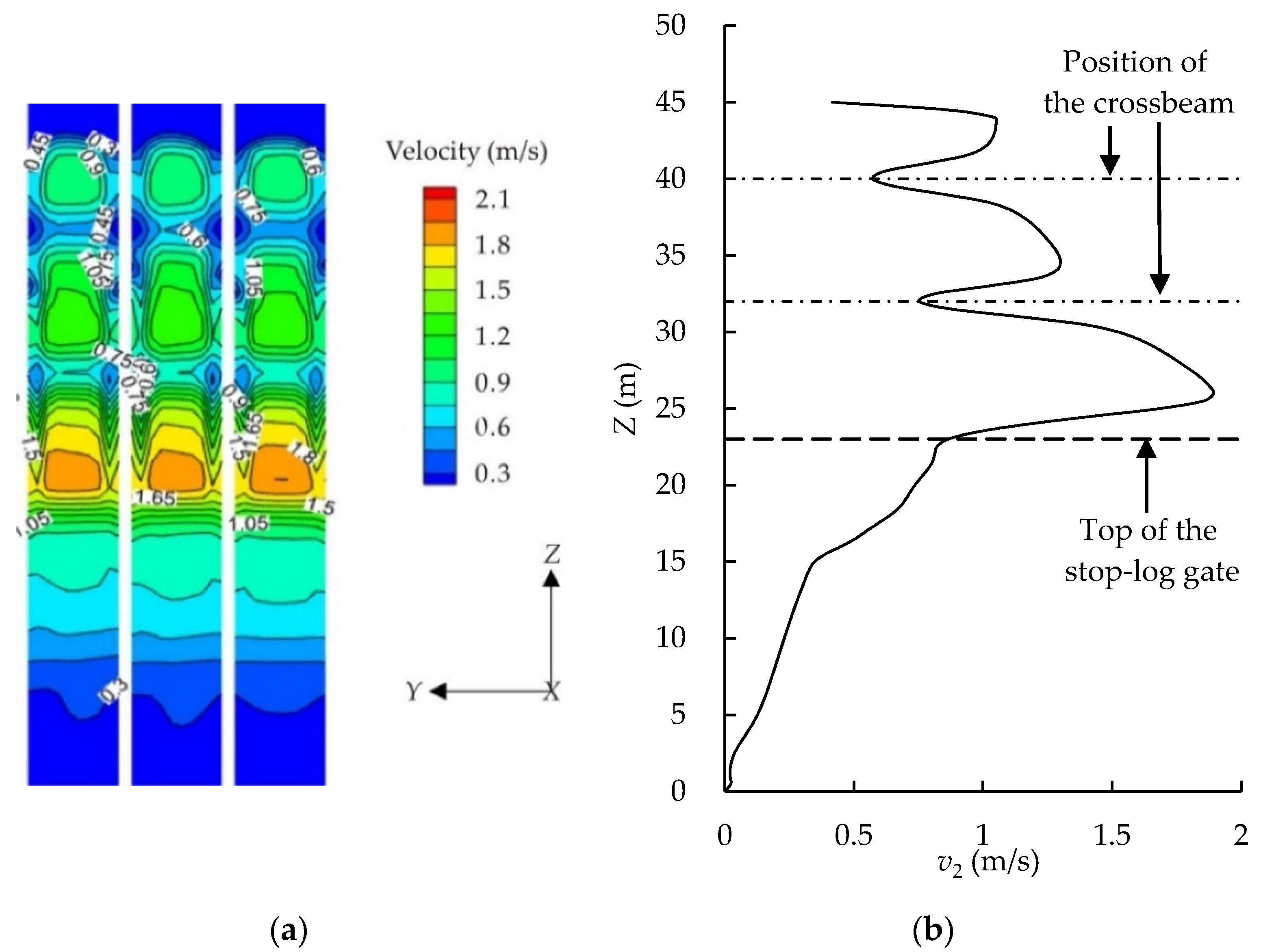
3.4.1. Flow Velocity Distribution

Flow velocity distribution at the trash rack, i.e., Section 2 in Figure 1, is an essential indicator for the structural design, and it is usually characterized by the maximum flow velocity v_2m (m/s) and its position Z_m. To examine the two parameters, Case 4 as an example is chosen for illustration. Figure 10 presents its cross-sectional flow velocity distributions at Section 2.

The flow velocity exhibits a general downward trend from the top of the gate to the water surface. In Figure 10a, it shows that the flow cross-section is divided by the vertical beams into three independent parts, and the velocity distributions in each part are almost identical. The flow velocity is also affected significantly by the presence of horizontal crossbeams. Several different flow regions, as a result, are noticed the cross-section. Figure 10b shows the corresponding flow velocity profile in the vertical direction. The flow velocity is relatively small in the region below the top of stop-log gate, as the flow is blocked by the gate. When the Z increases from Z = 0, flow velocity augments gradually. Once it exceeds the top of the gate, flow velocity surges to the maximum (v_2m = 1.5–1.8 m/s), and then, it decreases. Such flow deceleration is also caused by the horizontal crossbeam. Then similar rebounds in flow velocity exist between two crossbeams till the surface. Considering the structure safety and the racks accessible for cleaning, the v_2m is of great concern in practical and previous experience suggests that v_2m should not be a large value, preferable v_2m ≤ 1.5 m/s, which is also evidenced by Johnson [36].

3.4.2. Maximum Velocity

In light of the flow velocity at the trash rack, it has some relationship with H/d, l/d and h_i/d. To examine the maximum velocity at the trash rack, a dimensionless velocity distribution coefficient K is defined by the v_2m and $\overline{v_2}$ (m/s),

$$K=\frac{v_{2m}}{\overline{v_2}}=\frac{v_{2m}}{Q/A_{2e}}$$

(10)

where $\overline{v_2}$ = the average velocity at Section 2, and A_2e = the corresponding active inflow area.

The relationship between K and H/d is presented in Figure 11a. It is noticed that K fluctuates slightly with the variations of H/d; the data points are scattered in the range of K = 1.6–1.9, with an average value of K = 1.7. Such scattering behavior is the effect of crossbeams on the velocity distribution. As mentioned above in Figure 10, the presence of the crossbeams has a bear on the flow field. Under the different H, the relative vertical position of the crossbeams differs in the section, leading to the difference of flow velocity distributions in Section 2

Similarly, the relationship between K and h_i/d is plotted in Figure 11b. It shows that the K keeps a constant value of 1.7 with different l/d values, implying that the change of width of the intake chamber has little effect on the flow velocity at the trash rack. It is shown in Figure 11c that the K increases from 1.4 to 2.2 with the increase of h_i/d, indicating that the smaller h_i is accompanied with the larger disparity between the v_2m and the $\overline{v_2}$. For a given Q, it is noted that a larger A_2e is exposed to a larger h_i and consequently leading to a smaller $\overline{v_2}$ (v₂ = Q/A_2e). This could contribute to the augments of K with h_i/d. Scattered point is also observed in Figure 11c, which holds the same reason with that of Figure 10a, i.e., the effect of the relative crossbeams positions subjected to different H.

To summarize, in terms of the flow velocity at the trash rack, three parameters, i.e., H/d, l/d and h_i/d, are taken into consideration. The results show that the K is roughly proportional to the h_i/d, exhibiting an increasing trend. It implies that the velocity is affected noticeably by the h_i, also a result of the h_s adjustment.

3.4.3. Position of the Maximum Velocity

The position of the maximum flow velocity Z_m is described by the relative position Z_m/h_s in the present work. The relationship between Z_m/h_s and H/d, l/d, h_i/d is presented in Figure 12. The change of Z_m/h_s with these three parameters is not significant, in spite of some slight fluctuations in Figure 12a,c. Such fluctuations are also ascribed to the changes in flow velocity distribution, induced by the different relative positions of crossbeams in different cases.

It displays that all data points scatter in the range of Z_m/h_s = 1.05–1.30, suggesting that the maximum flow velocity always occurs at a small height above the stop-log gate. Therefore, more attention should be paid to the flow velocity in this range for the design of trash rack structures. The result is consistent with that of the previous study [37], in which a range of Z_m/h_s = 1.05–1.15 is reported. The present work indicates a more extensive range of Z_m/h_s, because more cases with different geometries are taken into account.

4. Conclusions

The research presents an investigation on the hydraulic features of a water intake functioned with a stop-log gate. Considering different flow conditions and geometries, both laboratory experiments and numerical simulations are performed to help understand the intake flow behaviors, including the flow regime, head loss and maximum flow velocity. Simulation results are verified against the experiment data in the present work. The main conclusions are summarized as follows:

(1)

At the water intake, flow regime changes dramatically after the employment of stop-log gate; the occurrence of flow recirculation and vortices in the intake chamber is affected considerably by the water head and the intake geometry.

(2)

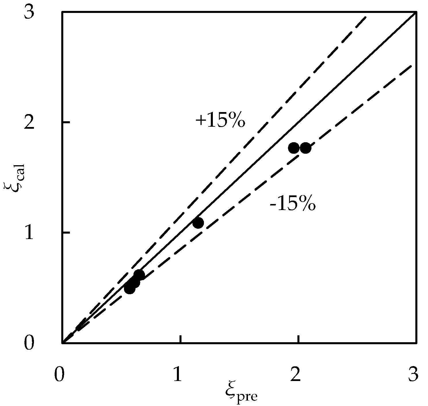
Head loss at the intake depends significantly on the upstream water head, width of intake chamber and withdrawal depth. Based on the regression analysis of systematical data, an empirical equation for the coefficient of head loss is derived; the calculated results from the equation show a good agreement with both experimental and numerical data from previous studies.

(3)

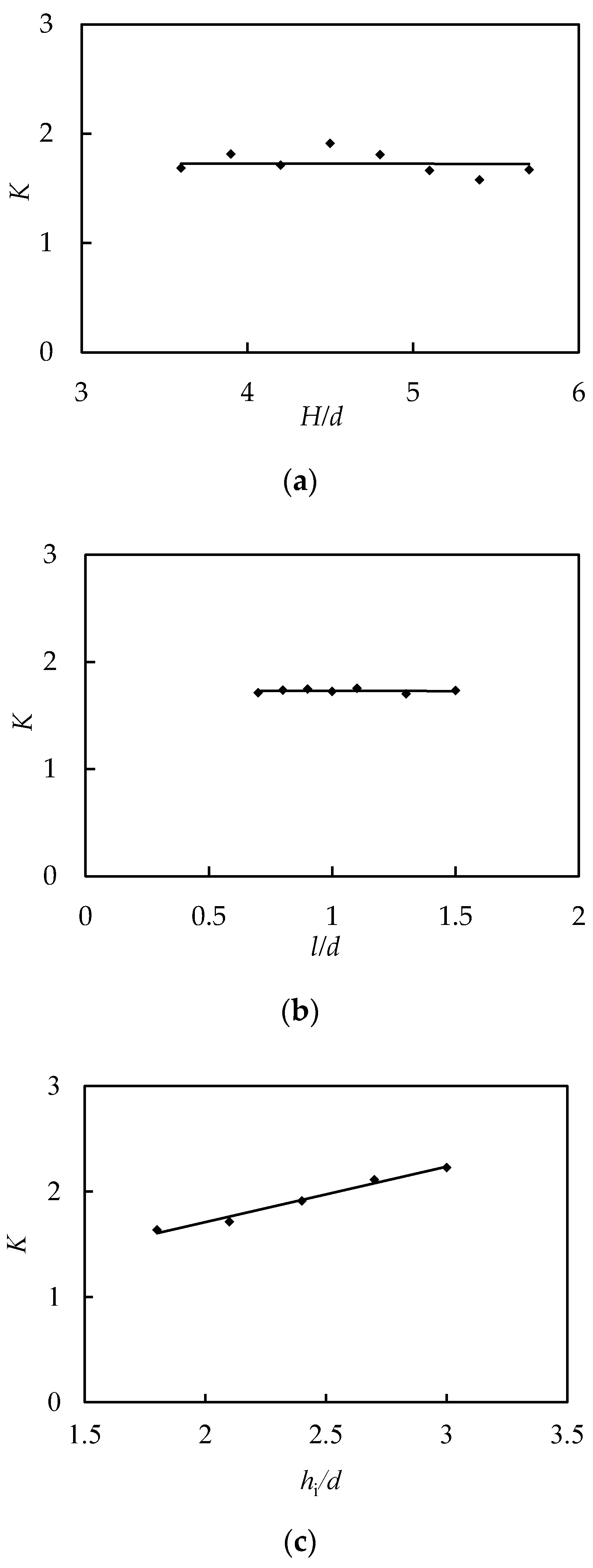
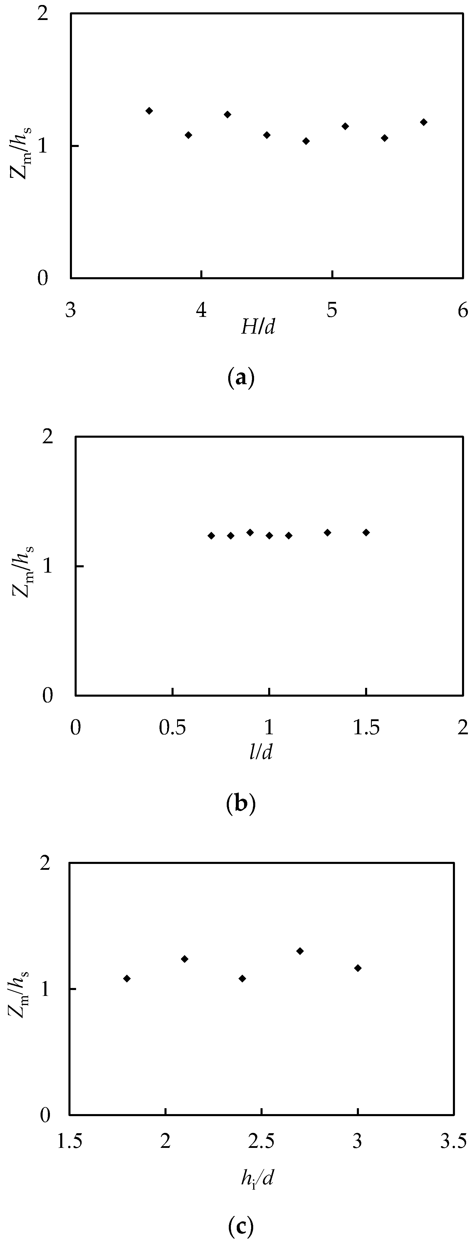
Flow velocity at the trash rack section varies vertically in a great manner. The velocity distribution coefficient is dependent exclusively on the relative intake depth, showing a range of 1.4–2.2 with different depths. Regardless of the different water head and the geometry of stop-log gate, the maximum flow velocity always occurs at roughly 1.05–1.30 times of the gate height.

The combination of the experimental and numerical results reveals the flow behaviors of water intake with stop-log intake, providing general insights into similar hydraulic situations in practice.

References

- Wang, S.; Qian, X.; Han, B.; Luo, L.; Hamilton, D.P. Effects of local climate and hydrological conditions on the thermal regime of a reservoir at Tropic of Cancer, in southern China. Water Res. 2012, 46, 2591–2604. [Google Scholar] [CrossRef]
- Carron, J.C.; Rajaram, H. Impact of variable reservoir releases on management of downstream water temperatures. Water Resour. Res. 2001, 37, 1733–1743. [Google Scholar] [CrossRef]
- Palancar, M.C.; Aragon, J.M.; Sanchez, F.; Gil, R. Effects of warm water inflows on the dispersion of pollutants in small reservoirs. J. Environ. Manag. 2006, 81, 210–222. [Google Scholar] [CrossRef] [PubMed]
- Sherman, B.; Todd, C.R.; Koehn, J.D.; Ryan, T. Modelling the impact and potential mitigation of cold water pollution on Murray cod populations downstream of Hume Dam Australia. River Res. Appl. 2007, 23, 377–389. [Google Scholar] [CrossRef]
- Thorpe, J.E. Life history responses of fishes to culture. J. Fish Boil. 2004, 65, 263–285. [Google Scholar] [CrossRef]
- Lian, J.; Li, P.; He, W.; Shao, N. Experimental and numerical study on the effect of the temperature-control curtain in thermal stratified reservoirs. Appl. Sci. 2019, 9, 5354. [Google Scholar] [CrossRef]
- Zhang, S.; Gao, X. Effects of selective withdrawal on temperature of water released of glen Canyon dam. In Proceedings of the 4th International Conference on Bioinformatics and Biomedical Engineering, Chengdu, China, 18–20 June 2010. [Google Scholar]
- Zheng, T.; Sun, S.; Liu, H.; Xia, Q.; Zong, Q. Optimal control of reservoir release temperature through selective withdrawal intake at hydropower dam. Water Sci. Tech. Water Suply 2017, 17, 279–299. [Google Scholar] [CrossRef][Green Version]
- He, W.; Lian, J.; Yao, Y.; Wu, M.; Ma, C. Modeling the effect of temperature-control curtain on the thermal structure in a deep stratified reservoir. J. Environ. Manag. 2017, 202, 106–116. [Google Scholar] [CrossRef]
- Freckleton, D.R.; Johnson, M.C.; Boyd, M.L.; Mortensen, D.G. Stop logs for emergency spillway gate dewatering. J. Hydraul. Eng. 2011, 137, 644–650. [Google Scholar] [CrossRef]
- Wu, S.; Cao, W.; Wang, H.; Sun, S.; Chen, Q. Research on the multi-level intake water temperature effect of the Yalong River Jinping-I hydropower project. Sci. China Technol. Sci. 2011, 54, 125–132. [Google Scholar] [CrossRef][Green Version]
- Shifei, T. Analysis of the operation of stratified water intake for laminated beam gate of Guangzhao Hydropower Station. Guizhou Water Power 2011, 4, 18–21. [Google Scholar]
- Shamaa, Y.; Zhu, D.Z. Experimental study on selective withdrawal in a two-layer reservoir using a temperature-control curtain. J. Hydraul. Eng. 2010, 136, 234–246. [Google Scholar] [CrossRef]
- Rheinheimer, D.E.; Null, S.E.; Lund, J.R. Optimizing selective withdrawal from reservoirs to manage downstream temperatures with climate warming. J. Water Res. Plan. Manag. 2015, 141, 04014063. [Google Scholar] [CrossRef]
- He, W.; Lian, J.; Liu, F.; Ma, C.; Pan, S. Experimental and numerical study on the thrust of a water-retaining curtain. J. Hydroinform. 2018, 20, 316–331. [Google Scholar] [CrossRef]
- Zhang, L.; Zhang, J.; Peng, Y.; Pan, J.; Peng, Z. Numerical simulation of flow and temperature fields in a deep stratified reservoir using water-separating curtain. Int. J. Envron. Res. Public Health 2019, 16, 5143. [Google Scholar] [CrossRef]
- Vermeyen, T.B. Glen canyon dam multi-level intake structure hydraulic model study. In Water Resources Services, Water Resources Research Laboratory; Technical Service Center: Denver, CO, USA, 1999. [Google Scholar]
- Vermeyen, T.B. An overview of the design concept and hydraulic modeling of the glen canyon dam multi-level intake structure. In Proceedings of the Waterpower 99 Conference, Las Vegas, NV, USA, 6–9 July, 1999. [Google Scholar]
- Zhang, X.; Wang, X. Intake model test for Bakun hydropower project in Malaysiz. Northwest Hydropower 2005, 2, 59–62. [Google Scholar]
- Duan, W.; Huang, G.; Hou, D.; Du, L.; Liu, H. Hydraulic characteristics study on stoplog gates multi-level water intake of large hydropower station. J. Hydroelectr. Eng. 2015, 13, 380–384. [Google Scholar]
- Zhang, J.; Zhang, D.; Wu, Y.; Zhang, W.; You, X. Experimental study on hydraulic characteristics of the stratified intake for the fist-stage Jinping hydropower station. J. Hydroelectr. Eng. 2010, 29, 2–6. [Google Scholar]
- Lei, Y. Research on Numerical Simulation of Turbulent Flow for Stratified Intake in Hydropower Station. Ph.D. Thesis, Wuhan University, Wuhan, China, 2010. [Google Scholar]
- Li, Y.; Gao, X.; Xu, M.; Dong, S.; Zhang, Z.; Liu, X. Study on numerical simulation of hydraulic characteristics of intake for hydropower station. Water Resour. Hydropower Eng. 2010, 41, 29–32. [Google Scholar]
- Peng, X. Numerical Study on Hydraulic Characteristic of Multi-Level Intakes of Hydropower Stations. Ph.D. Thesis, Tianjin University, Tianjin, China, 2013. [Google Scholar]
- Du, L.; Xu, X. Numerical simulation research on the flow field in multi-level intake with stop-log gates of hydropower stations. China Rural Water Hydropower 2013, 8, 158–165. [Google Scholar]
- Zhang, Q. The Hydraulic Characteristics Numerical Simulation Study of Water Intake in the Water Inlet of the Hydropower Station. Master’s Thesis, Hebei University of Engineering, Handan, China, 2018. [Google Scholar]
- ANSYS, Inc. ANSYS Fluent User’s Guide; Release 17.2; ANSYS, Inc.: Southpointe, FL, USA, 2016. [Google Scholar]
- Hirt, C.W.; Nichols, B.D. Volume of fluid (VOF) method for the dynamics of free boundaries. J. Comput. Phys. 1981, 39, 201–225. [Google Scholar] [CrossRef]
- Jothiprakash, V.; Bhosekar, V.; Deolalikar, P.B. Flow characteristics of orifice spillway aerator: Numerical model studies. ISH J. Hydraul. Eng. 2015, 21, 216–230. [Google Scholar] [CrossRef]
- Teng, P.H.; Yang, J.; Pfister, M. Studies of two-phase flow at a chute aerator with experiments and CFD modelling. Model. Simul. Eng. 2016, 2016, 4729128. [Google Scholar] [CrossRef]
- Zhang, J.; Chen, J.; Xu, W. Three-dimensional numerical simulation of aerated flows downstream sudden fall aerator expansion-in a tunnel. J. Hydrodyn. 2011, 23, 71–80. [Google Scholar] [CrossRef]
- Yang, J.; Teng, P.H.; Zhang, H.W. Experiments and CFD modeling of high-velocity two-phase flows in a large chute aerator facility. Eng. Appl. Comput. Fluid Mech. 2019, 13, 48–66. [Google Scholar] [CrossRef]
- Shi, Q.S. High-Velocity Aerated Flow; Water & Power Press: Beijing, China, 2007. [Google Scholar]
- Heller, V. Scale effects in physical hydraulic engineering models. J. Hydraul. Res. 2011, 49, 293–306. [Google Scholar] [CrossRef]
- Hager, W.H. Wastewater Hydraulics: Theory and Practice, 2nd ed.; Springer: Berlin, Germany, 2010; pp. 29–33. [Google Scholar]
- Johnson, P.L. Hydro-power intake design considerations. J. Hydraul. Eng. 1998, 114, 651–661. [Google Scholar] [CrossRef]
- Liu, H.; Sun, S.; Zheng, T.; Li, G. Analysis on velocity distribution characteristics of trash rack for intake with stoplog gate of large-sized hydropower station. Water Resour. Hydropower Eng. 2018, 49, 89–96. [Google Scholar]