Comparing Trends in Modeled and Observed Streamflows at Minimally Altered Basins in the United States

Abstract

We compared modeled and observed streamflow trends from 1984 to 2016 using five statistical transfer models and one deterministic, distributed-parameter, process-based model, for 26 flow metrics at 502 basins in the United States that are minimally influenced by development. We also looked at a measure of overall model fit and average bias. A higher percentage of basins, for all models, had relatively low trend differences between modeled and observed mean/median flows than for very high or low flows such as the annual 1-day high and 7-day low flows. Mean-flow metrics also had the largest percentage of basins with relatively good overall model fit and low bias. The five statistical transfer models performed better at more basins than the process-based model. The overall model fit for all models, for mean and/or high flows, was correlated with one or more measures of basin precipitation or aridity. Our study and previous studies generally observed good model performance for high flows up to 90th or 95th percentile flows. However, we found model performance was substantially worse for more extreme flows, including 99th percentile and annual 1-day high flows, indicating the importance of including more extreme high flows in analyses of model performance.

1. Introduction

Daily streamflow records are important for effective management of water resources for rivers, streams, and reservoirs [1]. Flows of interest to managers such as flood flows (e.g., Arneson et al. [2]) and 7-day low flows (e.g., U.S. Environmental Protection Agency [3]) can be determined from the daily values. Changing flows over time are also important to water management, as climatic changes and basin development can increase or decrease flows (e.g., Hodgkins et al., Dudley et al., Vincente-Serrano [4,5,6]). In the United States, streamflow trends have varied by region during the last century. There have been increases in peak flows for many basins in the Northeast and Midwest and many decreases in the West and South [4]. For low flows, there have been many increases in the Northeast and Midwest and many decreases in the Southeast [5].

Only a limited number of streamflow gages are feasible in any given country, and there are many spatial and temporal gaps in observed streamflow records (e.g., Kiang et al. [7]). Therefore, methods to estimate daily flows are needed, and evaluation of models against observational data is crucial [8]. Models are commonly evaluated against long-term mean annual or monthly values for large basins. Relatively few studies have evaluated large-domain models for high and low streamflows [9]. It is important to evaluate models for small to medium sized basins and for multiple flow metrics to better understand rainfall–runoff processes and streamflows across a range of scales.

The U.S. Geological Survey (USGS) has developed a large-domain model infrastructure to characterize basin variables and parameters such as soil moisture, vegetation, snow dynamics, climate, evapotranspiration, contributing area, and topography and to estimate daily streamflow across the United States [10]. This National Hydrologic Model infrastructure (NHM) allows for process-based, distributed modeling that can provide information for ungaged basins. While the NHM could be adapted for use with many hydrologic simulation models, the current (2020) NHM uses the USGS Precipitation-Runoff Modeling System (PRMS) [11,12,13] to compute daily streamflows.

It is also possible to estimate flows at ungaged basins using statistical transfer models. These models include ones based on drainage-area ratios [14] and ones based on nonlinear spatial interpolation using flow duration curves (QPPQ) [1,15]; they require flows from an index gage to transfer flow information to ungaged locations. The index gage for these methods can be determined with both a nearest neighbor approach (minimum distance to an index gage) or by map correlation (maximum estimated correlation) [1,16]. Another approach is to use multiple index sites with weights determined by pooled ordinary kriging [17].

An important component of large-domain modeling is evaluating how well the models reproduce daily flows, flow metrics, and trends. Large-domain comparisons of predicted and observed flow metrics are limited, particularly with respect to models reproducing observed trends. Stahl et al. [8] compared modeled and observed flows, including trends, for a large number of small near-natural basins in Europe from 1961–2004, for a high-resolution regional climate-model simulation. They found that temporal trends agreed well for trends toward drier conditions about half the time; for trends toward wetter conditions, they agreed about two-thirds of the time. Gudmundsson et al. [9] compared an ensemble of nine hydrologic models to observed aggregated data from 426 small near-natural basins in Europe. Models were evaluated on how well they captured the magnitude and interannual variability of five flow percentiles, from low to high flows. Alkama et al. [18] compared monthly modeled flows from a process-based hydrologic model to observed monthly-flow trends for 154 large basins worldwide from 1960 to 1994. In the U.S., Lohmann et al. [19] compared 3 years of modeled to observed flows for four hydrologic models at 1145 small and medium basins gaged by the USGS, for daily, monthly, and annual time steps.

Farmer et al. [1] conducted a pilot study in the Southeast U.S. of 182 near-natural basins over a 30-year period to determine advantages and limitations of both process-based and statistical models for estimating daily streamflow and streamflow metrics in ungaged basins. Farmer [17] compared the performance of several statistical transfer models against aggregated observed flows (low to high) from the same basins, including ordinary kriging, drainage-area ratio, and non-linear spatial interpolation using flow duration curves (QPPQ).

Multiple evaluation studies are currently (2020) underway to evaluate the U.S. National Hydrologic Model; this article focuses on evaluation of trend reproduction in the conterminous U.S. for five statistical models and one process-based model, for 502 basins that are minimally influenced by basin development. To provide context for trend reproduction, we also evaluate overall model fit and bias.

2. Data and Methods

2.1. Observed Data

Observed daily streamflow data from water year 1984 (beginning 1 October 1983) through water year 2016 (ending 30 September 2016) were downloaded from the USGS National Water Information System [20] for all Hydro-Climatic Data Network 2009 streamflow gages [21] in the conterminous United States. Basins with this designation are considered to be relatively free from human disturbance or alteration and are therefore affected mainly by climatic changes and variability [22]. These data were downloaded using the R package “dataRetrieval” [23,24], screened for “approved” status, and subjected to length and completeness testing. Streamflow records were expected to have a daily value for every day of the water year (denoting a complete water year) for at least 8 out of every 10 years in each decade (e.g., 1990–1999) for the study period (water years 1984–2016). Partial decadal periods of 1984–1989 and 2010–2016 were required to have 5 of 6, and 6 of 7 complete years, respectively. Application of these data length and completeness criteria yielded 613 Hydro-Climatic Data Network 2009 gages with adequate streamflow record.

As explained below, 502 of these 613 gages were used for comparisons between modeled and observed flows. These 502 gages drain basins across the conterminous United States (Figure 1) with higher densities of gaged basins in parts of the eastern half of the U.S. and on the West Coast. Basins have a median area of 379 km² (5th percentile: 30.4 km², 95th percentile: 2910 km²) [21], median annual basin precipitation of 1110 mm (508 mm, 2430 mm), median annual potential evapotranspiration of 649 mm (390 mm, 1020 mm), and median annual air temperature of 10.2 °C (2.0 °C, 19.0 °C). As mentioned above, the basins are considered minimally altered but this includes substantial agricultural area in parts of the U.S. as Hydro-Climatic Data Network 2009 basins are considered minimally altered on a regional basis. Basins contain a median crop area of 0.31% (0.0%, 59.8%), a median urban area of 3.6% (0.0%, 7.5%), and a median forested area of 60.6% (0.9%, 91.6%). Gages used in this study, observed streamflow data, and basin metadata are available in [25].

2.2. Data from a Process-Based Model

The National Hydrologic Model Infrastructure application of the Precipitation-Runoff Modeling System (NHM-PRMS) [10,11,12,13,26] was used to simulate daily streamflow at all gaged locations in this study from 1 October 1983 to 30 September 2016. The data are available in a USGS data release [27]. The NHM-PRMS is a deterministic, distributed-parameter, process-based model that simulates the effects of precipitation, air temperature, and land use on basin hydrology. It uses the Geospatial Fabric for National Hydrologic Modeling [28] with Hydrologic Response Units and a stream network for the conterminous U.S. The hydrologic response units have a median size of 33.2 km².

Daily values of observed precipitation and maximum and minimum air temperature from the Daily Surface Weather and Climatological Summaries version 3 [29,30,31] were used for each hydrologic response unit to compute potential evapotranspiration, actual evapotranspiration, sublimation, snowmelt, streamflow, infiltration, and groundwater recharge [11]. Physical characteristics used include topography, soils, vegetation, geology, and land cover. Effects of water use and flow regulation were not modeled.

A stream network was used to route hydrologic-response-unit-based surface runoff, shallow subsurface runoff, and groundwater flow downstream to the basin outlets used in the current study. Muskingum routing was used for channel routing computations. Modeled flows were provided for each stream segment that was collocated with each study stream gage. A linear drainage-area-ratio correction was applied to simulated streamflows for all basins for which the Geospatial Fabric drainage area differed from published National Water Information System drainage areas by <15 percent. Simulated streamflow results from basins for which National Hydrologic Model and National Water Information System drainage areas differed by ≥15 percent were not used.

Static model parameterization was completed for each basin in the current study as described in Lafontaine [11] for physical characteristics, initial water content, and climate. Models were calibrated in two steps referred to as: (1) “by-hydrologic-response-unit” and (2) “by-headwater” [11]. In the first step, each of the model hydrologic response units were calibrated individually. In the second step, headwater subbasins (collections of hydrologic response units and stream segments) that were 3000 square kilometers or smaller were calibrated [11]. Measured streamflow was used in these two calibration steps but in an indirect manner, as described below. The “by-hydrologic-response-unit” calibration focused on water volume optimization for several parts of the hydrologic cycle, and the “by-headwater” calibration focused mainly on streamflow volume and timing optimization. For the “by-hydrologic-response-unit” calibration, the hydrologic simulation for each hydrologic response unit in the conterminous U.S. was calibrated to monthly values of runoff, actual evapotranspiration, and snow-water equivalent (see Lafontaine [11] for details). The calibration datasets were obtained from a combination of existing modeling applications and remotely sensed datasets. Runoff calibration targets were computed from the Monthly Water Balance Model [32], which was calibrated to measured streamflow. Monthly actual evapotranspiration was derived from the Monthly Water Balance Model, the MOD16 global evapotranspiration product [33], and the Simplified Surface Energy Balance model [34]. Monthly snow-water equivalent was derived from the Monthly Water Balance Model and the SNODAS dataset [35]. For the “by-headwater” calibration, headwater subbasins were used in a five-step calibration procedure that included the results from the “by-hydrologic-response-unit” calibration to optimize the match between PRMS-derived streamflows at the headwater subbasin outlets and statistically derived streamflow simulations constructed using an application of ordinary kriging developed by Farmer [17]. The headwater subbasin drainage area limit was chosen as an upper limit for identifying basins with an approximate instream travel time of one day. Streamflow calibration metrics used in this step included streamflow volume, timing and magnitude of high-flow days, and timing and magnitude of low-flow days (see Lafontaine [11] for details). The ordinary-kriging based streamflow simulations used at this stage were developed using measured streamflow in a leave-one-out validation framework and were used for their timing information at a daily time step. The typical third calibration step for NHM-PRMS, “by-observations”, that calibrates directly to observed streamflows at basins of interest, was not used because the objective of the current study is to compare modeled against observed streamflows.

2.3. Data from Statistical Transfer Models

Five statistical transfer models were used to simulate daily streamflow at all gaged locations in this study from 1 October 1980 through 30 September 2017. The five models were nearest-neighbor drainage area ratio (NNDAR), map-correlation drainage area ratio (MCDAR), nearest-neighbor nonlinear spatial interpolation using flow duration curves (NNQPPQ), map-correlation nonlinear spatial interpolation using flow duration curves (MCQPPQ), and ordinary kriging of the logarithms of discharge per unit area (OKDAR). The statistically modeled data are available in a USGS data release [36].

NNDAR, MCDAR, NNQPPQ, and MCQPPQ estimates were computed following methods described by [1] with updates to the flow-duration curve modeling which is described in [37]. OKDAR estimates were computed following methods in [17]. Daily streamflow estimation was conducted in a leave-one-out-cross-validation approach where each streamgage was treated as if ungaged and all the remaining streamgages in a study region (hydrologic unit code level-2 regions as defined by Falcone [21]) were used to calibrate each method and perform estimations at the “ungaged” locations.

The statistical transfer models that use nearest-neighbor (NN) or map correlation (MC) use a single index gage to transfer information to the “ungaged” locations in the current study. The NN approach uses the smallest Euclidean distance between sites. The MC approach [16] uses ordinary kriging to select the index gage. Additional details of the MC approach can be found in [1] and [16]. The ordinary-kriging (OK) method [17] uses pooled ordinary kriging of the logarithms of discharge per unit area (OKDAR) to weight multiple index sites for use in estimating streamflows at “ungaged” locations.

The drainage-area-ratio (DAR) method [14] assumes that the streamflow per unit basin area is the same between the index site(s) and the “ungaged” location. Flows are transferred between sites using the ratio of the drainage areas of the two sites. The QPPQ method assumes that the exceedance probability of streamflow on a given day is the same between the index site and the “ungaged” site. The flow on a given day at the index site is converted to an exceedance probability, this exceedance probability is transferred to the “ungaged” site and then converted to flow. The exceedance probabilities for the “ungaged” sites were computed with regional multiple-linear regression (see Farmer et al. [1] for details).

For the current study, streamflows from the five statistical models and the process-based model NHM-PRMS were compared with observed flows from 1 October 1983 through 30 September 2016 which is the period of overlap for all the modeled data. Overlap between Hydro-Climatic Data Network 2009 gages meeting data length and completeness criteria described above with available PRMS and statistical model gages yielded 502 study gages in common to all.

2.4. Methods

A suite of 26 streamflow metrics was derived from the observed and all six modeled time series (one process-based model and five statistical-transfer models) at all study gages, yielding annual time series for subsequent analyses. All metrics were derived from daily mean flows for complete years on a water year basis (beginning 1 October and ending 30 September and named for the year in which it ends) except for the 7-day low-streamflow metric, which was computed on a climatic year basis (beginning 1 April and ending 31 March and named for the year in which it ends). The streamflow metrics were the annual mean, annual 1-day and 3-day maximums, annual 7-day minimum, a range of annual flow percentiles (1st, 5th, 10th, 25th, 50th, 75th, 90th, 95th, and 99th) and mean monthly flows.

A subset of snowmelt-dominated study gages was identified from the set of gages used by [38,39]. Selection criteria for study gages in Dudley et al. [39] required Hydro-Climatic Data Network 2009 designation, an average of 30 percent or more of total precipitation to fall as snow during the period 1901–2000, and each streamflow record was required to meet 80-percent decadal completeness. Study gages for the current study that overlapped with those identified in Dudley et al. [39] were designated as snowmelt-dominated gages (n = 62) and analyzed for a streamflow metric that represents the overall annual timing of snowmelt-related runoff—the winter-spring center-volume date. This metric was computed as the Julian date when half of the total seasonal runoff volume is equaled or exceeded. The seasonal runoff period was 1 January to 31 July for gages west of 95 degrees west longitude and 1 January to 31 May for gages east of 95 degrees west longitude.

The annual time series analyzed were audited for the frequency of zero-flow values. Time series (observed or modeled) for any metric that had 11 or more (out of 33) years of zero-flow values were flagged as being a “zero-flow” basin-metric combination. The “zero-flow” status was used to guide trend testing methods, as described below.

Trend tests were completed using Sen’s slope [40] for magnitude, except in cases when the annual series had “zero-flow” status for any observed or modeled time series for a given basin; in those cases, the time series was converted to a binomial series, and a logistic regression [41] was done with year as the explanatory variable. The predicted probabilities from the model (dependent variable) were used to quantify the change in probability of a zero-flow year over time. Sen’s slope was computed using the R function “GeneralMannKendall.R”; the function is authored by Benjamin Renard of Irstea, UR Riverly, Lyon, France and is available for download from Dudley et al. [42]. Logistic regression was completed using the “glm” function in the R “stats” package with family = binomial (link = “logit”). Correlations between basin characteristics for study basins and project results were computed with Kendall’s tau.

Two simple evaluation metrics, volumetric efficiency (VE) and average percent bias, were computed to quantify the agreement between observed and modeled annual flow metrics for each basin, such as 1-day maximum flows, mean flows, and 7-day low flows. The volumetric efficiency (VE) [43] was computed as an overall goodness-of-fit metric:

$$VE=1-\frac{{\sum }^{}|Q_{modeled}-Q_{observed}|}{{\sum }^{}{Q}_{observed}}$$

(1)

where a value of 1 indicates a perfect match. Average percent bias at each basin was computed as the sum of the difference between modeled and observed values for each year (the sum of residuals), divided by the sum of the observed values and converted to percent. Volumetric efficiency and average percent bias were computed using the “VE” and “pbias” functions, respectively, in the “hydroGOF” R package [44]. For zero-flow basin-metric combinations, average bias was computed as the difference between the modeled and observed number of years that a streamflow metric (such as 7-day low flows) had zero flow.

3. Results

3.1. Overall Streamflow Metric Comparisons

We compared modeled streamflow trends from 1984 to 2016 to observed trends for various annual flow metrics. Observed positive and negative trends greater than 25% for this period are present at many basins in the conterminous U.S., for mean flows, 7-day low flows, and 1-day high flows (Figure S1). The direction of trends is consistent in some regions, including decreases in mean flows at many basins in the Southwest and increases in the Midwest, decreases in 1-day high flows in the Southwest, and increases in 7-day low flows in the Northeast and decreases in the Southeast. Overall differences in trends were based on results from hundreds of diverse but minimally altered basins across the conterminous U.S. Trends were compared between metrics (13 annual-flow metrics, a measure of snowmelt-related streamflow timing, and monthly mean flows) and between six models (five statistical transfer-based models and one process-based model). Trend analyses were handled separately for flow metrics at basin-metric combinations with a substantial number of zero-flow years. In addition to trend comparisons, we compared modeled and observed streamflow metrics using a measure of model fit, volumetric efficiency, and also with a measure of bias (average percent bias).

Overall, high and low streamflows were modeled poorly compared to mean or median flows when analyzing trend differences between modeled and observed flows, overall model fit, and model bias. All six models analyzed in this study show a higher percentage of basins in the U.S. with relatively low trend differences for annual mean flows, compared to 1-day high flows or 7-day low flows (Figure 2). The brown shades in Figure 2 represent the percent of basins with model-trend underpredictions for 3 increasingly large trend-difference categories while the blue colors represent model overpredictions. Trend underpredictions indicate that the model predicted either (1) smaller positive trends than observed or (2) predicted negative trends when the observed trends were positive.

Differences between modeled and observed trends depend to some degree on the magnitude of observed trends. There were significant negative relations between trend differences and observed trends for basins in this study (

Table 1. Correlations between (1) the magnitude of the difference between modeled and observed trends and (2) the magnitude of observed trends for six models.

Model	Kendall’s Tau			p-Value
	7-Day Low	Mean	1-Day High	7-Day Low	Mean	1-Day High
NNDAR	−0.17	−0.20	−0.22	1.25 × 10−6	4.65 × 10−11	1.23 × 10−13
MCDAR	−0.28	−0.21	−0.27	3.24 × 10−16	1.09 × 10−12	3.22 × 10−19
NNQPPQ	−0.26	−0.30	−0.31	3.65 × 10−14	2.32 × 10−23	1.33 × 10−24
MCQPPQ	−0.37	−0.34	−0.37	4.83 × 10−28	4.77 × 10−30	5.26 × 10−35
OKDAR	−0.30	−0.22	−0.25	3.38 × 10−18	6.24 × 10−14	2.08 × 10−17
NHM-PRMS	−0.33	−0.27	−0.28	4.33 × 10−22	2.40 × 10−19	6.37 × 10−21

), though the magnitudes of many of the correlations were relatively weak. Larger trend underpredictions are related to larger positive observed trends at basins, and larger trend overpredictions are related to larger negative observed trends. In other words, on average, models did not predict wet enough trends or dry enough trends. This relation was strongest for the MCQPPQ model and weakest for the NNDAR model. The negative relations between trend differences and observed trends are seen for 7-day low flows, mean flows, and 1-day high flows.

The largest percentage of basins with relatively good overall model fit (volumetric efficiency, Figure 3, bright green shade) were also for mean flows rather than high or low flows. The same is true for model bias (Figure 4); brown shades in Figure 4 represent negative model bias (modeled flows of lower magnitude than observed flows), and blue shades indicate positive bias.

Results from a more comprehensive set of flow metrics (Supplemental Tables S1–S6 with annual 1st, 5th, 10th, 25th, 50th, 75th, 90th, 95th, and 99th percentile flows, plus 3-day high flows for the six study models) are consistent with the 7-day low, mean, and 1-day high flow results described above.

The winter-spring center-volume date is a measure of the timing of snowmelt-related runoff; it was computed at the snowmelt-dominated basins shown in Figure 5. Upward-pointing triangles indicate trends toward later dates and downward-pointing ones indicate trends toward earlier dates. Blue-shaded symbols indicate that models predicted a later date than was observed while brown-shaded symbols indicate earlier modeled dates than observed. All models do a very good job simulating this metric with almost all basins in the highest volumetric efficiency category (Supplemental Tables S1–S6); however, all models have more basins with 1- to 3-day trend underpredictions than 1- to 3-day overpredictions. In other words, the models predict earlier snowmelt-related runoff than observed for many basins. For monthly mean flows, some months were modeled better than others (Supplementary Tables S1–S6); however, this may be due to typical flow amounts in various months. For example, all models have few basins in the best volumetric efficiency category for July, August, or September mean streamflows, and these months typically have lower flows than winter and spring months.

3.2. Comparisons between Models

NHM-PRMS, the only process-based model in the study, modeled observed flow trends well at fewer basins than the statistical transfer models for low, mean, and high flows (Figure 2). NHM-PRMS overestimated temporal trends for many basins for all flow levels. NHM-PRMS also had fewer basins with high volumetric efficiency (Figure 3) and low bias (Figure 4). It had a relatively high percentage of snowmelt-dominated basins (35.5%) with large trend underpredictions for snowmelt-related streamflow timing and the highest percentage of basins with small negative biases (winter-spring center-volume date, Supplementary Table S6). NHM-PRMS often predicted earlier snowmelt-related runoff timing over time in the western U.S. where the observed trends generally did not show a trend (Figure 5).

The differences between modeled temporal trends and observed temporal trends vary among the statistical transfer models. MCQPPQ, NNQPPQ, and OKDAR had the highest percentage of basins with low trend differences for mean and high flows while NNQPPQ did best for low flows compared to the other statistical transfer models (Figure 2, Supplemental Tables S1–S5). The statistical transfer models had a similar percentage of basins with overpredicted trends as underpredicted trends for all flow levels.

NNDAR and MCDAR had the highest percentage of basins with low model bias for mean flows (Figure 4). For NNDAR, MCDAR, NNQPPQ, and MCQPPQ, more basins had low model bias for high flows than for low flows. For OKDAR the situation was reversed, with a low percentage of basins having low model bias for high flows. OKDAR and PRMS had many basins with a negative bias for high and mean flows. NNQPPQ and MCQPPQ had more basins with negative bias than positive bias for low and mean flows and NNDAR and MCDAR had slightly more basins with positive bias for high and mean flows.

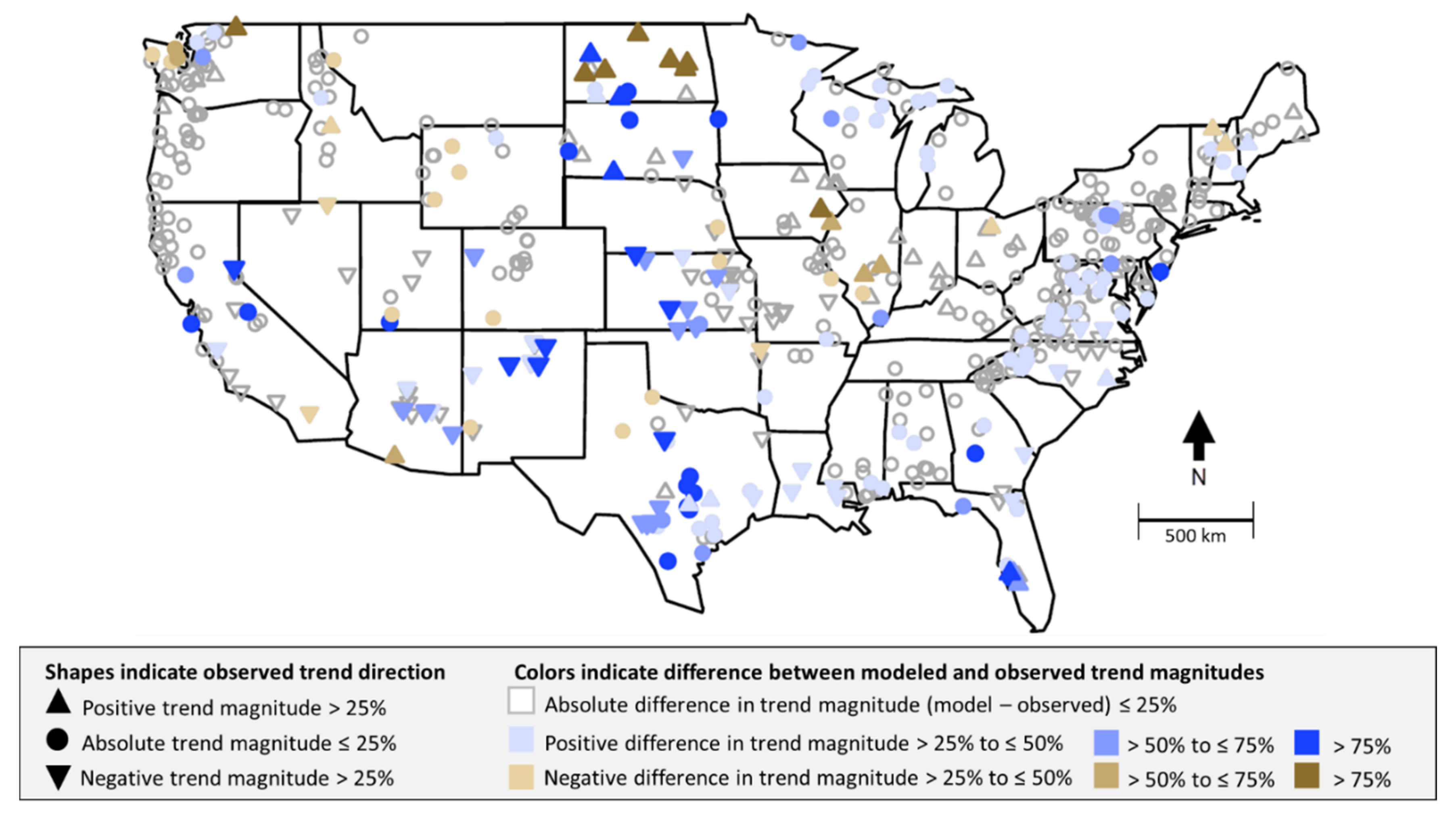
3.3. Geographic Distribution of Results

The geographic distribution of differences between modeled and observed trends, overall model fit (volumetric efficiency), and average bias are shown in Supplemental Figures S1–S6 (one supplemental figure per model with three maps each for 1-day high flows, mean flows, and 7-day low flows). A set of example maps is shown in Figure 6 for NNQPPQ mean flows. For the six models, for mean flows, large trend differences, low volumetric efficiency, and high bias were generally much more numerous in the western half of the conterminous U.S. than the eastern half (Figure 6 and Figures S1–S6). This may be caused by mean flows in arid or semi-arid areas being lower magnitude and less predictable than in more humid areas. More large trend differences and low volumetric efficiencies were seen for 1-day high flows (Figures S1–S6) for NNQPPQ and OKDAR in the western half of the U.S. More basins with high model bias were seen for MCDAR, OKDAR, and PRMS in the western half of the U.S. No obvious geographic patterns were seen for 7-day low flows (Figures S1–S6). The only obvious pattern for snowmelt-related streamflow timing (winter-spring center-volume date) was seen for NHM-PRMS, where modeled trends were overpredicted at some basins in the northeastern U.S. and underpredicted at many basins in the western U.S. (Figure 5).

3.4. Correlations with Basin Characteristics

We correlated trend differences between modeled and observed flows, overall model fit (volumetric efficiency), and average bias for each basin with 77 basin characteristics from the Geospatial Attributes of Gages for Evaluating Streamflow II database [21], for an initial look at which basin characteristics were important to model performance. These characteristics included basin location; physical basin characteristics such as area, elevation, and slope; basin-alteration characteristics such as reservoir storage, developed area, and groundwater withdrawals; basin climatic metrics such as temperature, precipitation, and snow (percent of annual snow to precipitation); average baseflow indices; and soil types. We computed the unitless annual aridity index by dividing the Geospatial Attributes of Gages for Evaluating Streamflow II potential evapotranspiration variable (computed from the Hamon equation) by the precipitation variable PPTAVE_BASIN (30-year average) [21].

There were many significant correlations between study results and basin characteristics but most had weak Kendall’s tau values (t < 0.3). There were no strong (t > 0.3) correlations between trend differences and any basin characteristics. The volumetric efficiency for all six study models, for mean and/or high flows, had a strong correlation with one or more basin precipitation or aridity metric. In addition, some models showed strong correlation with basin longitude, consistent with the mapped results above. All strong correlations were significant at p < 0.0001. All correlations with measures of basin precipitation were positive and measures of aridity were negative; models performed better in wetter basins. WD_BASIN, WDMIN_BASIN, and WDMAX_BASIN are 30-year average metrics representing the annual number of days of measurable basin precipitation, monthly minimum days, and monthly maximum days, respectively [21]. NNDAR had strong positive correlation with WDMIN_BASIN for mean flows; NNQPPQ with WD_BASIN (positive correlation) and basin aridity (negative correlation) for 1-day high flows; MCDAR with WD_BASIN and WDMIN_BASIN for mean and high flows, and aridity for high flows; MCQPPQ with WD_BASIN and aridity for mean and high flows; OKDAR with WD_BASIN and WDMIN_BASIN for mean and high flows and also with WDMAX_BASIN and aridity for high flows; and PRMS with WD_BASIN, WDMAX_BASIN, and aridity for mean and high flows and with WDMIN_BASIN for mean flows. NNDAR, MCDAR, and OKDAR had strong correlations with basin longitude for mean flows.

3.5. Streamflow Metric and Model Comparisons for Variables at Basins with a Substantial Number of Years with Zero Flows

Basin-metric combinations that had 11 or more years of modeled or observed zero flows in the 33-year study period (called “zero-flow basins”) were analyzed separately from basins that did not meet this criterion. The “zero-flow” condition occurred most frequently for low-flow metrics such as the 7-day low flow; we report results only from this metric. Logistic regression was used to analyze temporal trends in the probability of zero-flow years. Trends were then compared between modeled and observed values. Model bias for basin streamflow metrics was computed as the difference between the modeled and observed number of years of zero flow. Model-trend overpredictions represent trends toward more zero-flow days than observed and thus predict trends toward drier conditions than observed; also, model-bias overpredictions represent more years with zero flows, and thus models predicting drier conditions than observed.

Modeled trends were poor for a large percentage of basins (Figure 7). Zero flows for 7-day low flows represent extreme low-flow conditions. Models overpredict (brown-shaded area in the bar charts) or underpredict trends (blue-shaded area) for many basins. This is consistent with 7-day low-flow trend model prediction for basins that do not have a substantial number of zero flows. NHM-PRMS has the highest percentage of basins with relatively small differences between modeled and observed trends; however, it tends to underpredict trends, meaning that it predicts trends at many basins toward wetter conditions than the observed trends (Figure 7). The QPPQ models had a slightly higher percentage of basins with relatively low trend differences than the DAR models. These models had about the same percentage of basins with overpredictions and underpredictions. The lack of results for OKDAR is because OKDAR never predicted zero flows at these basins. Because of the lack of zero flows, logistic regression cannot be performed.

There were no strong correlations for zero-flow basins between trend differences and basin characteristics (t > 0.3) for the DAR and QPPQ statistical transfer models. NHM-PRMS had strong correlations between trend differences for 7-day low flows and the basin characteristics HYDRO_DISTURB_INDX and FRESHW_WITHDRAWAL [21]. HYDRO_DISTURB_INDX is a measure of hydrologic disturbance based on seven variables related to dam density, storage, and changes over time; water withdrawals; canals; roads; sewage outfalls; and basin fragmentation. FRESHW_WITHDRAWAL is a county-based measure of freshwater withdrawals per unit area. The strong correlation with these basin characteristics indicates that NHM-PRMS, which for this study did not model human disturbance, did not match trends in the probability of zero flows over time as well as in basins that presumably had increases over time in basin disturbance. Even though the set of basins used in this study are considered minimally altered, this does not mean they are pristine. NHM-PRMS results were also correlated with barren ground for unknown reasons; perhaps, areas with barren ground are more likely to have water-use increases over time.

Biases for 7-day low flows at zero-flow basins for the six study models are presented in Figure 8, showing the percent of basins in different categories. OKDAR, NHM-PRMS, NNQPPQ, and MCQPPQ had strong negative biases (blue-shaded area in the bar graphs). This indicates that the models underpredicted the number of zero-flow years at many basins; they predicted wetter extreme conditions than was observed. The overpredictions and underpredictions were more evenly balanced for NNDAR and MCDAR, but these models had the smallest percentage of basins with relatively small bias (the white area in the bar graphs). There were no strong geographic patterns in trend differences or bias for the zero-flow basins. An example of the geographic distribution of model biases, for NNDAR, is shown in Figure 9. There were no strong correlations (t > 0.3) between model bias and any basin characteristics.

4. Discussion

Streamflow trends from 1984–2016 from five statistical transfer models and one process-based model were compared to observed flow metrics based on data from 502 minimally altered basins in the conterminous United States. Overall, model goodness-of-fit and bias were also computed. High and low streamflows were modeled poorly compared to mean or median flows, for all the statistical models and the process-based model. This indicates that low and high flows are more variable between basins and less predictable than mean flows.

The most relevant published work to ours, comparing modeled to observed flow metrics, is Farmer [1]. They computed overall model goodness-of-fit and average bias for 10th, 25th, 50th, 75th, and 90th percentile flows for many statistical transfer models and NHM-PRMS for 182 basins in the Southeast U.S. Low flows had relatively large median absolute percent errors; the 10th percentile flows for NHM-PRMS had median errors of almost 60% while NNDAR and NNQPPQ had errors near 50%. For high flows (90th percentile), median absolute errors were about 10% for NNQPPQ and 15% for PRMS and NNDAR; errors for 50th percentile flows were slightly larger than for high flows and much smaller than for low flows. The median bias for NHM-PRMS-modeled flows was large and positive for all but the lower percentile flows. NNDAR had very low bias from low to high flows. NNQPPQ had almost no bias for high flows but underpredicted low flows (10th percentile) by about 15%. When comparing modeled daily streamflows to observed ones, nearest neighbor (NN) statistical transfer methods had substantially better overall model fit than map correlation (MC) ones.

In our study, we looked at a greater range of flows, including 7-day low, 1st to 99th percentile flows, and 1-day high flows. For the range (10th to 90th percentile) and models (NNDAR, NNQPPQ, NHM-PRMS) that overlap between our study and Farmer [1], the worst performing models from both studies were for the low flows (10th percentile), and the best models were for the 75th to 90th percentiles. The more extreme low flows analyzed in our study (7-day low flow and 1st percentile flows) show somewhat poorer results than the 10th percentile results. At the high end, the highest flows in our study (99th percentile to 1-day high flows) were modeled much more poorly than the 90th percentile flows; this was particularly true for the 1-day high flows. The large drop in model performance between the 90th percentile flows and the 1-day high flows shows the importance of including more extreme flows in analyses of model performance, if these measures are important to users of the modeled data. Farmer [17] found that OKDAR had better overall fit to observed data than NNDAR or NNQPPQ for 10th and 50th percentile flows. For these models, 90th percentile flows had good overall model fit for all models (better than 50th percentile flows), and model fit for 10th percentile flows was substantially worse, particularly for the DAR and QPPQ models. This agrees with results from our study where OKDAR performed well at more basins than NNDAR or NNQPPQ for these flows.

Farmer [17] found that OKDAR very low (<5th percentile) flows substantially overestimated observed flows, and very high (>95th percentile) flows were substantially underestimated. For OKDAR in our study, high flows were also substantially underestimated for many basins. For low flows in our study, however, basins had a relatively even number of overestimates and underestimates. Single realizations in deterministic-model output, as in Farmer [17] and our study, neglect model error and uncertainty and lead to less variability in the modeled output compared to the observed [17]. This leads to a compression of the streamflow distribution and overestimation of low flows and underestimation of high flows. The fact that OKDAR had more basins in our study with large underpredictions than other models for 1-day high flows (Figure 4) points to another issue being dominant. OKDAR is based on the statistical transfer of daily streamflows from multiple basins whereas the other statistical transfer models use only one basin. Farmer [17] points out that OKDAR effectively averages out temporal variation for daily flow estimates. The averaging of basin data in our study likely mutes estimates of high flows such as the 1-day high peak flow; individual peak-flow events may have a limited geographic distribution and a weighted average of multiple basins may include sites without a peak flow on a particular day. This would tend to lower the average flow for that day at the basin that is being modeled. NHM-PRMS also underpredicted high flows at many basins. This may be due to the deterministic use of NHM-PRMS modeled flows in our study. It may also be due to calibration objectives that favor mean values over monthly or longer time periods. Differences between [17] and our results could also be partially due to the different study areas; ours is the conterminous U.S. and [17] was the humid Southeast U.S.

Other studies that cover large domains have also found that low flows were not modeled as well as median and moderately high flows. Stahl et al. [8] found that low flows were modeled poorly in Europe compared to moderately high flows. Gudmundsson et al. [9] compared an ensemble of nine hydrologic models to observed aggregated data from 426 small minimally altered basins in Europe. Models were evaluated on how well they captured the magnitude and interannual variability of 5th, 25th, 50th, 75th, and 95th percentiles. They found the difference in performance between models pronounced only at low flows. This agrees with the results of our study, which found poor model performance for low flows for a relatively high percentage of basins in the conterminous U.S. Models in our study had good performance for 95th percentile flows at a relatively high percentage of basins; however, a much lower percentage had good performance for more extreme flows, particularly for 1-day high flows. This again shows the importance of analyzing models for performance at flows more extreme than the 90–95th percentile flows as estimates of model performance vary dramatically between 95th percentile flows and 1-day high flows.

5. Summary

Models that estimate daily streamflows at ungaged streams are needed for many purposes. It is crucial to evaluate model estimates against observational data to be sure the modeled data are fit for the purposes for which they are intended. Models are commonly evaluated against long-term mean annual or monthly values for large basins but few researchers have analyzed how well models reproduce streamflow trends over large domains.

We compared modeled trends to observed historical trends from water years 1984–2016 in the conterminous U.S. for five statistical transfer models and one process-based model, for 502 basins with observed flows that are minimally influenced by basin development. To provide context for trend reproduction, we also used a measure of overall model goodness-of-fit, volumetric efficiency, and average percent bias. We looked at a suite of 26 streamflow metrics: annual mean, 1-day and 3-day maximums, 7-day minimum, a range of flow percentiles (1st, 5th, 10th, 25th, 50th, 75th, 90th, 95th, and 99th), and mean monthly flows. We analyzed basin-flow metric combinations separately that had 11 or more (out of 33) years of zero flow values.

The process-based model evaluated was the National Hydrologic Model Infrastructure application of the Precipitation-Runoff Modeling System (NHM-PRMS). The five statistical transfer models were nearest-neighbor drainage area ratio (NNDAR), map-correlation drainage area ratio (MCDAR), nearest-neighbor nonlinear spatial interpolation using flow duration curves (NNQPPQ), map-correlation nonlinear spatial interpolation using flow duration curves (MCQPPQ), and ordinary kriging of the logarithms of discharge per unit area (OKDAR).

Overall, high and low streamflows were modeled poorly compared to mean or median flows. All six models analyzed in this study show a higher percentage of basins in the U.S. with low trend differences for annual mean flows than for very high or very low flows. Differences between modeled and observed trends depend to some degree on the magnitude of observed trends. Larger trend underpredictions are related to larger positive observed trends at basins, and larger trend overpredictions are related to larger negative observed trends. On average, models did not predict wet enough trends or dry enough trends.

All models had a higher percentage of basins with good overall model fit (volumetric efficiency) for mean or median flows than for very high or low flows, and the same is true for average percent bias. For mean flows, large trend differences, low volumetric efficiency, and high bias were generally much more numerous in the western half of the conterminous U.S. than the eastern half. The winter-spring center-volume date is a measure of the timing of snowmelt-related runoff; it was computed at snowmelt-dominated basins in our study. All models do a very good job simulating this metric with almost all basins in the highest volumetric efficiency category.

NHM-PRMS modeled flow trends well at fewer basins than the five statistical transfer models for low, mean, and high flows. It overestimated temporal trends for many basins for all flow levels and also had fewer basins with high volumetric efficiencies and low bias. MCQPPQ, NNQPPQ, and OKDAR had the highest percentage of basins with low trend differences for mean and high flows while NNQPPQ did best for low flows. The statistical transfer models had a similar percentage of basins with overpredicted trends as underpredicted trends for all flow levels. NNDAR and MCDAR had the highest percentage of basins with low model bias for mean flows. For NNDAR, MCDAR, NNQPPQ, and MCQPPQ, more basins had low model bias for high flows than for low flows. For OKDAR the opposite was true, with a low percentage of basins having low model bias for high flows. OKDAR and NHM-PRMS had many basins with a negative bias for high and mean flows. NNQPPQ and MCQPPQ had more basins with negative bias than positive bias for low and mean flows and NNDAR and MCDAR had slightly more basins with positive bias for high and mean flows.

We correlated trend differences between modeled and observed flows, overall model fit (volumetric efficiency), and average bias for each basin with 77 basin characteristics. There were no strong (Kendall’s tau > 0.3) correlations between trend differences and any basin characteristics. The volumetric efficiency for all six study models, for mean and/or high flows, had a strong correlation with one or more basin precipitation or aridity metric.

Basins with flow metrics that had 11 or more years of modeled or observed zero flows in the 33-year study period were analyzed separately from basins that did not meet this criterion. Model bias was computed as the difference between the modeled and observed number of years of zero flow. Modeled trends for 7-day low flows performed poorly for a large percentage of basins, consistent with 7-day low-flow results for basins that do not have a substantial number of zero flows. NHM-PRMS had strong correlations between trend differences for 7-day low flows and a few measures of basin disturbance such as water withdrawals. The strong correlation with these basin characteristics indicates that NHM-PRMS, which for this study did not model human disturbance, did not match trends in the probability of zero flows over time as well in basins that presumably had increases over time in basin disturbance. For bias at zero-flow basins, OKDAR, NHM-PRMS, NNQPPQ, and MCQPPQ had strong negative biases. This indicates that they underpredicted the number of zero-flow years at many basins; they predicted wetter extreme conditions than was observed. The overpredictions and underpredictions were more evenly balanced for NNDAR and MCDAR, but these models had the smallest percentage of basins with relatively small bias.

We looked at a greater range of streamflow metrics than previous large-domain studies that analyzed model performance; all but one of these studies did not analyze flows higher than the 90th or 95th annual percentile flows. Models from our study and previous studies generally modeled high flows well up to these percentiles. However, we found a large drop in model performance for the more extreme flows, including 99th percentile flows and annual 1-day high flows. The large drop in model performance between the 90th percentile flows and the 1-day high flows shows the importance of including more extreme flows in analyses of model performance. The more extreme streamflows have high societal relevance for issues such as flooding.

References

1. Farmer, W.H.; Archfield, S.A.; Over, T.M.; Hay, L.E.; LaFontaine, J.H.; Kiang, J.E. A Comparison of Methods to Predict Historical Daily Streamflow Time Series in the Southeastern United States; U.S. Geological Survey Scientific Investigations Report 2014–5231; U.S. Geological Survey: Reston, VA, USA, 2014.
2. Arneson, L.A.; Zevenbergen, L.W.; Lagasse, P.F.; Clopper, P.E. Evaluating Scour at Bridges, 5th ed.; U.S. Department of Transportation Federal Highway Administration Technical Report number FHWA-HIF-12-003 HEC-18; U.S. Department of Transportation: Washington, DC, USA, 2013. Available online: https://www.fhwa.dot.gov/engineering/hydraulics/pubs/hif12003.pdf (accessed on 13 February 2020).
3. U.S. Environmental Protection Agency. Low Flow Statistics Tools-A How-to Handbook for NPDES Permit Writers; USEPA Document Number EPA-833-B-18-001; U.S. Environmental Protection Agency: Washington, DC, USA, 2018. Available online: https://www.epa.gov/sites/production/files/2018-11/documents/low_flow_stats_tools_handbook.pdf (accessed on 13 February 2020).
4. Hodgkins, G.A.; Dudley, R.W.; Archfield, S.; Renard, B. Effects of climate, regulation, and urbanization on historical flood trends in the United States. J. Hydrol. 2019, 573, 697–709. [Google Scholar] [CrossRef]
5. Dudley, R.W.; Hirsch, R.M.; Archfield, S.; Blum, A.; Renard, B. Low streamflow trends at human-impacted and reference basins in the United States. J. Hydrol. 2020, 580, 124254. [Google Scholar] [CrossRef]
6. Vicente-Serrano, S.M.; Peña-Gallardo, M.; Hannaford, J.; Murphy, C.; Lorenzo-Lacruz, J.; Dominguez-Castro, F.; López-Moreno, J.I.; Beguería, S.; Noguera, I.; Harrigan, S.; et al. Climate, Irrigation, and Land Cover Change Explain Streamflow Trends in Countries Bordering the Northeast Atlantic. Geophys. Res. Lett. 2019, 46, 10821–10833. [Google Scholar] [CrossRef] [Green Version]
7. Kiang, J.E.; Stewart, D.W.; Archfield, S.A.; Osborne, E.B.; Eng, K. A National Streamflow Network Gap Analysis; U.S. Geological Survey Scientific Investigations Report 2013-5013; U.S. Geological Survey: Reston, VA, USA, 2013.
8. Stahl, K.; Tallaksen, L.M.; Gudmundsson, L.; Christensen, J.H. Streamflow Data from Small Basins: A Challenging Test to High-Resolution Regional Climate Modeling. J. Hydrometeorol. 2011, 12, 900–912. [Google Scholar] [CrossRef]
9. Gudmundsson, L.; Tallaksen, L.M.; Stahl, K.; Clark, D.B.; Dumont, E.; Hagemann, S.; Bertrand, N.; Gerten, D.; Heinke, J.; Hanasaki, N.; et al. Comparing Large-Scale Hydrological Model Simulations to Observed Runoff Percentiles in Europe. J. Hydrometeorol. 2012, 13, 604–620. [Google Scholar] [CrossRef]
10. Regan, R.S.; Markstrom, S.L.; Hay, L.E.; Viger, R.J.; Norton, P.A.; Driscoll, J.; Lafontaine, J.H. Description of the National Hydrologic Model for use with the Precipitation-Runoff Modeling System (PRMS). In Techniques and Methods; US Geological Survey: Reston, VA, USA, 2018. [Google Scholar]
11. Lafontaine, J.H.; Hart, R.M.; Hay, L.E.; Farmer, W.; Bock, A.; Viger, R.J.; Markstrom, S.L.; Regan, R.S.; Driscoll, J. Simulation of water availability in the Southeastern United States for historical and potential future climate and land-cover conditions. In Scientific Investigations Report; US Geological Survey: Reston, VA, USA, 2019. [Google Scholar]
12. Markstrom, S.L.; Regan, R.S.; Hay, L.E.; Viger, R.J.; Webb, R.M.; Payn, R.A.; Lafontaine, J.H. PRMS-IV, the precipitation-runoff modeling system, version 4. In Techniques and Methods; US Geological Survey: Reston, VA, USA, 2015. [Google Scholar]
13. Leavesley, G.H.; Lichty, R.W.; Troutman, B.M.; Saindon, L.G. Precipitation-Runoff Modeling System—User’s Manual; U.S. Geological Survey Water-Resources Investigations Report 83–4238; U.S. Geological Survey: Reston, VA, USA, 1983.
14. Asquith, W.H.; Roussel, M.C.; Vrabel, J. Statewide analysis of the drainage-area ratio method for 34 streamflow percentile ranges in Texas. In Scientific Investigations Report; US Geological Survey: Reston, VA, USA, 2006. [Google Scholar]
15. Hughes, D.A.; Smakhtin, V. Daily flow time series patching or extension: A spatial interpolation approach based on flow duration curves. Hydrol. Sci. J. 1996, 41, 851–871. [Google Scholar] [CrossRef] [Green Version]
16. Archfield, S.A.; Vogel, R.M. Map correlation method: Selection of a reference streamgage to estimate daily streamflow at ungaged catchments. Water Resour. Res. 2010, 46, 46. [Google Scholar] [CrossRef]
17. Farmer, W. Ordinary kriging as a tool to estimate historical daily streamflow records. Hydrol. Earth Syst. Sci. 2016, 20, 2721–2735. [Google Scholar] [CrossRef] [Green Version]
18. Alkama, R.; Decharme, B.; Douville, H.; Ribes, A. Trends in Global and Basin-Scale Runoff over the Late Twentieth Century: Methodological Issues and Sources of Uncertainty. J. Clim. 2011, 24, 3000–3014. [Google Scholar] [CrossRef]
19. Lohmann, D.; Mitchell, K.E.; Houser, P.; Wood, E.F.; Schaake, J.; Robock, A.; Cosgrove, B.A.; Sheffield, J.; Duan, Q.; Luo, L.; et al. Streamflow and water balance intercomparisons of four land surface models in the North American Land Data Assimilation System project. J. Geophys. Res. Space Phys. 2004, 109, 109. [Google Scholar] [CrossRef]
20. U.S. Geological Survey. USGS Water Data for the Nation: U.S. Geological Survey National Water Information System Database. 2020. Available online: https://waterdata.usgs.gov/nwis (accessed on 13 February 2020).
21. Falcone, J.A. GAGES-II: Geospatial Attributes of Gages for Evaluating Streamflow. In GAGES-II: Geospatial Attributes of Gages for Evaluating Streamflow; US Geological Survey: Reston, VA, USA, 2011. [Google Scholar]
22. Lins, H.F. USGS Hydro-Climatic Data Network 2009 (HCDN-2009). In Fact Sheet; US Geological Survey: Reston, VA, USA, 2012. [Google Scholar]
23. Hirsch, R.M.; De Cicco, L.A. User guide to Exploration and Graphics for RivEr Trends (EGRET) and dataRetrieval: R packages for hydrologic data. In Techniques and Methods; US Geological Survey: Reston, VA, USA, 2015. [Google Scholar]
24. Anonymous. The R Project for Statistical Computing. Available online: http://www.r-project.org/ (accessed on 13 February 2012).
25. Dudley, R.W.; Hodgkins, G.A. Modeled and Observed Trends at Reference Basins in the Conterminous U.S. from October 1, 1983 through September 30, 2016; U.S. Geological Survey data release; U.S. Geological Survey: Reston, VA, USA, 2020.
26. Regan, R.S.; Juracek, K.E.; Hay, L.E.; Markstrom, S.; Viger, R.; Driscoll, J.; Lafontaine, J.; Norton, P.A. The U.S. Geological Survey National Hydrologic Model infrastructure: Rationale, description, and application of a watershed-scale model for the conterminous United States. Environ. Model. Softw. 2019, 111, 192–203. [Google Scholar] [CrossRef]
27. Hay, L.E.; LaFontaine, J.H. Application of the National Hydrologic Model Infrastructure with the Precipitation-Runoff Modeling System (NHM-PRMS), 1980–2016, Daymet Version 3 Calibration; U.S. Geological Survey Data Release; U.S. Geological Survey: Reston, VA, USA, 2019.
28. Viger, R.J.; Bock, A. GIS Features of the Geospatial Fabric for National Hydrologic modeling; U.S. Geological Survey: Reston, VA, USA, 2014.
29. Thornton, P.E.; Running, S.W.; White, M.A. Generating surfaces of daily meteorological variables over large regions of complex terrain. J. Hydrol. 1997, 190, 214–251. [Google Scholar] [CrossRef] [Green Version]
30. Thornton, P.E.; Hasenauer, H.; White, M. Simultaneous estimation of daily solar radiation and humidity from observed temperature and precipitation: An application over complex terrain in Austria. Agric. For. Meteorol. 2000, 104, 255–271. [Google Scholar] [CrossRef]
31. Thornton, P.E.; Thornton, M.M.; Mayer, B.W.; Wei, Y.; Devarakonda, R.; Vose, R.S.; Cook, R.B. Daymet: Daily Surface Weather Data on a 1-km Grid for North America, Version 3; ORNL DAAC: Oak Ridge, TN, USA, 2017. [Google Scholar] [CrossRef]
32. Bock, A.R.; Hay, L.E.; Markstrom, S.L.; Emmerich, C.; Talbert, M. The U.S. Geological Survey Monthly Water Balance Model Futures Portal. In Open-File Report; US Geological Survey: Reston, VA, USA, 2017. [Google Scholar]
33. National Aeronautics and Space Administration, MODIS evapotranspiration: Moderate Resolution Imaging Spectroradiometer [MODIS] web page. Available online: https://modis.gsfc.nasa.gov/data/dataprod/mod16.php (accessed on 1 October 2017).
34. Senay, G.B.; Bohms, S.; Singh, R.K.; Gowda, P.H.; Velpuri, N.M.; Alemu, H.; Verdin, J.P. Operational Evapotranspiration Mapping Using Remote Sensing and Weather Datasets: A New Parameterization for the SSEB Approach. JAWRA J. Am. Water Resour. Assoc. 2013, 49, 577–591. [Google Scholar] [CrossRef] [Green Version]
35. National Snow & Ice Data Center. Snow Data Assimilation System (SNODAS) Data Products at NSIDC, Version 1; National Snow & Ice Data Center: Boulder, CO, USA, 2020; ID: G02158. [Google Scholar] [CrossRef]
36. Russell, A.M.; Over, T.M.; Farmer, W.H. Cross-Validation Results for Five Statistical Methods of Daily Streamflow Estimation at 1385 Streamgages in the Conterminous United States, Water Years 1981–2017; U.S. Geological Survey Data Release; U.S. Geological Survey: Reston, VA, USA, in press. [CrossRef]
37. Over, T.M.; Farmer, W.; Russell, A.M. Refinement of a regression-based method for prediction of flow-duration curves of daily streamflow in the conterminous United States. In Scientific Investigations Report; US Geological Survey: Reston, VA, USA, 2018. [Google Scholar]
38. Dudley, R.W.; Hodgkins, G.A.; McHale, M.R.; Kolian, M.J.; Renard, B. Winter-Spring Streamflow Volume and Timing Data for 75 Hydroclimatic Data Network-2009 Basins in the Conterminous United States 1920–2014; U.S. Geological Survey data release; U.S. Geological Survey: Reston, VA, USA, 2016.
39. Dudley, R.W.; Hodgkins, G.; McHale, M.; Kolian, M.; Renard, B. Trends in snowmelt-related streamflow timing in the conterminous United States. J. Hydrol. 2017, 547, 208–221. [Google Scholar] [CrossRef] [Green Version]
40. Sen, P.K. Estimates of the regression coefficient based on Kendall’s tau. J. Am. Stat. Assoc. 1968, 63, 1379–1389. [Google Scholar] [CrossRef]
41. Hosmer, D.W.; Lemeshow, S.; Sturdivant, R.X. Applied Logistic Regression. In Wiley Series in Probability and Statistics, 3rd ed.; John Wiley & Sons Inc.: Hoboken, NJ, USA, 2013; p. 500. ISBN 978-0-470-58247-3. [Google Scholar]
42. Dudley, R.W.; Archfield, S.A.; Hodgkins, G.A.; Renard, B.; Ryberg, K.R. Peak-Streamflow Trends and Change-Points and Basin Characteristics for 2683 U.S. Geological Survey Streamgages in the Conterminous U.S. (ver. 3.0, April 2019); U.S. Geological Survey data release; U.S. Geological Survey: Reston, VA, USA, 2018.
43. Criss, R.; Winston, W.E. Do Nash values have value? Discussion and alternate proposals. Hydrol. Process. 2008, 22, 2723–2725. [Google Scholar] [CrossRef]
44. Zambrano-Bigiarini, M. hydroGOF: Goodness-of-Fit Functions for Comparison of Simulated and Observed Hydrological Time Series. R package version 0.3-10. 2017. Available online: http://hzambran.github.io/hydroGOF/ (accessed on 26 March 2020).
Figure 1. Example map of study gage locations, showing the geographic distribution of trend differences between the process-based National Hydrologic Model Infrastructure application of the Precipitation-Runoff Modeling System and observed data.
Water 12 01728 g001
Figure 2. Trend differences between modeled and observed flow metrics for annual 1-day high flows, mean flows, and 7-day low flows, for five statistical transfer models and one process-based model. The five statistical transfer models are nearest-neighbor drainage area ratio (NNDAR), map-correlation drainage area ratio (MCDAR), nearest-neighbor nonlinear spatial interpolation using flow duration curves (NNQPPQ), map-correlation nonlinear spatial interpolation using flow duration curves (MCQPPQ), and pooled ordinary kriging of the logarithms of discharge per unit area (OKDAR). The process-based model is the National Hydrologic Model Infrastructure application of the Precipitation-Runoff Modeling System (NHM-PRMS).
Water 12 01728 g002
Figure 3. Overall model goodness-of-fit between modeled and observed flow metrics for annual 1-day high flows, mean flows, and 7-day low flows, for five statistical transfer models and one process-based model. VE, volumetric efficiency. See Figure 2 caption for model abbreviations.
Water 12 01728 g003
Figure 4. Bias between modeled and observed flow metrics for annual 1-day high flows, mean flows, and 7-day low flows, for five statistical transfer models and one process-based model. See Figure 2 caption for model abbreviations.
Water 12 01728 g004
Figure 5. Geographic distribution of trend differences between modeled and observed snowmelt-related streamflow timing for snowmelt-dominated basins, for the NHM-PRMS model.
Water 12 01728 g005
Figure 6. Geographic distribution of (A) trend differences, (B) model fit, and (C) bias for NNQPPQ-model mean annual flows.
Water 12 01728 g006
Figure 7. Trend differences between modeled and observed likelihood of zero-flow years over time for five statistical transfer models and one process-based model, for 7-day low flows at basins with a substantial number of zero flows. Positive differences represent trends toward more zero-flow days than observed and thus predict trends more toward drier conditions than observed. The lack of results for OKDAR is because OKDAR never predicted zero flows at these basins.
Water 12 01728 g007
Figure 8. Bias between modeled and observed number of zero-flow years for five statistical transfer models and one process-based model, for 7-day low flows at basins with a substantial number of zero flows. Positive differences represent more years with zero flows and thus models predicting drier conditions than observed.
Water 12 01728 g008
Figure 9. Geographic distribution of NNDAR model bias in the number of zero flow years for basins meeting zero-flow criteria, for 7-day low flows at basins with a substantial number of zero flows. Note that positive differences (model overpredictions, brown shades) represent more zero-flow years, and so predict drier conditions than observed.
Water 12 01728 g009