Article

Hybrid Model for Short-Term Water Demand Forecasting Based on Error Correction Using Chaotic Time Series

1
College of Architecture and Civil Engineering, Beijing University of Technology, Beijing 100124, China
2
Faculty of Computing, Engineering, and Media, De Montfort University, The Gateway, Leicester LE1 9BH, UK
*
Author to whom correspondence should be addressed.
Water 2020, 12(6), 1683; https://doi.org/10.3390/w12061683
Submission received: 13 April 2020 / Revised: 5 June 2020 / Accepted: 9 June 2020 / Published: 12 June 2020
(This article belongs to the Special Issue Smart Urban Water Networks)

Abstract

:
Short-term water demand forecasting plays an important role in smart management and real-time simulation of water distribution systems (WDSs). This paper proposes a hybrid model for the short-term forecasting in the horizon of one day with 15 min time steps, which improves the forecasting accuracy by adding an error correction module to the initial forecasting model. The initial forecasting model is firstly established based on the least square support vector machine (LSSVM), the errors time series obtained by comparing the observed values and the initial forecasted values is next transformed into chaotic time series, and then the error correction model is established by the LSSVM method to forecast errors at the next time step. The hybrid model is tested on three real-world district metering areas (DMAs) in Beijing, China, with different demand patterns. The results show that, with the help of the error correction module, the hybrid model reduced the mean absolute percentage error (MAPE) of forecasted demand from (5.64%, 4.06%, 5.84%) to (4.84%, 3.15%, 3.47%) for the three DMAs, compared with using LSSVM without error correction. Therefore, the proposed hybrid model provides a better solution for short-term water demand forecasting on the tested cases.

1. Introduction

One critical factor in planning, design, operation, and management of water distribution system (WDS) is satisfying quality water demand at reasonable pressure [1,2,3]. An accurate hydraulic model of WDS will help water utilities to improve their operation ability and management effectively. Because the WDS hydraulics are driven by consumer demands, it is necessary to estimate consumer demands prior to performing hydraulic evaluation [4]. Water demand at a given time in the future is usually related to historical water consumption and meteorological factors such as humidity, air temperature, and wind velocity [5]. Water demand forecasting plays an important role in activities of the WDS such as water production, pump station operation, real-time modeling, and other strategic decisions of water management [1,6].
The water demand forecasting models can be categorized into long-term and short-term models according to the forecast horizon (i.e., the time period that the water demand will be forecasted) and forecast frequency (i.e., the time step that the water demand forecasts are performed within the time period) [7]. The long-term forecasting model (1 to 10 years’ forecast horizon) pays more attention to the plan and design of WDSs. The short-term forecasting model (1 day to 1 month’s forecast horizon) targets the real-time water demands of the existing WDSs, which is generally used for daily operation of water plants and pump stations [8]. In this study we focus on the short-term model. The accurate model for short-term water demand forecasting with a forecast frequency ranging from daily to sub-hourly is an essential support for optimal scheduling and better decision marking for WDS management [9].
Many studies have proposed forecasting models for short-term water demand forecasting, which can be generally classified into traditional methods and learning algorithms [9]. Early works used traditional statistical models to settle this problem, such as liner regression, exponential smoothing, and auto regressive integrated moving average (ARIMA) [7]. These models have been widely applied in practice because they are simple to understand and implement. Whereas, the traditional models are not always able to accurately predict the nonlinear changes of water demands. Recently, more sophisticated models that use machine learning algorithms and artificial intelligence have been utilized to address this problem. The models utilizing machine learning algorithms are typical data-driven nonlinear models, which are mainly based on historical data to establish the relationships between water demand and related variables (e.g., previous water consumption, air humidity, and temperature).
A number of data-driven models that use machine learning algorithms have been developed for short-term water demand forecasting, such as artificial neural networks (ANN) models [10,11,12], support vector machine models (SVM) [13,14,15,16], project pursuit regression models [1,17], and random forests [18]. Herrera et al. [1] conducted a comparison of these aforementioned models, and found that the SVM model has the most accurate results. Khan and Coulibaly [15] performed a comparison between SVM, ANN, and seasonal autoregressive model in forecasting lake water levels, and the results indicated the SVM model outperforms the other two. The main reason is because the SVM exhibits inherent advantages in formulating cost functions by using structural risk minimization principle instead of the empirical risk minimization of ANN [19].
SVM maps the nonlinear trends of input space to linear trends in a higher dimensional space and recognizes the subtle patterns in complex datasets by using a learning algorithm [20]. The least squares support vector machine (LSSVM) is an extension of SVM which involves equality constraints instead of inequality constraints and works with a least squares cost function [21,22]. Due to the equality constraints, the LSSVM reduces the computational complexity by solving a set of linear equations rather than the quadratic programming problem in standard SVM. Chen and Zhang [14], Herrera et al. [1], and Praveen and Bagavathi [23] established an LSSVM-based model to forecast hourly water demand; it was found that the LSSVM model has better generalization ability than ANN. Other examples of LSSVM applications include river flow estimation [24], discharge-suspended sediment estimation [25], and pipeline network failure estimation [26]. When forecasting water demand with the LSSVM-based model, Chen and Zhang [13] utilized the Bayesian framework to determine the model parameters (namely, the regularization constant and the width of the RBF kernel). Their case study showed that parameter determination by Bayesian method is faster than that of cross-validation [26,27].
Both the traditional models and the learning algorithms have achieved promising results in their own linear or nonlinear domains, whereas, none of them are universally suitable for all circumstances. To improve the performance of the forecasting models, the hybrid models combining two or more different algorithms/models are developed by some studies. Zhang [28] established the hybrid model with ANN and ARIMA to forecast time series, in which the ARIMA model was firstly used to predict the linear part of the data, then ANN was performed to model the errors between the linear part and the observed data (i.e., the nonlinear part of the data). The application results of three benchmark time series data showed that the hybrid model improved forecasting accuracy more than the independent models. Odan and Reis [7] associated the Fourier series (FS) to ANN for hourly water demand forecasting. ANN were used to model the errors of the FS forecast (i.e., the difference between the FS model and the observed data). Brentan et al. [29] proposed a hybrid model based on SVM and adaptive FS, where SVM firstly provided the initial forecasting and then the adaptive FS was utilized to model the errors between the initial forecasting and the observed data. Thus, the nonlinear and periodical behavior of water demand can be captured by the SVM and FS model, respectively.
In addition to FS, the chaotic time series method gives the possibility of detecting instability phenomena hidden behind random-looking phenomena, which has been widely used in short-term time series forecasting of rainfall, traffic, and other fields. For example, Dhanya et al. [30] examined the chaotic characteristics of daily rainfall data of the Malaprabha basin, India, and they established a daily rainfall prediction model based on the theory of chaotic time series. Liu et al. [31] combined chaos theory with SVM to perform short-term prediction of network traffic. Yang et al. [32] proposed an improved fuzzy neural system based on chaotic reconstruction technology for short-term load forecasting of electric power systems, and the application showed that the chaotic technology-based model performs better than the conventional neural network model. So far, chaotic time series has rarely been implemented to forecast water demand, and its performance in this field is unknown.
As aforementioned, with the help of error correction of the initial forecasting, hybrid models could perform better than any individual model [7,28,29]. Therefore, it is worthwhile to integrate the chaotic time series method in the hybrid forecasting model and investigate their performance. This paper aims to achieve better predictions of short-term water demand by presenting a hybrid forecasting model which couples the chaotic time series with LSSVM in the error correction module. Specifically, it will:
  • Present the framework, methods, and performance indicators of the hybrid forecasting model,
  • Test the hybrid model’s accuracy based on case studies of three real-world DMAs in Beijing WDSs,
  • Verify the effectiveness of the model by comparing it with the results of other models, including ARIMA, LSSVM without error correction, and LSSVM using Fourier series for error correction.

2. Methodology

2.1. Research Framework

The historical water consumption and calendar data are used as the model inputs in this study, as many researchers have proved that the hourly and 15-min forecasting model only considering historical water consumption data is able to achieve reliable forecast results [9,33,34]. Further, this study tests the model’s capability of forecasting without real-time meteorological (e.g., temperature, humidity, and wind speed) data which is usually unavailable in real-time or highly uncertain. Admittedly, there are studies considering meteorological data for hourly water demand forecasting (e.g., Al-Zahrani et al. [35] and Brentan et al. [29]), but there is no proof that use of meteorological data can significantly improve the prediction accuracy without increasing the complexity of the method.
This study addresses the problem of short-term water demand forecasting with the prediction horizon of 24 h with time intervals of 15 min. Firstly, historical water demand data from DMA cases are collected, and the features of the historical data are extracted to select valuable information as the inputs of the forecasting model. Then the forecasting model is trained and tested using the historical water demand data and will be rebuilt every 24 h on the basis of an updated data set. When applying the forecasting model, the newly observed water demand data are collected at 15-min intervals. The historical data set always maintains the same size and is updated once a day by adding the newly observed data and deleting the earliest data.
There are 96 time steps in the water demand forecasting for one day ahead. The water demand forecasting for each time step in one day ahead is performed as follows: (1) Establish the forecasting model by LSSVM according to the historical water demand data (see Section 2.2, Section 2.3, and Section 3.2). (2) Predict the water demand at the first future time step (15 min) on the forecasting day by the forecasting model; the model inputs for the 15-min prediction are provided by the historical data. (3) Predict the water demand at the second future time step (30 min) on the forecasting day; the model inputs for the 30-min prediction are obtained from the newly observed data at 15 min and the historical data. (4) The input data for the 45-min prediction is obtained from the newly observed data at 30 min, the observed data at 15 min, and the historical data, and so on. This stepwise data updating procedure is shown Figure 1. It should be noted that the model parameters of the forecasting model remain unchanged for the 96 time steps, but the model inputs for different time steps are updated as illustrated in Figure 1.
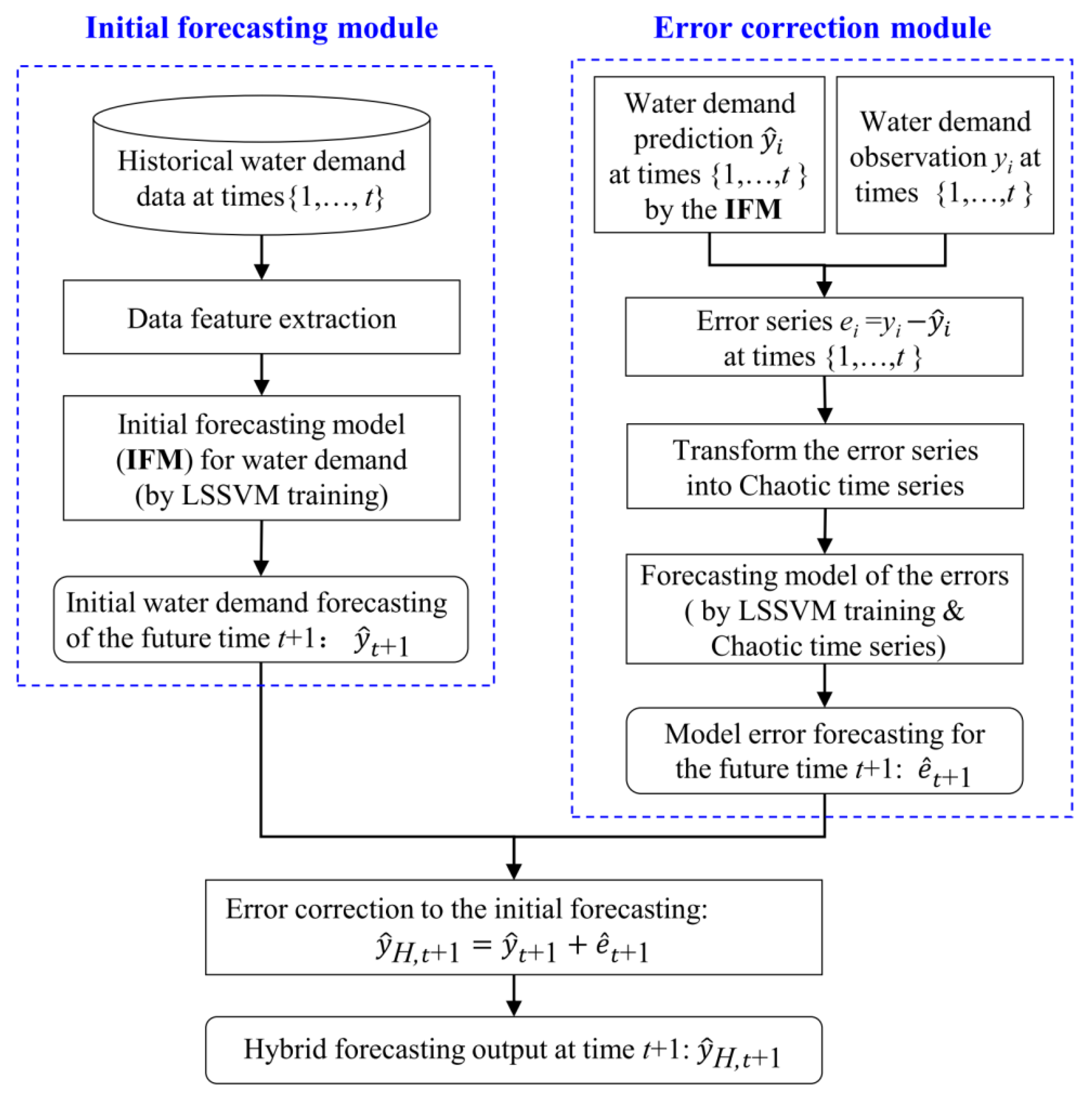
The hybrid forecasting model is mainly constituted of two parts, namely the initial forecasting module and the error correction module. The framework of the hybrid model is shown in Figure 2. The outline of the initial forecasting module is actually similar to the traditional water demand forecasting model. The difference between the hybrid model and the traditional one is the error correction module.
In the initial forecasting module, historical water demand data and other relevant information are firstly collected into a data set with the time step of 15 min. After identification and processing of abnormal data, data features are extracted to provide valuable information to the forecasting model inputs. Furthermore, the nonlinear relationship between the historical water demand data and the demand at the next time step is constructed by LSSVM training, which provides the initial forecasting model F(y) of water demand. Then, the forecasted water demand y ^ t + 1 at the future time (target time) t + 1 is obtained by the initial forecasting model. The errors of the initial forecasting model on the training data at historical time steps (1, …, t) is expressed as:
e i = y i y i ^
where ei is the error of the initial forecasting model at the time step i (i = 1, …, t); yi is the observed water demand at time step i; y i ^ is the output value of the initial forecasting model at time step i. Note that, t + 1 is the first target time step at which the water demand is unknown and needs forecasting.
The error correction module has three steps. Firstly, the error time series (e1, e2, …, ei, …, et) from the initial forecasting model is transformed into a chaotic time series. Secondly, the LSSVM is adopted to establish the relationship between the errors of the initial forecasting at next time step and the chaotic time series at current and previous time steps, which provides the error forecasting model f(e). Thirdly, the forecasted error for the target time t + 1 is obtained and used to correct the initially forecasted demand value as follows:
y ^ H , t + 1 = y ^ t + 1 + e ^ t + 1
where y ^ H , t + 1 is the water demand forecasting by the hybrid model, in other words, the final output of water demand forecasting at the target time t + 1; y ^ t + 1 is the forecasted water demand by the initial forecasting model F(y); and e ^ t + 1 is the forecasted error by the error forecasting model f(e).

2.2. Initial Forecasting Model by LSSVM

SVM has been widely applied in several areas including pattern recognition, regression, nonlinear classification, and function estimation. LSSVM is originated from SVM and first proposed by Suykens and Vandewalle [21], which is believed, takes a computational advantage over standard SVM by converting quadratic optimization problem into linear equations. In the field of water demand forecasting, the LSSVM is used to establish the nonlinear relationship between model inputs and outputs.
Consider a given training set of N samples (Xi; yi)(i = 1, …, N), where Xi denotes the ith input vector in n-dimensional space (Xi = (X1i, …, Xni)∈Rn) and yi is the corresponding desired output value (i.e., the observed value) of the ith sample. The nonlinear function between the inputs and outputs can be given as below [19,26,36]:
y i ^ ( X i ) = ω T φ ( X i ) + b
where y i ^ is the model output corresponding to the sample i, the nonlinear transformation function φ(*) maps the Xi to the m-dimensional feature space, ω is the m-dimensional weight parameter vector, and b is the bias parameter (ωRm, bR).
Equation (3) provides the initial forecasting model of water demand, in other words, the relationship between the model input and output, where the input data is Xi = (Qt, Qt–1, Qt–2, Qt–95, Qt–191, Qt–671) and the output y ^ i is the forecasted water demand Qt+1 at the target time t + 1. Detailed description of model input data selection is presented the Section 3.1.
Considering the complexity of minimizing the model errors between yi and y ^ i , in the LSSVM, the parameters ω and b in equation (3) can be estimated according to the structural risk minimization principle [19,36]:
min   J ( ω , ξ ) = 1 2 ω T ω + 1 2 γ i = 1 N ξ i 2
where γ is the regularization constant determining the tradeoff between the training error and the generalization performance, ξi is a slack variable denotes model error.
The solution of the optimization problem (Equation (4)) can be obtained by Lagrange function [19,36]. Then the LSSVM model for the non-learner function in Equation (3) is finally turned into:
y ^ ( X ) = f ( X ) = i = 1 N α i K ( X i ,   X ) + b
where αi (i = 1, …, N) is the Lagrange multiplier and can be evaluated by γ, K(Xi, X) is the kernel function. The radial basis function (RBF) kernel is one of the most popular kernel functions, and is used in this study as below:
K ( X i , X ) = exp ( | | X i X | | 2 2 σ 2 )
where σ is the width parameter that reflects the radius enclosed by the boundary closure.
It is worth mentioning that, at this point, Equation (3) is transformed into Equation (5) which can be directly established though the training samples (Xi; yi) (i = 1, …, N) and model parameters σ and γ. Therefore, establishing an LSSVM model with RBF kernel involves the selection of RBF kernel width σ and the regularization constant parameter γ. Among the available methods for parameter tuning of LSSVM such as the cross-validation method [19], the grid search method [26], and Bayesian framework-based inferring [13,37], the Bayesian approach with three levels of inference is chosen for parameter tuning of LSSVM in this study.

2.3. Error Forecasting Model Based on Chaotic Time Series

Chaos is a quasi-stochastic irregular motion possibly appearing in deterministic nonlinear dynamic systems [38]. Since various nonlinear systems exhibit chaotic features, chaos theory is widely used in nonlinear system analysis to detect deterministic relationships hidden behind random-looking phenomena, and has been increasingly used in time series analysis [30,31]. According to the delay coordinate embedding technique, the underlying dynamical system can be faithfully reconstructed from stochastic time series under fairly general conditions [39]. Therefore, a one-to-one correspondence can be established between the reconstructed and the true but unknown dynamical systems [40].
Given a scalar time series of model errors e = (e1, e2, …, eN) with time step Δt, and N is the number of elements in the time series, the element ei (i = 1, …, N) is computed by Equation (1). According to the procedure of phase space reconstruction, the scalar time series e is transformed in phase space as follows:
E 1 = ( e 1 ,   e 1 + τ ,   e 1 + 2 τ ,   , e 1 + ( m 1 ) τ ) E 2 = ( e 2 ,   e 2 + τ ,   e 2 + 2 τ ,   , e 2 + ( m 1 ) τ ) E M = ( e M ,   e M + τ ,   e M + 2 τ ,   , e M + ( m 1 ) τ )
where τ is the delay time, it could be several times of Δt; Ei (i = 1, …, M) is a chaotic vector in the phase space, m is the embedding dimension of the phase space, M = N–(m–1)τ is the number of phase point.
Takens [39] has proved that the chaotic attractor of a time series would be revealed in the phase space if the parameters τ and m are properly selected. The dimension parameter m is usually larger than three, to entirely reveal the underlying information of the time series [31]. Among existing methods for determining parameters τ and m, the coupled-cluster (C-C) method [41] is used in this study.
In the case of chaotic systems, the Lyapunov exponent (λ) gives a system the sensitivity to initial conditions and determines the total predictability of the system, and a positive λ indicates the system is chaotic [42]. Therefore, the reconstructed time series (E1, E2, …, EM) is tested for the chaotic signature through the maximum Lyapunov exponent which is evaluated by Wolf’s algorithm [43].
In the phase space of a chaotic system, the dynamic information could be interpreted in the form of m-dimensional mapping as [30]:
E M + 1 = f ( E M )
where EM is the state at current time, EM+1 = (eM+1, eM+1+τ, eM+1+2τ, …, eM+1+(m−1)τ) is the state at future time. Note that, the last element eM+1+(m−1)τ of EM+1 is exactly the next element ek+1 of the error series e which needs to be forecasted. Therefore, the phase point Ei(i = 1, 2, …, M) further evolves into Ei+1, and there is a determinism mapping function between ei+1+(m−1)τ (i.e., the last element of Ei+1) and Ei as follows:
e i + 1 + ( m 1 ) τ = f ( E i ) = f ( e 1 ,   e 1 + τ ,   e 1 + 2 τ ,   , e 1 + ( m 1 ) τ )
According to the properties shown in Equations (8) and (9), the chaotic time series can be utilized for prediction, and then the LSSVM approach described in Section 2.3 can be used to establish the nonlinear functions in Equation (9). The model input data and output data for LSSVM training are shown as follows:
X error = [ E 1 E 2 E M 1 ] ;   Y error = [ e 2 + ( m 1 ) τ e 3 + ( m 1 ) τ e M + ( m 1 ) τ ]
where Xerror is the input data with the dimension of (M–1) × m, Yerror is the output data with the dimension of (M–1) × 1.
Note that, due to M = N–(m–1)τ, the last element of Yerror is actually eN, in other words, the last element of the error time series e. After the nonlinear function of Equation (9) is established by LSSVM, one can predict the future element of e at next time step through eN+1 = f(EM).

2.4. Performance Indicators of Forecasting Models

In terms of accuracy evaluation of water demand forecasting models, variety of measures are available to characterize the performance of the models [1,7,9]. This study adopts four widely used indicators as evaluation criteria, including the mean absolute error (MAE), the mean absolute percentage error (MAPE), the root means square error (RMSE), and the coefficient of determination (R2). The equations of these aforementioned indicators are shown as follows:
MAE = 1 N f i = 1 N f | y i y ^ i |
MAPE = 1 N f i = 1 N f | y i y ^ i | y i × 100 %
RMSE = 1 N f i = 1 N f ( y i y ^ i ) 2
R 2 = 1 i = 1 N f ( y i y ^ i ) 2 i = 1 N f ( y i y ¯ ) 2
where yi and y ^ i are the observed value and the predicted value of water demand at time i, respectively; y ¯ and y ^ ¯ are the corresponding mean values; Nf is the number of forecasted time steps, which is equal to 96 for the water demand forecasting problem with a one day horizon and a frequency of 15 min.

3. Case Study

3.1. Data Feature Extraction and Model Inputs

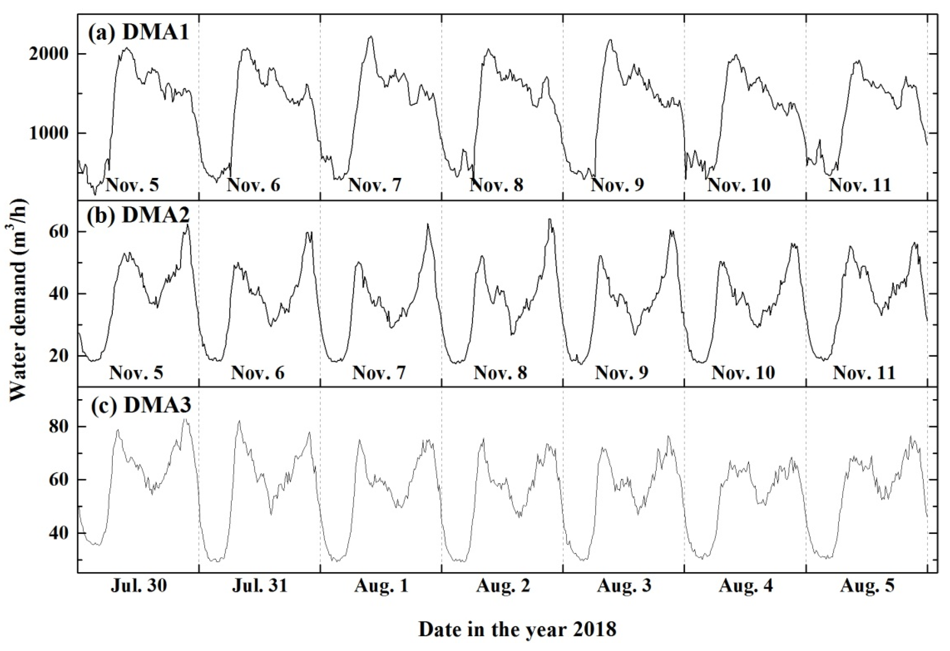
The historical water demand data from three actual DMAs (namely, DMA1, DMA2, and DMA3) in Beijing, China, were collected and used to train and test the forecasting model. On the inlet of the DMA, the water demand data were metered with the unit of m3 and recorded every 15 min; then the data were transferred to the database of the Beijing Water Works in real time. The water consumption pattern and the composition of customers in DMA1 is very different from that in DMA2 and DMA3; DMA1 includes more than 10,000 residential customers, 168 business customers, and 68 industrial customers. The number of water customers in DMA2 and DMA3 are 1822 and 1936, respectively; water customers in DMA2 and DMA3 are mostly residential and there are also some business customers. The statistics of the three DMAs’ water consumption data are show in Table 1. The three DMAs’ water consumptions at different times in one week are shown in Figure 3. From the weekly curves of water demands in Figure 3, one can see the different demand patterns of the three DMAs, for example, there is no obvious peak hour in the evening for DMA1, and there are no obvious morning peak hours on weekends for DMA3.
In total, 8 weeks’ data were collected from the water demand record in 2018 for training and testing the forecasting model. The data set contains 5376 observations for each DMA. Seven weeks’ data were used as training data, while the last week’s data were used for model testing. When using the hybrid framework to predict the water demand at 96 time steps on the next day, the water demand data of the current day and previous days were used for model training, for example, the historical water demand data of the previous 49 days were used for model training to predict the demand on the 50th day, and the water demand data of the previous 50 days were used for model training to predict the demand on day 51, and so on.
When selecting the input data for the forecasting model from the historical water demand data, Guo et al. [9] categorized the historical data into three fragments, namely, recent time, near time, and distant time, and selected five time-steps in each time fragment as the input data. Herrera et al. [1] selected the historical water demand data at three time-steps including the current time, the previous time, and the target time in the previous week as the input data. Ordan and Reis [7] selected six time-steps including four continuous time-steps before the target time, the target time on the previous day, and previous week. According to these literatures, the historical water demand at the current time, the previous time, the target time on the previous day, and the previous week are usually adopted as the model input data in the short-term water demand forecasting. In this study, to better model the characteristics of the water demand time series, a correlation analysis [7] is performed based on the data of three DMAs to find the data that is highly related to the water demand data at the target time from the historical water demand data. Furthermore, various combinations of the related data are tested as the input for the forecasting model, and the following combination is identified as having the best performance, in other words, three continuous time-steps before the target time (Qt, Qt–1, Qt–2), the target time on the previous one day and two days (Qt–95 and Qt–191), and the target time on the previous week (Qt–671). Therefore, the historical data set (Qt, Qt–1, Qt–2, Qt–95, Qt–191, Qt–671) is adopted as the input data for the initial forecasting model in this study.

3.2. Model Setup

In addition to the hybrid forecasting model proposed in this study, two other forecasting models are established to make comparisons with and to validate the performance of the proposed hybrid forecasting approach. As summarized in Table 2, the hybrid model H_LSSVM_Chaos is the one established by the hybrid framework of this study (see Figure 2), and the other two are a single forecasting (S_LSSVM) and a hybrid forecasting model (H_LSSSVM_FS), respectively. The single forecasting model S_LSSVM uses the traditional prediction procedure without error correction module, in other words, only the initial forecasting module is used. The hybrid forecasting model (H_LSSVM_Chaos and H_LSSSVM_FS) adopts both the initial forecasting module and the error correction module. The model inputs of the initial forecasting module are the feature data extracted from the historical water demand data, while the model inputs of the error correction module are the error series of the initial forecasting model. The error series can be evaluated according to Equation (1) and the flowchart in Figure 2. In the hybrid forecasting model, the initial forecasting module is the same one applied in the single forecasting model.
The hybrid model H_LSSSVM_FS uses the Fourier series as the forecasting model of the error time series in the error correction module, which is similar to the approach used by Brentan et al. [29] and Ordan and Reis [7]. Model inputs of the hybrid models’ error correction modules are based on the errors of the initial forecasting by the S_LSSVM model.
For the error correction module in the H_LSSVM_FS model, the error time series of the previous seven days (i.e., 672 values) is used to compute the coefficients of the Fourier series; the number of harmonics of FS is set to 336. The LS-SVMlab Toolbox developed by Brabanter et al. [44] is used to train the forecasting models by LSSVM, and the three-Level Bayesian inferring method is adopted for parameter tuning of the LSSVM. Table 3 displays the model parameters for the application of LSSVM and chaos methods. Parameters γ and δ2 in Table 3 were obtained by Bayesian method for the LSSVM model training. In addition, m and τ are the essential parameters for chaotic time series construction.

3.3. Application Results

3.3.1. Overall Performance

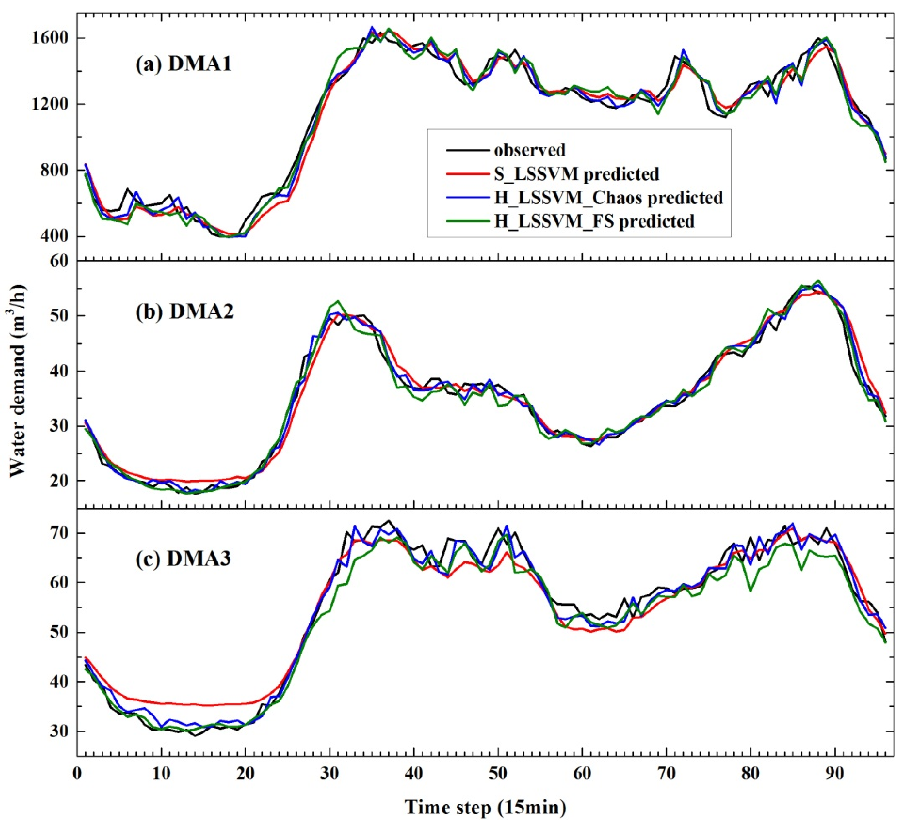
Figure 4 compares the observed water demand with the forecasted water demand using the S_LSSVM, H_LSSVM_Chaos, and H_LSSVM_FS models at 15 min steps for one day ahead. It can be seen that the predicted water demand by the three models is consistent with the trend of the observations, and the hybrid models perform better than the single forecasting models (S_LSSVM) during the periods of water demand fluctuations. As quantified below by the model performance indicators, the H_LSSVM_Chaos models provide the closest estimates to the corresponding observed water demand during most of the peak periods.
Table 4 gives the overall performance of the different forecasting models for the three DMAs in Beijing. It can be seen that the H_LSSVM_Chaos provides a higher accuracy than the other two models according to the performance indicators R2, MAE, MAPE, and RMSE. The single forecasting model S_LSSVM is the least accurate.
Among the three DMAs, the prediction accuracy to DMA1 is slightly worse than to DMA2 and DMA3, for example, the MAPEs of (DMA1, DMA2, DMA3) of the H_LSSVM_Chaos models and the H_LSSVM_FS models are (4.84%, 3.15%, 3.47%) and (5.44%, 3.33%, 3.72%), respectively. The reason is that the composition of the water customers in DMA1 is relatively complex, not only including residential users, but also a large number of commercial and industrial users. The statistical parameter COV of DMA1′s water demand data is 0.39, which is the largest one among the three DMAs. Larger COV indicates a high level of water demand floating and makes the demand pattern more difficult to capture. As a result, even using the error correction module, the hybrid model H_LSSVM_Chaos only reduced the MAPE of DMA1 from 5.64% to 4.84%, which is less than the reductions for the other DMAs. Moreover, because the water consumptions in DMA2 are mostly residential demands which thus lead to a simple water demand pattern, the prediction results for DMA2 give the highest accuracy. Therefore, as for the error correction module performance on short-term water demand forecasting, the DMAs with simple customer composition have better prediction accuracy when using error correction module.

3.3.2. Comparisons Between the Hybrid Forecasting Models

Figure 5 shows the error forecasting by the error correction module in the hybrid models. Compared to the water demand data in Figure 4, the errors of initial forecasting in Figure 5 have a large number of fluctuations, in other words, the value of errors has a greater frequency of change. In addition, the complex and disorderly change in the peak values of the error data are also shown in Figure 5; there is no obvious rule on the occurrence time of the peak value, such as peaks at the time steps (7, 45, 71, 75) in Figure 5a. The results in Figure 5 can be summarized as follows:
  • The error forecasting models based on the chaos method and the FS method can both obtain more reasonable prediction results in some periods where the error data changes mildly, such as time steps 5 to 23 and 60 to 72 in DMA2, and 10 to 24 in DMA3.
  • The prediction accuracy of the two methods is relatively low in the periods where the error data change frequently, such as time steps 33 to 55 in DMA1, 24 to 34 in DMA2, and 35 to 53 in DMA3. It should be noted that even in these hardly predictable time steps, however, the predictions from the chaos method is closer to the errors of the initial prediction than the FS model, e.g., for the error predictions at time steps 30 to 55 in the three DMAs, the MAEs obtained by chaos method and FS model are (47.54, 1.17, 2.40) and (64.53, 1.84, 3.15), respectively.
  • At some time steps, the error predictions from the FS method are larger than the errors of initial prediction, which leads to misleading corrections to the initial forecasting, such as the time steps 32, 33, and 62 to 64 in DMA1; time steps 32, 46, 55 and 50 in DMA2; time steps 30 to 35, 80 and 86 in DMA3. While this kind of misleading correction is not much in the chaos method.
In general, the chaos method performs better than the FS method in predicting such a complex fluctuated error time series, and the practice also proves that the errors predicted by the chaotic method are closer to the initial errors in the three DMAs.
The statistics of absolute percentage errors (APE) between the single forecasting model S_LSSVM and the hybrid models are provided in Figure 6. From the mean, median, maximum, and minimum values of APEs of the predictions for the three DMAs in Beijing, the H_LSSVM_Chaos models perform better than that of the S_LSSVM models. Therefore, the hybrid framework using the LSSVM and chaotic time series gives more accurate predictions. The hybrid models using LSSVM and Fourier series did not always perform as well as the H_LSSVM_Chaos. The MAPEs of the H_LSSVM_FS model for DMA1 is 5.44%, which is better than that of the single forecasting model S_LSSVM 5.68%. Whereas, other statistics of the H_LSSVM_FS model in DMA1, such as the 75-percentile value and the maximum value of the APE, are similar or even worse than that of the S_LSSVM. The reason is that the H_LSSVM_FS model performs a misleading correction for the severely fluctuated time steps, as shown in Figure 5a. For DMA2, although the mean and median APEs of the H_LSSVM_FS models are similar to that of the H_LSSVM_Chaos models, the overestimates of the errors during the time steps 38 to 58 in Figure 5b by the FS method are still notable. Therefore, more attention should be paid when using the error correction module in short-term water demand forecasting.

3.4. Discussion

In the initial forecasting module and error correction module of the hybrid forecasting framework, the forecasting models are established by LSSVM. The successful implementation of the LSSVM model depends on the precision of model parameters (i.e., γ and δ2). In this study, the three-level Bayesian evidence inferring method is adopted to infer LSSVM model parameters. To investigate the influence of model parameters on the performance of LSSVM models, the application of the S_LSSVM model on DMA2 is taken as an example. With the same model input data, Table 5 shows the model performances to different model parameters which are obtained by the 1-level Bayesian inferring, 3-level Bayesian inferring, and the grid search algorithm. These parameters are computed by the LS-SVMlab Toolbox [45]. As Table 5 shows, after 3-level inferring, the Bayesian evidence method catches reasonable model parameters with moderate computation burden. The grid search algorithm provides the best performance, but it takes the longest computation time. As shown in Table 4, the hybrid model H_LSSVM_Chaos model using 3-level Bayesian inferred parameters performs even better than the grid search algorithm built S_LSSVM model. The computation time of the H_LSSVM_Chaos model is about 1 time (including initial forecasting and error correction) longer than the 3-level Bayesian built S_LSSVM model, which is much shorter than that of the grid search algorithm built S_LSSVM model (Table 5). Therefore, the hybrid framework using 3-level Bayesian built LSSVM for initial forecasting and error time series forecasting is suitable for the short-term water demand forecasting.
The hybrid model (H_LSSVM_Chaos) is also compared to the traditional ARIMA model, and Table 6 shows the results on the three DMAs. The development of the ARIMA models follows the procedure described by Adamowski [45]. The parameters of the ARIMA are trained and tested based on different combinations, the number of autoregressive parameters (p), the number of difference (d) and the number of moving average parameters (q) are set as (3, 1, 1). Note that, the same set of historical water demand data are used to build the H_LSSVM_Chaos and ARIMA forecasting models; the historical data before the forecasting day are used to establish the forecasting models.
As shown in Table 6, the H_LSSVM_Chaos model perform better than the ARIMA model on DMA1 and DMA2, for example, the MAPEs (DMA1, DMA2) of the H_LSSVM_Chaos model and the ARIMA model are (4.84%, 3.15%) and (5.53%, 3.83%), respectively. Whereas, the application results of DMA3 show some variations: (i) on the forecasting day August 11, the H_LSSVM_Chaos has a similar result to the ARIMA, for example, the R2 and MAPEs of the two models are (0.9701, 0.9687) and (3.47%, 3.44%), respectively; (ii) on the forecasting days from August 8 to 10, the H_LSSVM_Chaos perform better than the ARIMA, for example, the three days’ MAPEs of the H_LSSVM_Chaos and the ARIMA are (3.48%, 2.81%, 2.71%) and (4.03%, 3.10%, 3.35%), respectively. The reason for the variations is that August 11 is Saturday while August 8 to 10 are weekdays. As shown in Figure 3c and Figure 4c, for DMA3, the water consumption curve on Saturday is different and more complex than that of weekdays. The distinctive water consumption curve on Saturday results in fewer training samples for establishing the forecasting model, which affects the forecasting accuracy for Saturday. However, the overall performance of the H_LSSVM_Chaos model is still better than the ARIMA model, despite the variations in the forecasting accuracy on Saturday. These comparisons verified the validity of the H_LSSVM_Chaos model.
Generally, one single model could not identify the underlying patterns for every case, and the hybrid framework including different models is able to capture different aspects of the available information for prediction [5,46]. The LSSVM method in the initial prediction module captures nonlinear relationships between the discontinuous feature data (Qt, Qt–1, Qt–2, Qt–95, Qt–191, Qt–671) of the historical water demand data set and the water demand Qt+1 on the forecasting day; the chaotic time series method in the error correction module captures the continuous and periodic changes from the errors of the initial forecasting module.

4. Conclusions

Short-term water demand forecasting with the horizon ranges from sub-hourly to daily plays an important role in the field of optimal operation of pump stations and online hydraulic simulation of water distribution systems. To obtain more accurate predictions, this study proposes a hybrid framework with the error correction module which uses the chaotic time series, and investigates the performance of the framework in the short-term water demand forecasting with one day ahead and a 15-min time step. The hybrid framework is developed by integrating two modules, namely, the initial forecasting module and the error correction module. The initial forecasting model is established by the least squares support vector machines (LSSVM). In the error correction module the errors forecasting model is established by LSSVM using chaotic time series of error data from initial forecasting.
The hybrid model is implemented in the water demand forecasting of three actual district metering areas (DMAs) in Beijing, China, and the application results of the hybrid model are comparable to that of other two models including the forecasting model without error correction and the hybrid model using Fourier series for error correction. From the case study results, the following conclusions could be drawn:
  • In most instances, the hybrid models perform better than the forecasting model without error correction. The error correction module performs better in the short-term water demand forecasting than the DMAs whose composition of customers is simple. A simple composition of customers indicates a simple water consumption pattern and less peak fluctuations in the water consumption curves.
  • Due to the capability of detecting the underlying instability characteristics of time series, the error correction module using chaotic time series performs better than the Fourier series in predicting a complex disordered time series of errors.
  • For the periods of frequent and disordered peak fluctuations in the error time series, the performance of the error correction module is not good, and the error forecasting model based on Fourier series may lead to unreasonable forecasts by misleading the corrections to the initial forecasting. As a result, more attention should be paid to the features of the error time series when using the error correction module.
In the presented study, the hybrid forecasting framework is tested by three actual DMAs in Beijing with different characteristics. Further work on other DMAs are needed to test and verify the robustness of the hybrid forecasting framework, and much more effort is needed to test the performance of chaotic methods in mining the characteristics of the disordered peak fluctuated data. This study only tested the proposed model for the 24 h forecast horizon, whereas, the hybrid forecasting framework is not limited to the forecast horizon of one day, there is a potential to implement the model to a much longer forecast horizon and frequency, such as one week ahead with a time step of 6 h. Then the feature data for model training obtained from the historical data set should be adjusted accordingly.

Author Contributions

Conceptualization, S.W. and B.H.; methodology, H.H. and B.H.; validation, S.W., H.H., B.H., and K.D.; formal analysis, H.H., B.H., and K.D.; investigation, H.H., B.H., and K.D.; resources, S.W., H.H., B.H., and K.D.; writing—original draft preparation, H.H. and B.H.; writing—review and editing, S.W. and K.D.; visualization, B.H. and K.D.; supervision, S.W.; project administration, S.W. and B.H.; funding acquisition, S.W. All authors have read and agreed to the published version of the manuscript.

Funding

This research was funded by the Major Science and Technology Program for Water Pollution Control and Treatment, grant number 2017ZX07108-002.

Acknowledgments

The authors would like to thank the editors and reviewers for bringing the paper to a scientific standard for inclusion in the journal.

Conflicts of Interest

The authors declare no conflict of interest.

References

  1. Herrera, M.; Torgo, L.; Izquierdo, J.; Pérez-García, R. Predictive models for forecasting hourly urban water demand. J. Hydrol. 2010, 387, 141–150. [Google Scholar] [CrossRef]
  2. Anele, A.; Hamam, Y.; Abu-Mahfouz, A.; Todini, E. Overview, comparative assessment and recommendations of forecasting models for short-term water demand prediction. Water 2017, 9, 887–898. [Google Scholar] [CrossRef] [Green Version]
  3. Chen, J.; Boccelli, D.L. Demand forecasting for water distribution systems. Procedia Eng. 2014, 70, 339–342. [Google Scholar] [CrossRef] [Green Version]
  4. Qin, T.; Boccelli, D.L. Estimating distribution system water demands using Markov chain Monte Carlo. J. Water Resour. Plan. Manag. 2019, 145, 04019023. [Google Scholar] [CrossRef]
  5. Donkor, E.A.; Mazzuchi, T.A.; Soyer, R.; Alan Roberson, J. Urban water demand forecasting: Review of methods and models. J. Water Resour. Plan. Manag. 2014, 140, 146–159. [Google Scholar] [CrossRef]
  6. Chen, J.; Boccelli, D.L. Forecasting hourly water demands with seasonal autoregressive models for real-time application. Water Resour. Res. 2018, 54, 879–894. [Google Scholar] [CrossRef]
  7. Odan, F.K.; Reis, L.F.R. Hybrid water demand forecasting model associating artificial neural network with Fourier series. J. Water Resour. Plan. Manag. 2012, 138, 245–256. [Google Scholar] [CrossRef] [Green Version]
  8. Pacchin, E.; Gagliardi, F.; Alvisi, S.; Franchini, M. A comparison of short-term water demand forecasting models. Water Resour. Manag. 2019, 33, 1481–1497. [Google Scholar] [CrossRef]
  9. Guo, G.; Liu, S.; Wu, Y.; Li, J.; Zhou, R.; Zhu, X. Short-term water demand forecast based on deep learning method. J. Water Resour. Plan. Manag. 2018, 144, 04018076. [Google Scholar] [CrossRef]
  10. Crommelynck, V.; Duquesne, C.; Mercier, M. Daily and Hourly Water Consumption Forecasting Tools Using Neural Networks. In Proceeding of the AWWA’s Annual Computer Specialty Conference, Nashville, TN, USA, 12–15 April 1999; pp. 665–676. [Google Scholar]
  11. Jain, A.; Ormsbee, L. Short-term water demand forecast modeling techniques—Conventional Methods Versus AI. Am. Water Work. Assoc. 2002, 94, 64–72. [Google Scholar] [CrossRef]
  12. Bougadis, J.; Adamowski, K.; Diduch, R. Short-term municipal water demand forecasting. Hydrol. Process. 2005, 19, 137–148. [Google Scholar] [CrossRef]
  13. Chen, L.; Zhang, T.Q. Hourly water demand forecast model based on Bayesian least squares support vector machine. J. Tianjin Univ. 2006, 39, 1037–1042. [Google Scholar]
  14. Chen, L.; Zhang, T.Q. Hourly water demand forecast model based on least squares support vector machine. J. Harbin Inst. Technol. 2006, 38, 1528–1530. [Google Scholar]
  15. Khan, M.S.; Coulibaly, P. Application of support vector machine in lake water level prediction. J. Hydrol. Eng. 2006, 11, 199–205. [Google Scholar] [CrossRef]
  16. Braun, M.; Bernard, T.; Piller, O.; Sedehizade, F. 24-Hours demand forecasting based on SARIMA and support vector machines. Procedia Eng. 2014, 89, 926–933. [Google Scholar] [CrossRef]
  17. Dahl, C.M.; Hylleberg, S. Flexible regression models and relative forecast performance. Int. J. Forecast. 2004, 20, 201–217. [Google Scholar] [CrossRef]
  18. Chen, G.; Long, T.; Xiong, J.; Bai, Y. Multiple random forests modelling for urban water consumption forecasting. Water Resour. Manag. 2017, 31, 4715–4729. [Google Scholar] [CrossRef]
  19. Tripathi, S.; Srinivas, V.V.; Nanjundiah, R.S. Downscaling of precipitation for climate change scenarios: A support vector machine approach. J. Hydrol. 2006, 330, 621–640. [Google Scholar] [CrossRef]
  20. Ghalehkhondabi, I.; Ardjmand, E.; Young, W.A.; Weckman, G.R. Water demand forecasting: Review of soft computing methods. Env. Monit Assess. 2017, 189, 313. [Google Scholar] [CrossRef]
  21. Suykens, J.A.K.; Vandewalle, J. Least squares support vector machine classifiers. Neural Process. Lett. 1999, 9, 293–300. [Google Scholar] [CrossRef]
  22. Suykens, J.A.K.; De Brabanter, J.; Lukas, L.; Vandewalle, J. Weighted least squares support vector machines robustness and sparse approximation. Neurocomputing 2002, 48, 85–105. [Google Scholar] [CrossRef]
  23. Vijai, P.; Bagavathi Sivakumar, P. Performance comparison of techniques for water demand forecasting. Procedia Comput. Sci. 2018, 143, 258–266. [Google Scholar] [CrossRef]
  24. Samsudin, R.; Saad, P.; Shabri, A. River flow time series using least squares support vector machines. Hydrol. Earth Syst. Sci. 2011, 15, 1835–1852. [Google Scholar] [CrossRef] [Green Version]
  25. Kisi, O. Modeling discharge-suspended sediment relationship using least square support vector machine. J. Hydrol. 2012, 456–457, 110–120. [Google Scholar] [CrossRef]
  26. Aydogdu, M.; Firat, M. Estimation of failure rate in water distribution network using fuzzy clustering and LS-SVM methods. Water Resour. Manag. 2014, 29, 1575–1590. [Google Scholar] [CrossRef]
  27. Cherkassky, V.; Ma, Y. Practical selection of SVM parameters and noise estimation for SVM regression. Neural Netw. 2004, 17, 113–126. [Google Scholar] [CrossRef] [Green Version]
  28. Zhang, G.P. Time series forecasting using a hybrid ARIMA and neural network model. Neurocomputing 2003, 50, 159–175. [Google Scholar] [CrossRef]
  29. Brentan, B.M.; Luvizottom, E.; Herrera, M.; Izquierdo, J.; Pérez-García, R. Hybrid regression model for near real-time urban water demand forecasting. J. Comput. Appl. Math. 2017, 309, 532–541. [Google Scholar] [CrossRef]
  30. Dhanya, C.T.; Nagesh Kumar, D. Multivariate nonlinear ensemble prediction of daily chaotic rainfall with climate inputs. J. Hydrol. 2011, 403, 292–306. [Google Scholar] [CrossRef]
  31. Liu, X.; Fang, X.; Qin, Z.; Ye, C.; Xie, M. A Short-term forecasting algorithm for network traffic based on Chaos theory and SVM. J. Netw. Syst. Manag. 2010, 19, 427–447. [Google Scholar] [CrossRef]
  32. Yang, H.Y.; Ye, H.; Wang, G.; Khan, J.; Hu, T. Fuzzy neural very-short-term load forecasting based on chaotic dynamics reconstruction. Chaos Solitons Fractals 2006, 29, 462–469. [Google Scholar] [CrossRef]
  33. Bakker, M.; Vreeburg, J.H.G.; van Schagen, K.M.; Rietveld, L.C. A fully adaptive forecasting model for short-term drinking water demand. Environ. Model. Softw. 2013, 48, 141–151. [Google Scholar] [CrossRef]
  34. Cutore, P.; Campisano, A.; Kapelan, Z.; Modica, C.; Savic, D. Probabilistic prediction of urban water consumption using the SCEM-UA algorithm. Urban. Water J. 2008, 5, 125–132. [Google Scholar] [CrossRef]
  35. Al-Zahrani, M.A.; Abo-Monasar, A. Urban residential water demand prediction based on artificial neural networks and time series models. Water Resour. Manag. 2015, 29, 3651–3662. [Google Scholar] [CrossRef]
  36. Van Gestel, T.; Suykens, J.A.; Baesens, B.; Viaene, S.; Vanthienen, J.; Dedene, G. Benchmarking least squares support vector machine classifiers. Mach. Learn. 2004, 54, 5–32. [Google Scholar] [CrossRef]
  37. Van Gestel, T.; Suykens, J.A.; Baestaens, D.E.; Lambrechts, A.; Lanckriet, G.; Vandaele, B. Financial time series prediction using least squares support vector machines within the evidence framework. IEEE Trans. Neural Netw. 2001, 4, 809–821. [Google Scholar] [CrossRef] [Green Version]
  38. Li, D.; Han, M.; Wang, J. Chaotic time series prediction based on a novel robust echo state network. Trans. Neural Netw. Learn. Syst. 2012, 23, 787–799. [Google Scholar] [CrossRef]
  39. Takens, F. Detecting strange attractors in turbulence. In Lecture Notes in Mathematics; Rand, D.A., Young, L.S., Eds.; Springer: Berlin, Germany, 1981; Volume 898, pp. 366–381. [Google Scholar] [CrossRef]
  40. Lai, Y.C.; Ye, N. Recent developments in chaotic time series analysis. World Sci. Publ. Co. 2003, 13, 1383–1422. [Google Scholar] [CrossRef]
  41. Kim, H.S.; Eykholt, R.; Salas, J.D. Nonlinear dynamics, delay times, and embedding windows. Phys. D Nonlinear Phenom. 1999, 127, 48–60. [Google Scholar] [CrossRef]
  42. Dhanya, C.T.; Nagesh Kumar, D. Nonlinear ensemble prediction of chaotic daily rainfall. Adv. Water Resour. 2010, 33, 327–347. [Google Scholar] [CrossRef]
  43. Wolf, A.; Swift, J.B.; Swinney, H.L.; Vastano, J.A. Determining Lyapunov exponents from a time series. Phys. D Nonlinear Phenom. 1985, 16, 285–317. [Google Scholar] [CrossRef] [Green Version]
  44. De Brabanter, K.; Karsmakers, P.; Ojeda, F. LS-SVMlab Toolbox User’s Guide Version 1.8; Katholieke Universiteit Leuven: Leuven, Belgium, 2011; p. 115. [Google Scholar]
  45. Adamowski, J.F. Development of a short-term river flood forecasting method for snowmelt driven floods based on wavelet and cross-wavelet analysis. J. Hydrol. 2008, 353, 247–266. [Google Scholar] [CrossRef]
  46. Wang, X.; Sun, Y.; Song, L.; Mei, C. An eco-environmental water demand based model for optimising water resources using hybrid genetic simulated annealing algorithm. Part II: Model application and results. J. Environ. Manag. 2009, 19, 2612–2619. [Google Scholar] [CrossRef] [PubMed]
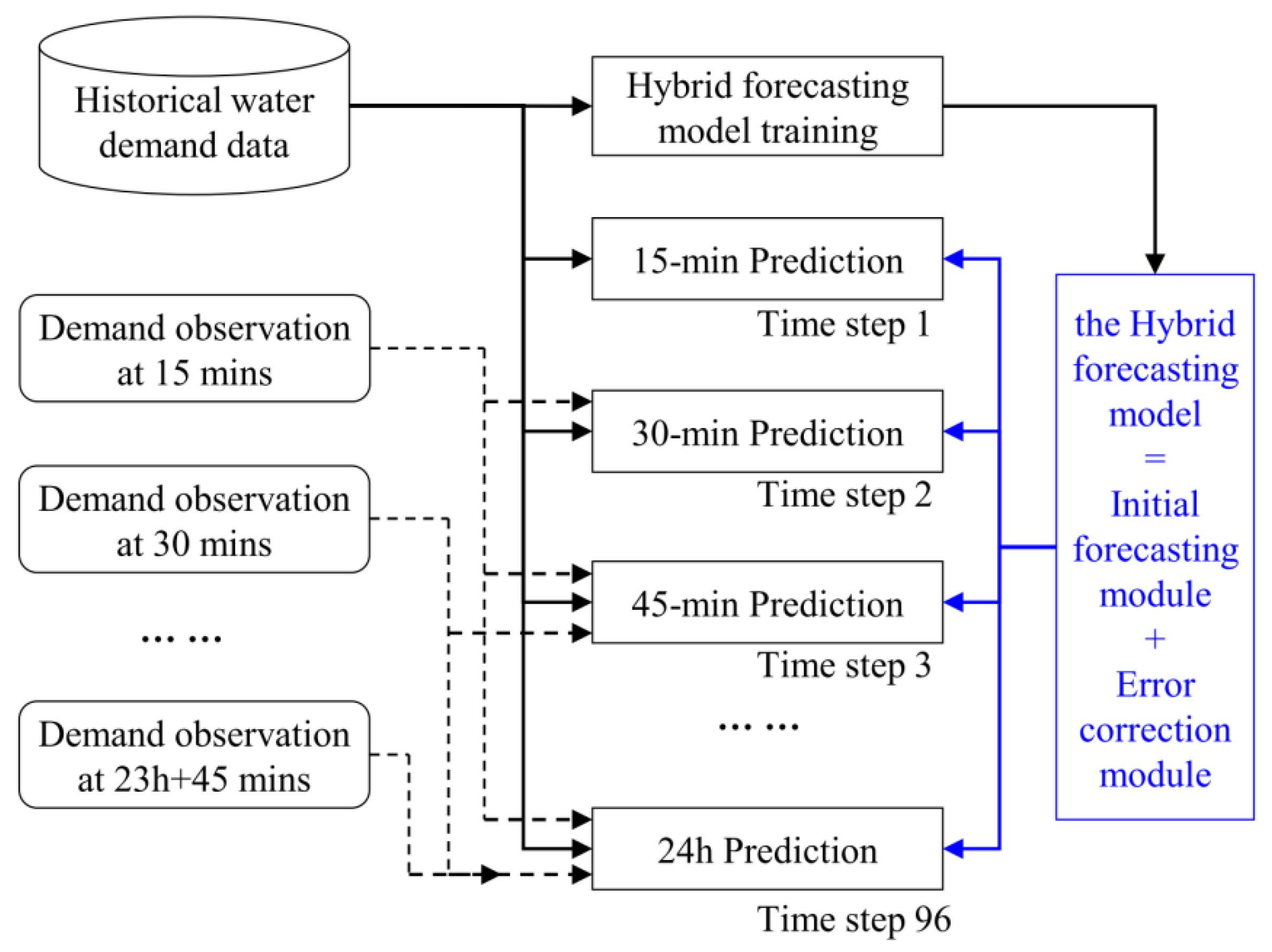
Figure 1. Water demand data processing procedure.
Water 12 01683 g001
Figure 2. Hybrid framework for water demand forecasting.
Water 12 01683 g002
Figure 3. One-week water consumption curves of the case study DMAs. (a) DMA1; (b) DMA2, and (c) DMA3.
Water 12 01683 g003
Figure 4. Water demand forecasting for one day ahead with the time step of 15 min. (a) Water demand of DMA1 on 26 December; (b) water demand of DMA2 on 26 December; and (c) water demand of DMA3 on 11 August.
Water 12 01683 g004
Figure 5. Comparison between the errors of the initial forecasting and the predicted errors. (a) DMA1 on 26 December; (b) DMA2 on 26 December; and (c) DMA3 on 11 August.
Water 12 01683 g005
Figure 6. Statistics of the absolute relative errors for different forecasting models.
Water 12 01683 g006
Table 1. Characteristics of water demand data in 2018 for the three case study district metering areas (DMAs).
DMAsDate of DataMinimum (m³/h)Maximum (m³/h)Mean (m³/h)Standard Deviation (m³/h)Coefficient of Variation
DMA11 November–26 December120.002224.001192.03467.810.39
DMA21 November–26 December16.8867.0435.8519.970.30
DMA317 June–11 August28.4895.1263.4515.140.24
Table 2. Characteristics of forecasting models.
ModelsForecasting CategoryModel Inputs
S_LSSVMSingle forecastingFeature values of historical water demand data
H_LSSVM_ChaosHybrid forecastingChaotic time series of the errors of the initial forecasting
H_LSSVM_FSHybrid forecastingScalar time series of the errors of the initial forecasting
Table 3. Model parameters for the application of LSSVM and chaos methods.
ModelsDMA IDγδ2mτ
S_LSSVM10.14315.7407--
20.037812.5104--
30.045713.4042--
H_LSSVM_Chaos10.58275.768049
22.78724.558648
33.12696.1330311
Table 4. Performance indicators of forecasting models on testing data.
ModelsDMA IDR2MAE (m3/h)MAPE (%)RMSE (m3/h)
S_LSSVM10.965454.435.6468.61
20.97221.314.061.76
30.94472.705.843.31
H_LSSVM_Chaos10.971147.924.8462.66
20.98171.083.151.43
30.97011.863.472.44
H_LSSVM_FS10.962656.355.4471.30
20.97821.183.331.56
30.95332.203.723.05
Table 5. Performances of the S_LSSVM model with different parameters with application to DMA2.
MethodsModel ParametersModel Performance IndicatorsComputation Time (s)
γδ2R2MAE (m3/h)MAPE (%)RMSE (m3/h)
1-level Bayesian inferring 0.018313.67630.96321.564.982.03179
3-level Bayesian inferring 0.037812.51040.97221.314.061.761253
Grid search0.10970.75150.98091.133.381.463685
Table 6. Performance comparison between the auto regressive integrated moving average (ARIMA) and the hybrid forecasting models.
DMA IDForecasting DateForecasting ModelsR2MAE (m3/h)MAPE (%)RMSE (m3/h)
126 DecemberARIMA0.9656 55.43 5.5368.34
H_LSSVM_Chaos0.971147.924.8462.66
226 DecemberARIMA0.9723 1.31 3.831.76
H_LSSVM_Chaos0.98171.083.151.43
311 AugustARIMA0.9687 1.92 3.442.50
H_LSSVM_Chaos0.97011.863.472.44
8–10 August (mean values)ARIMA0.96871.903.492.44
H_LSSVM_Chaos0.97721.643.002.08