Characterizing Hydrological Drought and Water Scarcity Changes in the Future: A Case Study in the Jinghe River Basin of China

Abstract

The assessment of future climate changes on drought and water scarcity is extremely important for water resources management. A modeling system is developed to study the potential status of hydrological drought and water scarcity in the future, and this modeling system is applied to the Jinghe River Basin (JRB) of China. Driven by high-resolution climate projections from the Regional Climate Modeling System (RegCM), the Variable Infiltration Capacity model is employed to produce future streamflow projections (2020–2099) under two Representative Concentration Pathway (RCP) scenarios. The copula-based method is applied to identify the correlation between drought variables (i.e., duration and severity), and to further quantify their joint risks. Based on a variety of hypothetical water use scenarios in the future, the water scarcity conditions including extreme cases are estimated through the Water Exploitation Index Plus (WEI+) indicator. The results indicate that the joint risks of drought variables at different return periods would decrease. In detail, the severity of future drought events would become less serious under different RCP scenarios when compared with that in the historical period. However, considering the increase in water consumption in the future, the water scarcity in JRB may not be alleviated in the future, and thus drought assessment alone may underestimate the severity of future water shortage. The results obtained from the modeling system can help policy makers to develop reasonable future water-saving planning schemes, as well as drought mitigation measures.

1. Introduction

Drought and water scarcity (WS) are inevitable research topics for water resource management in water-stressed areas [1,2,3]. Drought is a natural disaster that affects a large number of people and causes huge economic losses in the world [4,5]. WS is usually caused by the combined effects of natural factors and excessive water uses of human beings, and has already become a vital obstacle for socio-economic development in many parts of the world [6]. In the context of global climate change, many traditional arid regions may experience more severe drought events in the future, which have even been observed in the past few years [7,8,9]. Moreover, due to the increase in population and the improvement of living standards, water usage is significantly growing, which will result in massive WS in numerous regions in the future [2,10,11]. Consequently, it is desired to explore the severity of drought and further reveal the associated WS under climate change in order to manage water resources reasonably and meet the needs of sustainable development [6,11].

Drought can be classified from meteorology, agriculture, hydrology and socioeconomic aspects [12]. Among the four types of drought, hydrological drought (HD) can characterize the reduction of water resources in the terrestrial phase of hydrological cycles such as rivers, lakes and reservoirs [13]. 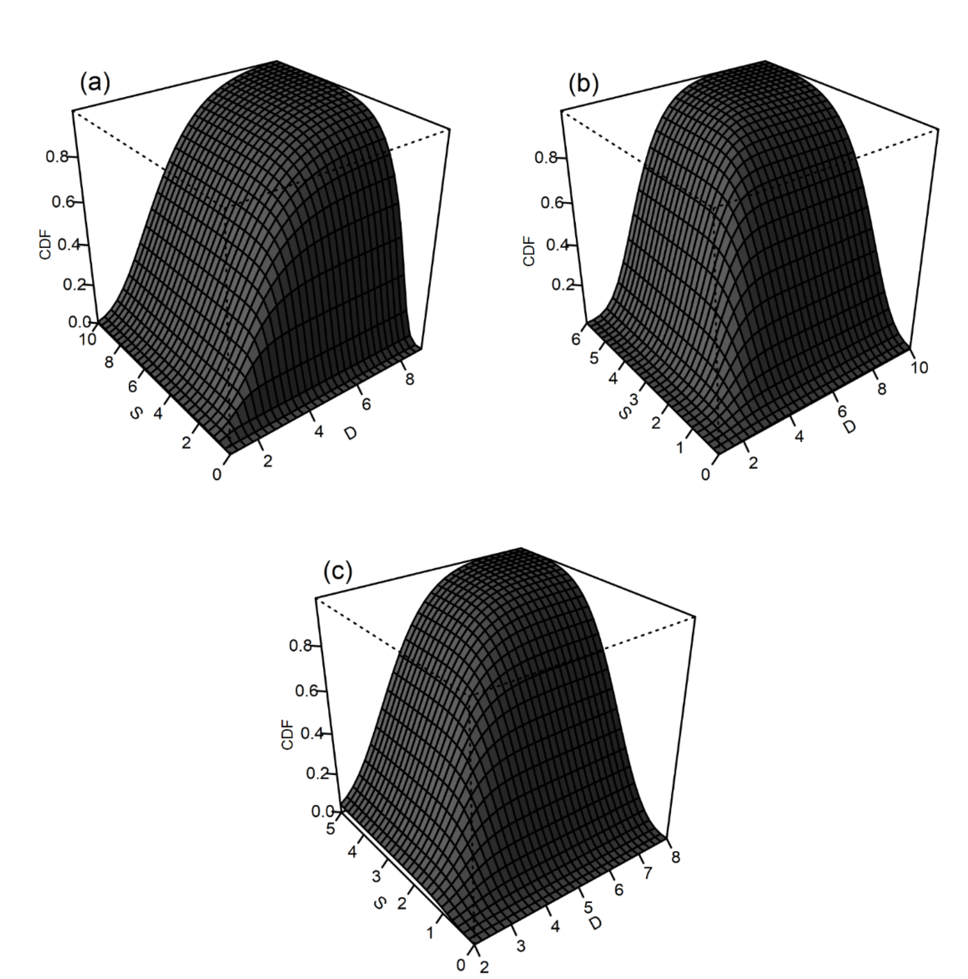A series of HD indicators, such as streamflow drought index (SDI) and standardized runoff index (SRI), have been developed to quantitatively assess the severity of hydrological drought [13,14]. In addition, given the fact that a drought event generally has multiple attributes such as duration and severity, researchers are more inclined to study the relationship between those attributes and their joint risk levels to provide comprehensive characterization for drought events [15,16]. Due to the flexibility of establishing marginal and joint distributions, copula-based methods are widely used in joint risk inferences for droughts in a multivariate context in recent years [17,18,19,20].

Hydrological drought can indicate the natural decline of water resources compared to past records. However, it cannot reflect the pressure of water scarcity (WS). Therefore, it is necessary to adopt appropriate methods to identify and assess the WS or water stress conditions. Numerous indicators have been developed to help identify and characterize water scarcity areas across the globe. These indicators include, for example, the ratio of water withdrawal or population size to renewable water, and the ratio of water demand or water consumption to available water [21,22,23,24]. Among these indicators, Water Exploitation Index (WEI) is widely used to describe the WS status in European Union countries [2,24,25]. WEI evaluates the ratio of total annual freshwater extraction to long-term average renewable resources, and addresses pressure on water resources from all water sectors in the study area. Rather than concentrating on the annual average WS and mainly used in national scale for the WEI, the more advanced Water Exploitation Index Plus (WEI+) takes into account the water return component and has been given more attention in studying the interannual changes in WS of river basins [26,27,28].

Although there are numerous studies on HD, there is a lack of research on the future multivariate risk of HD under climate change. In addition, the study of WS often requires a large amount of hydrological data, especially for the river basins across many administrative regions, which limits the study of WS (including future WS) in data-lacked watersheds. HD and WS can, respectively, reflect the degree of water shortage from the perspective of nature and human demand. 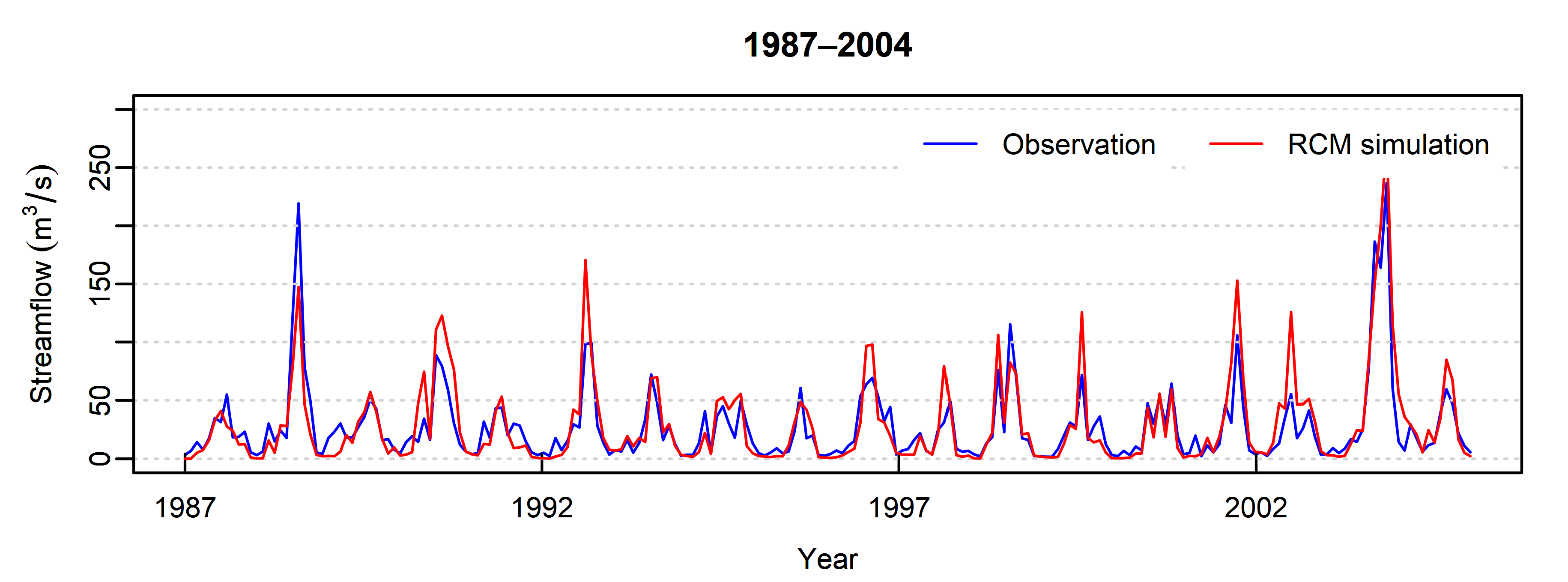It should be noted that the assessment of WS may be over optimistic if only the richness of future water resources is adopted based on drought indicators without considering water use factors [29]. Therefore, it is extremely important to comprehensively assess the possible development trend of HD and WS in the future. In recent years, the methods of coupling regional climate model (RCM) and hydrological model are widely used to simulate the future runoff of river basins [30,31,32]. For example, Hurkmans et al. [30] and Wan et al. [31] have applied bias-corrected RCM outputs to drive hydrological models and produce runoff series under different Representative Concentration Pathway (RCP) scenarios in the future. These studies provide good pathways for studying the HD and WS in the future.

The main purpose of this study is to establish a modeling framework, which allows us to estimate the multivariate risk of HD variables, and also provide quantitative analyses for WS. In detail, the constructed model framework contains the following modules to achieve these goals: (i) a combined climate and hydrological system to project future runoff under different climate scenarios; (ii) a copula-based model for multivariate risk assessment of HD; (iii) the WEI+ indicator to estimate future WS. The developed modeling framework is applied to Jinghe River Basin (JRB) of China. The univariate and bivariate risk of HD variables and the WS degrees in various water consumption scenarios will be obtained over the JRB under climate change. The comprehensive evaluation results of HD and WS can help decision-makers to make perspective long-term water use plans and take measures to reduce losses that may be caused by drought in the future.

2. Study Area and Data

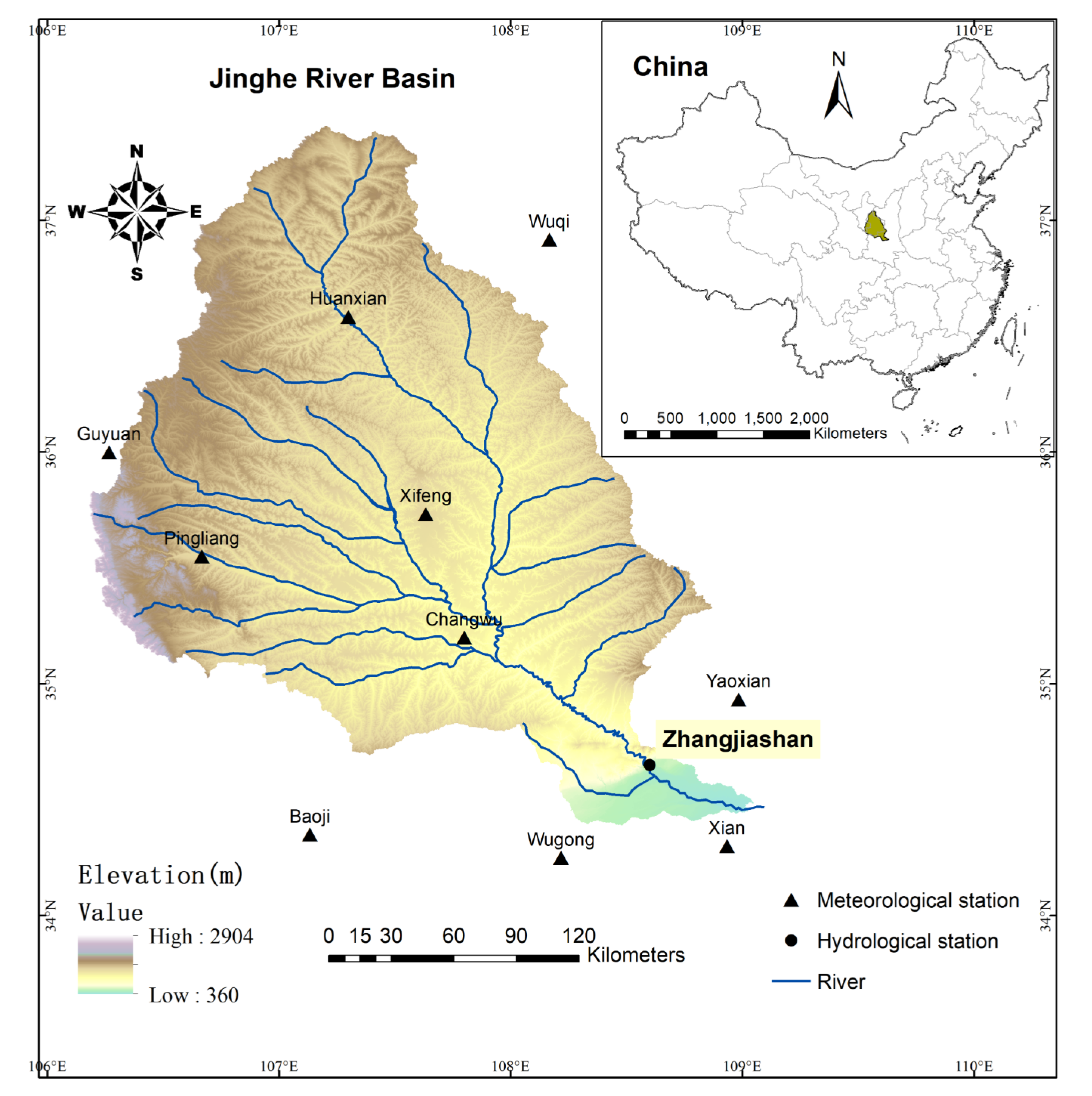
The Jinghe River Basin (JRB, lies between 34°46′ N to 37°19′ N and 106°14′ E to 108°42′ E) is located in the central part of Loess Plateau in China (Figure 1), with a total drainage area of 45,412 km². The JRB flows across three provinces (Ningxia, Gansu and Shanxi) from northwest to southeast, and has a typical temperate continental climate. The annual average temperature in JRB ranges between 8 and 10 ℃, and the average annual precipitation varies from 350 to 650 mm. Frequent droughts coupled with over-exploitation of water resources have caused serious water shortages in this area.

Observed daily meteorological data of precipitation, maximum temperature (Tmax), minimum temperature (Tmin), and wind speed with time period of 1960–2009 at 10 meteorological stations (located in and around the JRB, Figure 1) were obtained from the China Meteorological Administration. Gridded regional climate model data (RegCM driven by GFDL-ESM2M global climate model outputs [33,34,35]) of daily precipitation, Tmin, Tmax and wind speed at a 0.44-degree resolution under historical (1985–2004) and future periods (2020–2099 under scenarios of RCP4.5 and RCP8.5) were collected from China Climate Change Data Portal (http://chinaccdp.org/). The climate projections are bias-corrected using the Quantile Mapping method [36], and all climate data are interpolated to a resolution of 0.22 degrees through the Inverse Distance Weighted (IDW) interpolation method [37].

Observed daily runoff data of 1960–2009 at Zhangjiashan hydrometric station (Figure 1) were obtained from the National Earth System Science Data Center (http://loess.geodata.cn/). The annual runoff, annual renewable water and water resources changes between 2000 and 2017 were obtained from Water Resources Bulletins of Ningxia, Gansu, and Shaanxi provinces. Three categories of geographic information data were used for the hydrological model: the digital elevation model data with 90 m resolution were collected from the Shuttle Radar Topography Mission (SRTM); the land cover data at 1 km resolution were achieved from the Global Land Cover Production of University of Maryland [38]; the soil type data at 30 arc second resolution were collected from Food and Agriculture Organization [39].

3. Methods

3.1. Runoff Simulation and Drought Identification

In this study, the climate projections (2020–2099) are employed to drive the Variable Infiltration Capacity (VIC) model [40,41] to obtain future runoff for two RCP scenarios. The VIC hydrological model is run at a 0.22-degree resolution (24-h time scale), and then the runoff and base flow of the simulated grid cells are processed by a river routing model [42]. Detailed information for the VIC model can be found in Zhang et al. [43]. The VIC model is calibrated for the period of 1981–1990 and validated for the period of 1998–2005 before being used to generate future runoff. The performance of the VIC model is assessed by the Nash–Sutcliffe efficiency coefficient (NSE, Equation (1)) [44,45] and determination coefficient (R², Equation (2)).

$$NSE=1-\frac{{\displaystyle \sum _{i=1}^N{(Q_{mod,i}-Q_{obs,i})}^2}}{{\displaystyle \sum _{i=1}^N{(Q_{obs,i}-\overline{Q_{obs}})}^2}}$$

(1)

$$R^2=\frac{{\left[{\displaystyle \sum _{i=1}^N(Q_{obs,i}-\overline{Q_{obs}})(Q_{mod,i}-\overline{Q_{mod}})}\right]}^2}{\left[{\displaystyle \sum _{i=1}^N{(Q_{obs,i}-\overline{Q_{obs}})}^2}\right]\left[{\displaystyle \sum _{i=1}^N{(Q_{mod,i}-\overline{Q_{mod}})}^2}\right]}$$

(2)

where $Q_{obs,i}$ and $Q_{mod,i}$ are the observed and modeled streamflows for month i respectively; $\overline{Q_{obs}}$ and $\overline{Q_{mod}}$ represent the monthly mean observed and simulated streamflows, respectively; N is the length of data. To evaluate the reliability of streamflow simulations driven by the outputs from RegCM, the historical projections (1986–2004) of RegCM are then used to drive the validated VIC model, and the generated runoff simulations (1987–2004) are compared with the runoff from the gridded observations. The historical simulations of the first year (1986) are removed in the validation process because the VIC model has an adaptation process during operation.

It is worth noting that the simulation results of annual runoff volume are needed in the subsequent calculation process of WEI+. Although NSE and R2 can well reflect the fluctuation of monthly runoff time series, they cannot reflect the deviation degree of runoff volumes. Therefore, the deviation of the runoff volumes (DV, [46]) indicator is then calculated. The closer the DV value is to 1, the smaller the volumetric deviation is:

$$DV=\frac{{\displaystyle {\sum }_{t=1}^n{V}_{sim}}}{{\displaystyle {\sum }_{t=1}^n{V}_{obs}}}$$

(3)

where $V_{obs,t}$ and $V_{sim,t}$ represent the observed and simulated annual runoff volumes in year t, respectively; n is the number of the data.

The SDI is used to identify hydrological drought events and their corresponding characteristics (duration and severity). SDI can be calculated from monthly streamflows:

$$V_{i,j}=Q_{i,j}+Q_{i,j-1}+\cdots +Q_{i,j-m+1}\begin{array}{cc}\begin{array}{c}\end{array}i=1,2,\dots & j=1,2,\dots ,12\end{array}$$

(4)

where m is the time scale (can be 1, 3, 6, 12 et al.); $Q_{i,j}$ is the runoff in month j, year i; $V_{i,j}$ denotes the cumulative streamflow of the chosen time scale. The SDI values can be obtained by normalizing the $V_{i,j}$ values [13]:

$$SD{I}_{i,j}=\frac{V_{i,j}-\overline{V}}{s_V}$$

(5)

where $\overline{V}$ and $s_V$ represent the average and standard deviation of $V_{i,j}$, respectively. The thresholds of HD according to SDI values are shown in

Table 1. Thresholds of HD and WS based on SDI [13] and WEI+, respectively.

SDI	HD Level	WEI+	WS Level
>0	Non	<0.1	No stress
−1.0–0	Mild	0.1–0.2	Low stress
−1.5–−1.0	Moderate	0.2–0.3	Moderate stress
−2.0–−1.5	Severe	0.3–0.4	Scarcity
<−2.0	Extreme	>0.4	Sever scarcity

HD: hydrological drought; SDI: streamflow drought index; WS: water scarcity; WEI+: Water Exploitation Index Plus.

[13]. In this study, duration and severity of HD events are derived from monthly SDI values using the threshold approach [47,48,49]. The duration of a HD event is the time period from the beginning to the end of the event, and severity is the cumulative deviation of the SDI below the threshold. More details of HD identification process and HD duration and severity meanings are presented in Figure S1 and its explanations in the Supplementary Materials.

3.2. Multivariate Hydrological Drought Risk

3.2.1. The Copula Method

In reality, duration and severity of HD events are correlated with each other. An individual variable (duration or severity) of the HD event can hardly provide the event a comprehensive description and thus may lead to misestimation of the HD risk. Therefore, the correlation between HD variables should be carefully taken into account in HD risk analysis. Developed by Sklar [50], copulas can be used to construct multivariate distributions in a flexible way in choosing marginal distributions and their dependence structures [51,52]. A two-dimensional copula function can be expressed as:

$$F(x,y)=C(F_X(x),F_Y(y))$$

(6)

where (F_X, F_Y) represent the cumulative distribution functions (CDFs) of a two-dimensional random vector (X, Y).

Marginal distributions are fitted for the variables before establishing the bivariate distribution in Equation (6). Gamma, lognormal (LN), Weibull, generalized extreme value (GEV), Pearson type III (P-III), and Log Pearson type III (LP III) distributions are employed to establish marginal distributions for HD variables. The goodness-of-fit tests for marginal distributions are implemented by using the Akaike’s information criteria (AIC) [53], root mean square error (RMSE) and Kolmogorov–Smirnov (KS) statistic test [54].

Because of the simplicity and good accuracy properties, Archimedean copulas have attracted wide attention in drought risk analyses [15,55]. Three Archimedean copulas: Frank, Clayton, and Gumbel–Hougaard are chosen as candidate models to derive bivariate distribution for the duration and severity of HD events. The parameters in the chosen copulas are obtained through the method-of-moments-like (MOM) estimator [56]. The Cramér-von Mises statistic (CvM) test [57], AIC and RMSE are used for goodness-of-fit tests of copulas.

3.2.2. Drought Risk Analysis

In this study, different kinds of return periods are adopted to quantify the risk of drought events. The return period is the mean interval time between two consecutive drought events. The univariate return periods of the two HD variables can be derived by estimating the exceedance probability from the fitted marginal distributions:

$$T_D=\frac{E(L)}{1-F_D(d)}$$

(7)

$$T_S=\frac{E(L)}{1-F_S(s)}$$

(8)

where T_D/T_S denotes the return period of duration (D)/severity (S) larger than d/s; E(L) represents the average interarrival time of the HD variable; F_D(d) and F_S(s) are CDFs of duration and severity, respectively. Two types of joint return periods (JRPs) are considered in this study to quantitatively evaluate the joint risk of the two variables:

$$\begin{array}{l}{T}_{DS}^{AND}=\frac{E(L)}{P(D\ge \mathrm{d},S\ge d)}=\frac{E(L)}{1-F_D(d)-F_S(s)+F_{DS}(d,s)}\\ \begin{array}{cc}& \end{array}=\frac{E(L)}{1-F_D(d)-F_S(s)+C(F_D(d),F_S(s))}\end{array}$$

(9)

$$T_{DS}^{OR}=\frac{E(L)}{P(D\ge \mathrm{d} \mathrm{or} S\ge d)}=\frac{E(L)}{1-F_{DS}(d,s)}=\frac{E(L)}{1-C(F_D(d),F_S(s)))}$$

(10)

where $T_{DS}^{AND}$ denotes the JRP when D and S respectively exceed specific values of d and s; $T_{DS}^{OR}$ denotes the JRP when D or S is higher than the certain thresholds (i.e., D ≥ d or S ≥ s). F_DS(d,s) is the joint CDF of D and S.

3.3. Water Exploitation Index +

The WS indicator used in this study is the WEI+. It is applied to analyze the level of pressure exerted by human activities on natural water resources. WEI+ is calculated as the ratio of water withdrawal minus return water (i.e., net water consumption, in m³) and renewable water resources (in m³) [26,27]:

$$\mathit{WEI}+=(Abstractions-Returns)/\mathit{RWR}$$

(11)

where Abstractions refers to the total water resources extracted from the watershed (containing surface and ground water); Returns indicates the amount of water resources that have been exploited and re-entered into the hydrological cycle; RWR is the amount of renewable water resources. For basins influenced by human activities, two methods exist for renewable water calculation [26]:

$$\mathrm{Method} 1\text{:} \mathit{RWR}=E\mathrm{x}In+P-Eta-\Delta S_{nat}$$

(12)

$$\mathrm{Method}2\text{:} \mathit{RWR}=Outflow+(Abstractions-Returns)-\Delta S_{\mathrm{art}}$$

(13)

where ExIn (External Inflow) indicates the amount of surface water and groundwater inflow from outside the basin; P refers to the total precipitation; Eta (Evapotranspiration) denotes the total evapotranspiration; $\Delta S_{nat}$ refers to the change of water resources reserves in natural environment; Outflow refers to the actual water resources flowing out of the drainage basin; $\Delta S_{art}$ denotes changes in water reserves in artificially regulated lakes or artificial reservoirs. Thresholds of water stress according to the WEI+ are shown in Table 1 [27,58].

4. Results Analysis

4.1. Hydrological Model Verification and Hydrological Drought Identification

The NSE and R² calculated from monthly flow discharges are 0.80 and 0.86, respectively, for the calibration period 1981–1990, and are 0.78 and 0.82, respectively, for the validation period of 1998–2005. These indicate that the runoff simulations and observations are in good agreement. Figure 2 shows the comparison between the monthly runoff simulated from climate model projections and from the gridded observations of 1987–2004 (with NSE and R² are 0.71 and 0.78, respectively). The simulated and observed annual runoff volumes produce an DV value of 1.04, which is very close to 1. All these indicate that the simulated runoff series driven by the outputs of RegCM perform well in capturing the runoff variations in observations, and thus the future runoff simulations can then be used for HD- and WS-related calculations.

The monthly streamflow series of observations from 1960 to 2009 and projections from 2020 to 2099 are used to generate the SDI values for both history and two future scenarios. The SDI variations with corresponding monthly precipitation series under history and projected future scenarios are depicted in Figure 3, which helps understand the runoff deficit under different precipitation conditions. The average annual precipitation under RCP4.5 and RCP8.5 scenarios would increase by 108.1 mm and 135.9 mm respectively compared with that in the historical period. The SDIs over the historical period changes from −3.46 to 3.44, and SDIs under scenarios of RCP4.5 and RCP8.5 have ranges of [−1.75, 5.45] and [1.46, 4.06], respectively. The mean values of SDIs for RCP4.5 and RCP8.5 are, respectively, 0.29 and 0.33 higher than those in the historical period. We can preliminarily conclude that hydrological droughts would be relieved under projected future climate change scenarios.

HD events with their corresponding deficit characteristics (duration and severity) are identified from monthly SDI series.

Table 2. Statistical information on duration (D) and severity (S) of hydrological drought events in different time periods.

Scenarios	Happen Times	Mean Interval (month)	Mean D (month)	Max D (month)	Mean S	Max S	Kendall τ between D&S
History	50	12	3.84	7	2.05	7.97	0.6262
RCP 4.5	75	12.96	3.71	8	1.89	4.98	0.6722
RCP 8.5	69	14.08	3.68	6	1.82	3.67	0.6012

provides the statistical information about the characteristics of HD occurrence, persistence and severity under history and two projected future scenarios. Mean interval time of HD events would be increased by 0.96 and 2.08 months in RCP4.5 and RCP8.5, respectively. Average HD duration and severity for projected future scenarios would slightly decrease when compared with those in the historical period. The maximum value of severity for historical HD events is 7.97 and it would be respectively reduced to 4.98 for RCP4.5 and 3.67 for RCP8.5. The Kendall correlation coefficient (τ) [19] between drought duration and severity under historical and future scenarios ranges from 0.60 to 0.67, which indicates that there is a strong correlation between the two variables.

4.2. Hydrological Drought Risk Analyses

4.2.1. Univariate and Bivariate Distributions

The univariate distributions for HD variables are achieved based on the identified HD records in both historical and future periods.

Table 3. Goodness-of-fit tests for fitted distributions of HD duration and severity.

Scenarios	Drought Variables	Marginal Distribution	a	b	α	KS Test		RMSE	AIC
						T	p-Value
History	Duration	Gamma	5.65	0.68	–	0.0763	0.9117	0.0243	−367.6411
	Severity	LN	0.51	0.59	–	0.0626	0.9826	0.0199	−387.7808
RCP4.5	Duration	GEV	−0.1	1.02	3.23	0.0561	0.962	0.0212	−572.2235
	Severity	GEV	−0.07	0.83	1.44	0.073	0.7921	0.0272	−534.615
RCP8.5	Duration	GEV	−0.17	0.98	3.26	0.0593	0.9567	0.0187	−542.9995
	Severity	Weibull	2.43	2.07	–	0.0538	0.9821	0.0232	−515.111

Notes: Parameters of marginal distribution functions of HD variables: a, b and α indicates the shape, scale and location parameter, respectively.

shows the parameters of AIC, RMSE and KS test results for the best fitted distributions for HD duration and severity. It can be seen that the Gamma and LN distributions would be employed for HD duration and severity in a historical period. The GEV distribution is suitable for both HD duration and severity under the RCP4.5 scenario. The HD duration and severity under the RCP8.5 scenario are fitted with GEV and Weibull distributions, respectively. The p-values of the KS test results for all fitted distributions are greater than 0.05, which indicate that these distributions can effectively describe the probability characteristics of the HD variables. Figure 4 illustrate the comparison of empirical and theoretical CDFs for HD duration and severity under historical period and projected future scenarios. It shows that the theoretical CDFs from best fitted distributions of the HD variables are very close to empirical distributions.

The dependence structure between HD duration and severity is then characterized by the copula functions.

Table 4. Goodness-of-fit tests of best fitted copulas for HD duration and severity under historical periods and projected future scenarios.

Scenarios	Copulas	Parameter	RMSE	AIC	CvM	p-Value
History	Clayton	2.9595	0.0180	−399.9048	0.0220	0.5149
RCP4.5	Gumbel	2.2783	0.0259	−546.2171	0.0162	0.7040
RCP8.5	Frank	5.9656	0.0186	−548.0859	0.0205	0.5249

shows the statistical test results for best fitted copulas. The Clayton, Gumbel and Frank copulas are, respectively, the best choices in modeling the joint distributions of HD duration and severity under history and two future scenarios. Figure 5 displays the bivariate CDFs based on the fitted copulas for HD duration and severity under history and two future scenarios.

4.2.2. Return Periods of Hydrological Drought Events

Six return period levels from 3 to 100 (in Figure 6) for HD duration and severity are estimated according to Equations (7) and (8). Figure 6 shows that the values of the two variables for all return periods in both future scenarios would decrease significantly, especially in the RCP8.5 scenario. Under the RCP4.5 scenario, the 3-year and 100-year return periods of HD duration would reduce by 0.28 and 1.54 months, respectively, compared with those in the historical stage, and they would decrease by 0.4 months and 2.2 months, respectively, under the RCP8.5 scenario. The severity of drought with the same return periods would also decrease by 0.15 and 1.19 months under the RCP4.5 scenario, and by 0.22 and 2.07 months under the RCP8.5 scenario, respectively. These imply that HD events in the JRB would be significantly reduced under projected future scenarios.

For the reason that different combinations of HD variables can lead to the same JRP, the JRPs for two variables in the historical period and future scenarios calculated by Equations (9) and (10) are shown in the contour plots in Figure 7. The JRPs at six levels (3, 5, 10, 20, 50, 100 years) for historical period and projected future scenarios are quite different. According to the contour plots, once certain values of HD variables are given (

Table 5. Joint return periods for hydrological drought events at given duration and severity in Figure 6.

Return Period	Tand (Years)			Tor (Years)
	History	RCP4.5	RCP8.5	History	RCP4.5	RCP8.5
3	4.00	4.04	4.12	2.40	2.39	2.36
5	7.95	8.08	8.32	3.65	3.62	3.57
10	22.38	22.92	23.89	6.44	6.40	6.32
20	70.50	72.64	76.54	11.65	11.60	11.50
50	368.02	381.38	405.79	26.82	26.75	26.64
100	1373.94	1427.37	1524.99	51.89	51.82	51.70

), the corresponding JRPs are much larger in future scenarios than that in the historical period. For example, when s is 2.8 and d is 5.5 in Figure 7a, the Tand for the historical period and projected RCP4.5 scenario are 10 and 20 years, respectively. This means that, with the same JRP, the future HD events would become less serious than those in historical situations.

4.3. Water Scarcity in the Jinghe River Basin

The Jinghe River flows across three provinces of Ningxia, Gansu, and Shanxi. The annual renewable water resources produced by the JRB and the changes in water availability in major artificial reservoirs (for 2000–2017, in m³) are obtained from the Water Resources Bulletins of the three provinces. The annual net water consumption can be evaluated according to Equation (13), and the annual WEI+ of the watershed can then be obtained based on Equation (8). The WEI+ of the JRB from 2000 to 2017 are shown in

Table 6. The WEI+ from 2000 to 2017 for the JRB.

Year	2000	2001	2002	2003	2004	2005	2006	2007	2008
WEI+	0.54	0.56	0.57	0.42	0.58	0.55	0.67	0.67	0.70
Year	2009	2010	2011	2012	2013	2014	2015	2016	2017
WEI+	0.72	0.48	0.50	0.64	0.55	0.64	0.69	0.74	0.67

. The average annual net water consumption in 2000–2008 is 881 million m³ and the average WEI+ is 0.59. The average annual net water consumption in 2009–2017 is 1093 million m³, and the average WEI+ is 0.62. Water consumption has increased significantly in these 9 years, while the increase in WEI+ is not visible, which may be due to precipitation increases during these years in the JRB.

With the development of our socio-economic society, water consumption is expected to increase continuously in the future [2]. To investigate possible conditions of WS in the future and explore the ultimate carrying capacity of water resources in the JRB, five water consumption scenarios for the future are set: the future water consumption is equivalent to the averaged water consumption in the past nine years (2009–2017), denoted as S0; the water consumption at the end of the century is 10%, 20%, 30% and 40% higher than that in the past 9 years and has a constant increasing rate for every ten years, which are respectively denoted as S1, S2, S3 and S4. The fluctuation of water reserves in the artificial reservoir is set to be zero since it has very little impact on the total water resources. The WEI+ values for the five water consumption scenarios under climate change projections of RCP4.5 and RCP8.5 are then calculated. The frequencies of WEI+ located in different intervals for each scenario are shown in

Table 7. Frequencies of WEI+ located in different intervals for each scenario.

Scenarios	Schemes	<0.4	0.4–0.5	0.5–0.6	0.6–0.7	0.7–0.8	0.8–0.9	0.9–1	>1
Happen times of RCP4.5	S0	2	4	14	21	31	6	2	0
	S1	1	3	13	20	29	11	2	1
	S2	0	2	10	16	26	20	5	1
	S3	0	2	6	16	24	19	11	2
	S4	0	1	6	11	22	22	12	6
	Mean	0.6	2.4	9.8	16.8	26.4	15.6	6.4	0.6
Happen times of RCP8.5	S0	2	17	12	21	15	12	0	0
	S1	1	14	10	15	24	13	1	1
	S2	0	10	13	14	16	23	2	1
	S3	0	5	15	13	14	24	5	2
	S4	0	7	13	10	14	18	15	6
	Mean	0.6	10.6	12.6	14.6	16.6	18	4.6	2

.

Table 7 shows that the WEI+ would be most frequently located in the interval 0.7 to 0.8 under the five water consumption scenarios, with an average of 26.4 times under RCP4.5 and 16.6 times under RCP8.5. The values of WEI+ from S0 to S5 under the RCP4.5 scenario are mainly concentrated (occupied 73.5%) in the interval of [0.6, 0.9]. While the values of WEI+ are more dispersedly distributed between 0.4 and 0.9 under RCP8.5, indicating that the water pressure will vary significantly under this scenario. For the extreme scenario of S4, the WEI+ greater than 1 would be observed on six occasions under both climate change scenarios, which means that non-renewable water is available or water resources may need to be imported from outside to meet the demand in some years. The 10-year average WEI+ is applied to reflect the water pressure fluctuations at different time periods under different scenarios in the future (

Table 8. The 10-year average WEI+ corresponding to different intervals for each scenario.

Scenarios	Schemes	20–29	30–39	40–49	50–59	60–69	70–79	80–89	90–99
Mean value of WEI+ for RCP4.5	S0	0.74	0.71	0.65	0.74	0.65	0.61	0.64	0.62
	S1	0.74	0.72	0.67	0.77	0.69	0.65	0.70	0.69
	S2	0.74	0.73	0.69	0.81	0.73	0.70	0.75	0.75
	S3	0.74	0.74	0.71	0.84	0.77	0.74	0.80	0.81
	S4	0.74	0.76	0.73	0.87	0.80	0.78	0.86	0.87
	Mean	0.74	0.73	0.69	0.81	0.73	0.70	0.75	0.75
Mean value of WEI+ for RCP8.5	S0	0.70	0.64	0.61	0.66	0.63	0.64	0.53	0.59
	S1	0.70	0.65	0.63	0.68	0.67	0.69	0.58	0.65
	S2	0.70	0.65	0.65	0.71	0.71	0.73	0.62	0.71
	S3	0.70	0.66	0.67	0.74	0.74	0.78	0.67	0.77
	S4	0.70	0.67	0.68	0.77	0.78	0.83	0.71	0.83
	Mean	0.70	0.65	0.65	0.71	0.71	0.73	0.62	0.71

). The values of WEI + at the end of the century under S3 and S4 scenario for RCP4.5 and S4 scenario for RCP8.5 are all greater than 0.8, which indicate that serious WS would occur at the end of the century. The WEI+ averages of S0–S4 in each time period show that the most severe WS under the RCP4.5 scenario is from 2059 to 2069, and the corresponding mean value of WEI+ is 0.81.

According to the classification of water resources pressure shown in Table 1, severe WS occurs when WEI+ exceeds 0.4, and some researchers believe that the freshwater ecosystems of a river basin cannot be healthily maintained in this state [26,27]. However, some studies argue that the utilization rate of water resources can be greatly improved, and thus a threshold of 0.6 would be a more appropriate value [27]. Although it requires further in-depth investigation to set the threshold, according to the comprehensive results of this study, the JRB will still be in a state of extreme WS for a long time under the projected future scenarios, even with a significant increase in precipitation.

5. Conclusions and Discussions

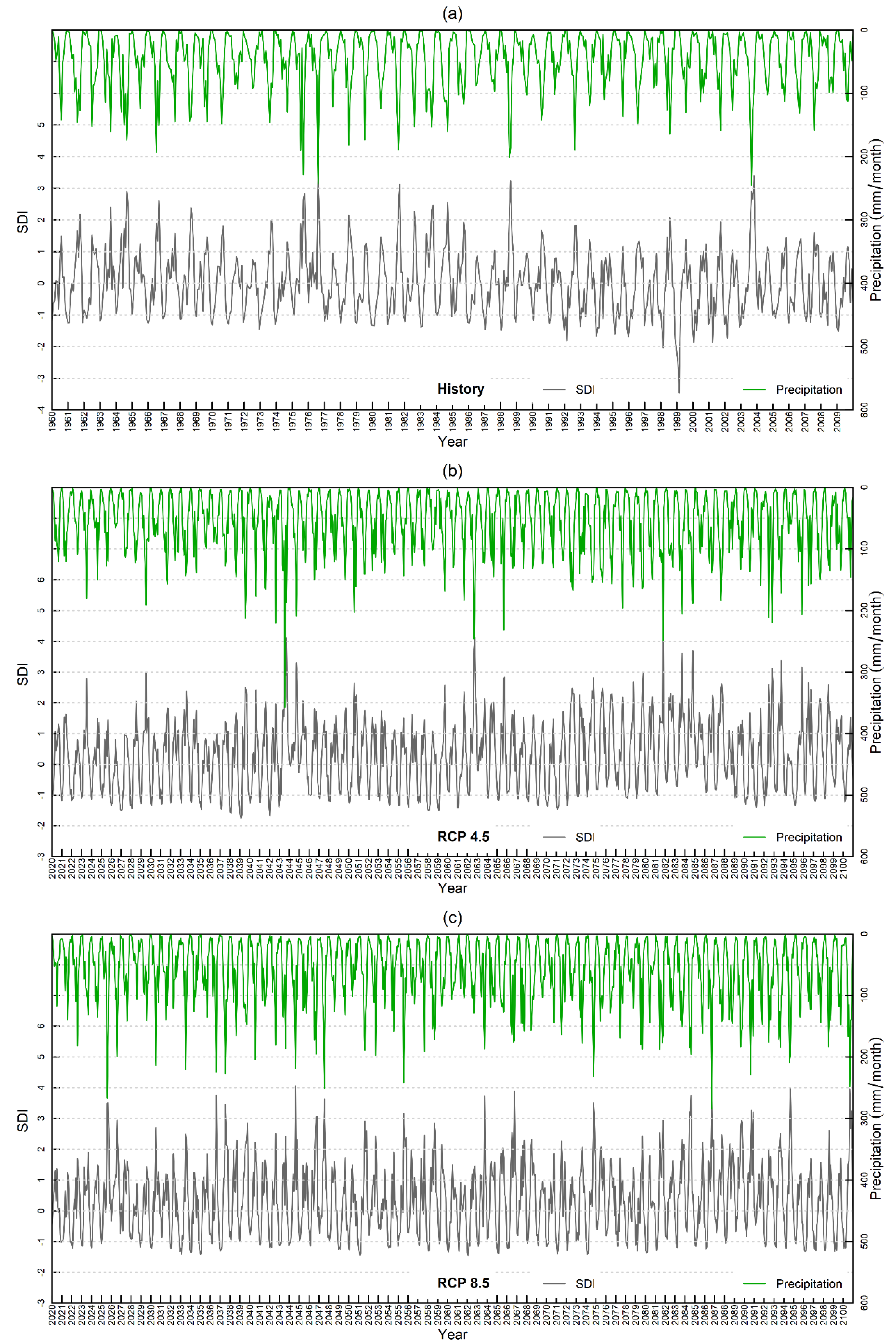
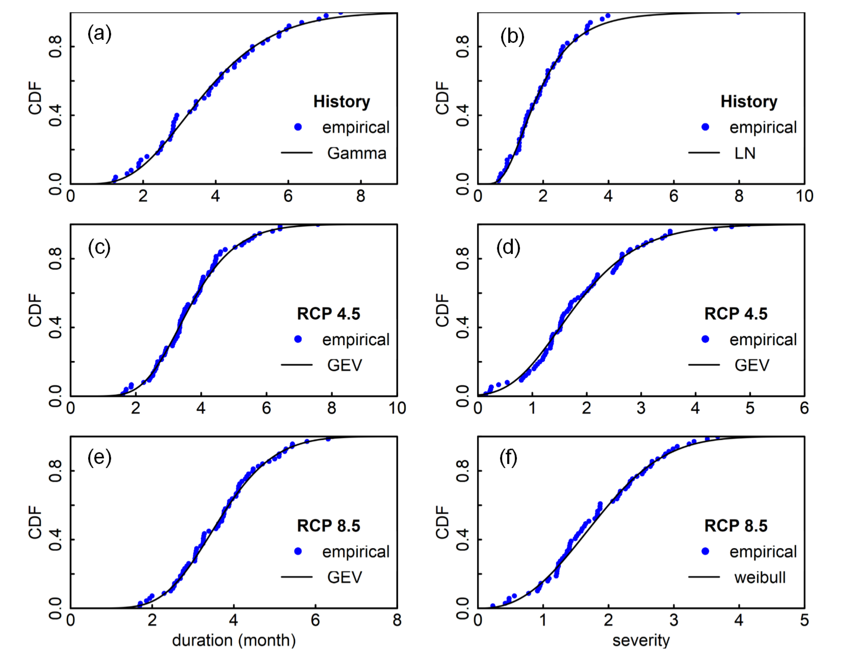
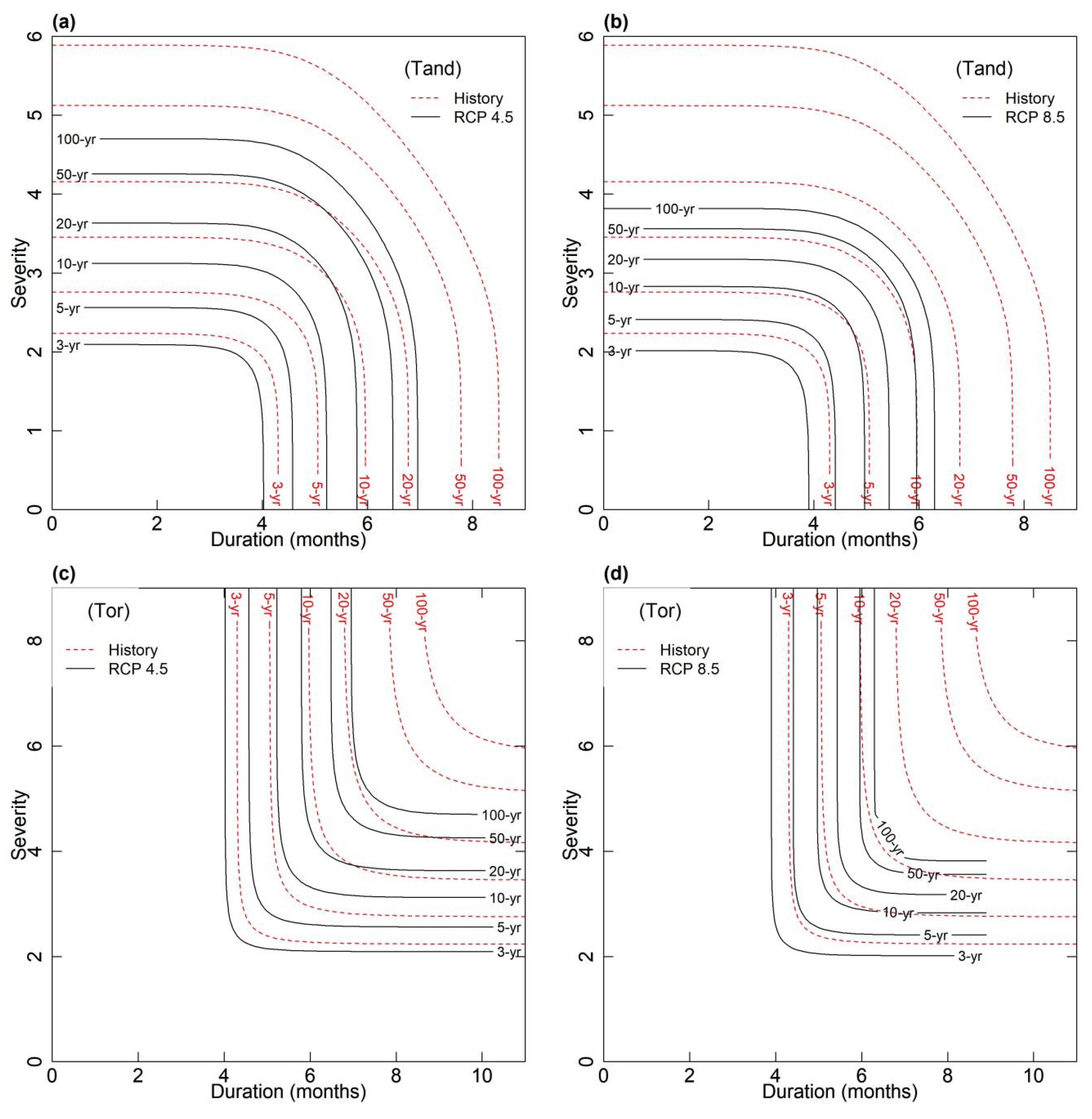
The presented modeling framework in this study allows us to estimate the univariate and joint risks of hydrological drought variables, and also provide quantitative analyses for water scarcity under climate change. The WEI+ index was innovatively applied to evaluate water scarcity in an arid basin (JRB) of China under climate change. Lower frequency with lower mean duration and severity of HD events were identified under RCP8.5 scenario than those characterized under the RCP4.5 scenario. HD duration and severity under both RCP scenarios are projected to decrease remarkably when compared to those in the past. The copula-based bivariate HD risk assessment model also reveals that climate change under projected future scenarios would alleviate drought situation in the JRB. However, the WS assessment results show that the shortage of water resources in JRB is still severe in the future.

Drought indicators can flexibly evaluate the degree of water resources deviating from normal at different time scales, such as the monthly SDI estimated in this study. The developed modeling framework has important implications for HD risk management. However, drought assessment can only reflect the relative changes of water resources in a natural state, without taking into account water consumption changes in the future. Therefore, simply assessing the severity of future droughts cannot accurately reflect the severity of water shortages, and decision-makers cannot provide valuable water resources management policies. Considering the increase in human water consumption in the future, the degree of water shortage may not be alleviated by the increase in precipitation and water availability. This makes it necessary to introduce quantitative assessment methods for future water scarcity evaluation.

Although setting thresholds for the WEI+ is still debatable, the authors suggest that the WEI+ thresholds for the basin should be set based on different environmental protection objectives and economic development goals. Moreover, an obvious disadvantage of the WEI+ indicator is the lack of consideration of water quality, which is closely related to the quality of “return water” (exploited and re-entered into the hydrological cycle). The WEI+ may be improved or different WS assessment methods can be used to comprehensively assess water stress and water quality in the future. However, a river basin often covers several provinces, and the conditions of water use are complex, which requires the relevant departments to do a more collaborative job on basic data statistics. The results of this study are of great significance for policy makers and local stakeholders to make a prospective long-term plan. Based on the assessment of future drought and water shortage status, an appropriate plan can be made to support the sustainable development of social economy. This research is repeatable and can be used in other basins in traditional arid or semi-arid areas. In addition, due to the increase in population and the acceleration of urbanization, the water shortages in large cities and their surrounding areas in some developed countries are becoming increasingly severe, and some water-rich countries have also experienced WS events in recent years. The presented modelling system can also be applicable in such areas.

References

1. Kossida, M.; Koutiva, I.; Makropoulos, C.; Monokrousou, K.; Mimikou, M.; Fons-Esteve, J.; Iglesias, A. Water Scarcity and Drought: Towards a European Water Scarcity and Drought Network (WSDN); European Environment Agency: Copenhagen, Denmark, 2009. [Google Scholar]
2. Van Loon, A.F.; Van Lanen, H.A.J. Making the distinction between water scarcity and drought using an observation-modeling framework. Water Resour. Res. 2013, 49, 1483–1502. [Google Scholar] [CrossRef]
3. Pedro-Monzonís, M.; Solera, A.; Ferrer, J.; Estrela, T.; Paredes-Arquiola, J. A review of water scarcity and drought indexes in water resources planning and management. J. Hydrol. 2015, 527, 482–493. [Google Scholar] [CrossRef] [Green Version]
4. FAO. Report of FAO-CRIDA Expert Group Consultation on Farming System and Best Practices for Drought-Prone Areas of Asia and the Pacific Region, Food and Agricultural Organisation of United Nations; Central Research Institute for Dry land Agriculture: Hyderabad, India, 2002. [Google Scholar]
5. World Bank. India, Financing Rapid Onset Natura Disaster Losses in India: A Risk Management Approach; Report No. 26844-IN; World Bank: Washington, DC, USA, 2003. [Google Scholar]
6. Berardi, U. Sustainable Water Use and Management—Examples of New Approaches and Perspectives; Springer: Heidelberg, Germany, 2015. [Google Scholar]
7. Dutra, E.; Magnusson, L.; Wetterhall, F.; Cloke, H.L.; Balsamo, G.; Boussetta, S.; Pappenberger, F. The 2010-2011 drought in the horn of africa in ecmwf reanalysis and seasonal forecast products. Int. J. Climatol. 2013, 33, 1720–1729. [Google Scholar] [CrossRef] [Green Version]
8. Masters, J. Top Ten Global Weather Events of 2012; Weather Underground: Ann Arbor, MI, USA, 2013; Available online: https://www.wunderground.com/blog/JeffMasters/top-ten-global-weather-events-of-2012.html (accessed on 8 April 2020).
9. Xie, Y.; Crary, D.; Bai, Y.; Cui, X.; Zhang, A. Modeling grassland ecosystem responses to coupled climate and socioeconomic influences in multi-spatial-and-temporal scales. J. Environ. Inf. 2019, 33, 37–46. [Google Scholar] [CrossRef]
10. FAO. Climate Change, Water and Food Security; FAO Water Reports No 36; Food and Agriculture Organization: Rome, Italy, 2011. [Google Scholar]
11. Gampe, D.; Nikulin, G.; Ludwig, R. Using an ensemble of regional climate models to assess climate change impacts on water scarcity in European river basins. Sci. Total Environ. 2016, 573, 1503–1518. [Google Scholar] [CrossRef]
12. Wilhite, D.A.; Glantz, M.H. Understanding the drought phenomenon: The role of definitions. Water Int. 1985, 10, 111–120. [Google Scholar] [CrossRef] [Green Version]
13. Nalbantis, I. Evaluation of a hydrological drought index. Eur. Water 2008, 23, 67–77. [Google Scholar]
14. Shukla, S.; Wood, A.W. Use of a standardized runoff index for characterizing hydrologic drought. Geophys. Res. Lett. 2008, 35, 226–236. [Google Scholar] [CrossRef] [Green Version]
15. Shiau, J.T. Fitting drought duration and severity with two-dimensional copulas. Water Resour. Manag. 2006, 20, 795–815. [Google Scholar] [CrossRef]
16. Mirabbasi, R.; Fakheri-Fard, A.; Dinpashoh, Y. Bivariate drought frequency analysis using the copula method. Theor. Appl. Climatol. 2012, 108, 191–206. [Google Scholar] [CrossRef]
17. Jaworski, P.; Härdle, W.K.; Rychlik, T.; Durante, F. Copula Theory and Its Applications. In Proceedings of the Workshop, Warsaw, Poland, 25–26 September 2009; Springer: Berlin/Heidelberg, Germany, 2010. [Google Scholar]
18. Fan, Y.R.; Huang, W.W.; Huang, G.H.; Huang, K.; Li, Y.P.; Kong, X.M. Bivariate hydrologic risk analysis based on a coupled entropy-copula method for the Xiangxi river in the Three Gorges Reservoir area, China. Theor. Appl. Climatol. 2016, 125, 381–397. [Google Scholar] [CrossRef]
19. Fan, Y.R.; Huang, W.W.; Huang, G.H.; Li, Y.P.; Huang, K.; Li, Z. Hydrologic risk analysis in the Yangtze river basin through coupling Gaussian mixtures into copulas. Adv. Water Resour. 2016, 88, 170–185. [Google Scholar] [CrossRef] [Green Version]
20. Sun, C.X.; Huang, G.H.; Fan, Y.; Zhou, X.; Lu, C.; Wang, X.Q. Drought occurring with hot extremes: Changes under future climate change on Loess Plateau, China. Earth’s Future 2019, 7, 587–604. [Google Scholar] [CrossRef] [Green Version]
21. Alcamo, J.; Henrichs, T. Critical regions: A model-based estimation of world water resources sensitive to global changes. Aquat. Sci. 2002, 64, 352–362. [Google Scholar] [CrossRef]
22. Viala, E. Water for food, water for life a comprehensive assessment of water management in agriculture. Irrig. Drain. Syst. 2008, 22, 127–129. [Google Scholar] [CrossRef]
23. Hoekstra, A.Y.; Mekonnen, M.M.; Chapagain, A.K.; Mathews, R.E.; Richter, B.D. Global monthly water scarcity: Blue water footprints versus blue water availability. PLoS ONE 2012, 7, e32688. [Google Scholar] [CrossRef]
24. Vanham, D.; Hoekstra, A.Y.; Wada, Y.; Bouraoui, F.; De Roo, A.; Mekonnen, M.M.; van de Bund, W.J.; Batelaan, O.; Pavelic, P.; Bastiaanssen, W.G.M.; et al. Physical water scarcity metrics for monitoring progress towards SDG target 6.4: An evaluation of indicator 6.4.2 “level of water stress”. Sci. Total Environ. 2018, 613, 218–232. [Google Scholar] [CrossRef]
25. EEA. Use of Freshwater Resources in Europe; European Environmental Agency: Copenhagen, Denmark, 2003; Available online: http://www.eea.europa.eu/data-and-maps/indicators/water-exploitation-index (accessed on 15 April 2020).
26. Faergemann, H. Update on Water Scarcity and Droughts Indicator Development; European Environment Agency: Copenhagen, Denmark, 2012. [Google Scholar]
27. Karabulut, A.; Egoh, B.N.; Lanzanova, D.; Grizzetti, B.; Bidoglio, G.; Pagliero, L.; Bouraoui, F.; Aloe, A.; Reynaud, A.; Maes, J.; et al. Mapping water provisioning services to support the ecosystem-water-food-energy nexus in the Danube River Basin. Ecosyst. Serv. 2016, 17, 278–292. [Google Scholar] [CrossRef]
28. Eurostat. Water Exploitation Index; European Commission: Brussels, Belgium, 2019; Available online: https://ec.europa.eu/eurostat/web/products-datasets/-/t2020_rd220 (accessed on 20 April 2020).
29. Gao, X.R.; Zhao, Q.; Zhao, X.N.; Wu, P.; Pan, W.X.; Gao, X.D.; Sun, M. Temporal and spatial evolution of the standardized precipitation evapotranspiration index (SPEI) in the Loess Plateau under climate change from 2001 to 2050. Sci. Total Environ. 2017, 595, 191–200. [Google Scholar] [CrossRef]
30. Hurkmans, R.; Terink, W.; Uijlenhoet, R.; Torfs, P.; Jacob, D.; Troch, P.A. Changes in streamflow dynamics in the rhine basin under three high-resolution regional climate scenarios. J. Clim. 2010, 23, 679–699. [Google Scholar] [CrossRef] [Green Version]
31. Wan, W.; Zhao, J.; Li, H.Y.; Mishra, A.; Wang, H. Hydrological drought in the anthropocene: Impacts of local water extraction and reservoir regulation in the U.S. J. Geophys. Res. Atmos. 2017, 122, 11313–11328. [Google Scholar] [CrossRef]
32. Wu, H.; Chen, B.; Snelgrove, K.; Lye, L.M. Quantification of uncertainty propagation effects during statistical downscaling of precipitation and temperature to hydrological modeling. J. Environ. Inform. 2019, 34, 139–148. [Google Scholar] [CrossRef]
33. Giorgi, F.; Coppola, E.; Solmon, F.; Mariotti, L.; Sylla, M.; Bi, X. RegCM: Model description and preliminary tests over multiple CORDEX domains. Clim. Res. 2012, 52, 7–29. [Google Scholar] [CrossRef] [Green Version]
34. Dunne, J.P.; Jasmin, G.J.; Shevliakova, E.; Stouffer, R.J.; Krasting, J.P. GFDL’s ESM2 global coupled climate-carbon earth system models. Part II: Carbon system formulation and baseline simulation characteristics. J. Clim. 2013, 26, 2247–2267. [Google Scholar] [CrossRef] [Green Version]
35. Shivam, G.; Goyal, M.K.; Sarma, A.K. Index-based study of future precipitation changes over subansiri river catchment under changing climate. J. Environ. Inform. 2019, 34, 1–14. [Google Scholar] [CrossRef]
36. Piani, C.; Weedon, G.P.; Best, M.; Gomes, S.M.; Viterbo, P.; Hagemann, S.; Haerter, J.O. Statistical bias correction of global simulated daily precipitation and temperature for the application of hydrological models. J. Hydrol. 2010, 395, 199–215. [Google Scholar] [CrossRef]
37. Willmott, C.J.; Rowe, C.M.; Philpot, W.D. Small-scale climate maps: A sensitivity analysis of some common assumptions associated with grid-point interpolation and contouring. Am. Cartogr. 1985, 12, 5–16. [Google Scholar] [CrossRef]
38. Hansen, M.C.; Defries, R.S.; Townshend, J.R.G.; Sohlberg, R.; Defries, R.S.; Belward, A.S. Global land cover classification at 1 km spatial resolution using a classification tree approach. Int. J. Remote Sens. 2000, 21, 1331–1364. [Google Scholar] [CrossRef]
39. Fischer, G.; Nachtergaele, F.; Prieler, S.; Velthuizen, H.T.V.; Verelst, L.; Wiberg, D. Global Agro-Ecological Zones Assessment for Agriculture (GAEZ 2008); Laxenburg, Austria and FAO: Rome, Italy, 2008. [Google Scholar]
40. Liang, X.; Lettenmaier, D.P. A simple hydrologically based model of land surface water and energy fluxes for general circulation models. J. Geophys. Res. 1994, 99, 415–428. [Google Scholar] [CrossRef]
41. Liang, X.; Lettenmaier, D.P.; Wood, E.F. One-dimensional statistical dynamic representation of subgrid spatial variability of precipitation in the two-layer variable infiltration capacity model. J. Geophys. Res. Atmos. 1996, 101, 21403–21422. [Google Scholar] [CrossRef]
42. Lohmann, D.; Raschke, E.; Nijssen, B.; Lettenmaier, D.P. Regional scale hydrology: I. Formulation of the VIC-2L model coupled to a routing model. Hydrol. Sci. 1998, 43, 131–141. [Google Scholar] [CrossRef]
43. Zhang, X.J.; Tang, Q.H.; Pan, M.; Tang, Y. A long-term land surface hydrologic fluxes and states dataset for china. J. Hydrometeorol. 2014, 15, 2067–2084. [Google Scholar] [CrossRef]
44. Nash, J.; Sutcliffe, J.V. River flow forecasting through conceptual models part I—A discussion of principles. J. Hydrol. 1970, 10, 282–290. [Google Scholar] [CrossRef]
45. Fan, Y.R.; Huang, G.H.; Baetz, B.W.; Li, Y.P.; Huang, K. Development of a copula-based particle filter (coppf) approach for hydrologic data assimilation under consideration of parameter interdependence. Water Resour. Res. 2017, 53, 4850–4875. [Google Scholar] [CrossRef] [Green Version]
46. Galván, L.; Olias, M.; Izquierdo, T.; Cerón, J.C.; Fernández de Villarán, R. Rainfall estimation in SWAT: An alternative method to simulate orographic precipitation. J. Hydrol. 2014, 509, 257–265. [Google Scholar] [CrossRef]
47. Yevjevich, V. An Objective Approach to Definitions and Investigations of Continental Hydrologic Droughts; Hydrology Papers; Colorado State University: Fort Collins, CO, USA, 1967. [Google Scholar]
48. Yuan, X.C.; Zhou, Y.L.; Jin, J.L.; Wei, Y.M. Risk analysis for drought hazard in china: A case study in Huaibei Plain. Nat. Hazards 2013, 67, 879–900. [Google Scholar] [CrossRef]
49. He, J.; Yang, X.; Li, Z.; Zhang, X.; Tang, Q. Spatiotemporal variations of meteorological droughts in China during 1961-2014: An investigation based on multi-threshold identification. Int. J. Disast. Risk Sci. 2016, 7, 63–67. [Google Scholar] [CrossRef] [Green Version]
50. Sklar, K. Fonctions dé repartition á n dimensions et leurs marges. Publ. Inst. Stat. Univ. Paris 1959, 8, 229–231. [Google Scholar]
51. Fan, Y.R.; Huang, G.H.; Huang, K. Uncertainty analysis for multivariate hydrologic risk in the Xiangxi River in Three Gorges Reservoir Area, China. Engineering 2018, 4, 617–626. [Google Scholar] [CrossRef]
52. Fan, Y.R.; Huang, G.H.; Li, Y.P.; Baetz, B.W.; Huang, K. Uncertainty characterization and partition in multivariate risk inference: A factorial Bayesian copula framework. Environ. Res. 2020, 183, 109215. [Google Scholar] [CrossRef]
53. Akaike, H. A new look at the statistical model identification. IEEE Trans. Autom. Control 1974, 19, 716–723. [Google Scholar] [CrossRef]
54. Frank, J.; Massey, J. The kolmogorov-smirnov test for goodness of fit. J. Am. Stat. Assoc. 1951, 46, 68–78. [Google Scholar]
55. Edoardo, B.; Georg, P.; Hall, J.W.; Stefan, H.S. Assessing water resource system vulnerability to unprecedented hydrological drought using copulas to characterize drought duration and deficit. Water Resour. Res. 2015, 51, 8927–8948. [Google Scholar]
56. Nelsen, R.B. An Introduction to Copulas; Springer: New York, NY, USA, 2006. [Google Scholar]
57. Genest, C.; Rémillard, B.; Beaudoin, D. Goodness-of-fit tests for copulas: A review and a power study. Insur. Math. Econ. 2009, 44, 199–213. [Google Scholar] [CrossRef]
58. EEA. The European environment—State and Outlook 2010: Synthesis; European Environment Agency: Copenhagen, Denmark, 2010. [Google Scholar]
Figure 1. Topography and the location of meteorological stations in the Jinghe River Basin.
Water 12 01605 g001
Figure 2. Monthly flow discharges (in m3/s) simulated from RCM projections and from the gridded observations over the Jinghe River basin for historical period of 1987–2004.
Water 12 01605 g002
Figure 3. Time series of monthly precipitation and SDI values under history and projected future climate scenarios: (a) History; (b) RCP4.5; and (c) RCP8.5.
Water 12 01605 g003
Figure 4. Empirical and best fitted distributions for HD duration and severity under history and projected future climate scenarios: (a) duration in History; (b) severity in History; (c) duration under RCP4.5; (d) severity under RCP4.5; (e) duration under RCP8.5; (f) severity under RCP8.5.
Water 12 01605 g004
Figure 5. Joint CDFs based on fitted copulas for drought duration (D) and severity (S) under history and future scenarios: (a) History; (b) RCP4.5; (c) RCP8.5.
Water 12 01605 g005
Figure 6. HD duration and severity values at 6 levels of return periods for historical and future scenarios.
Water 12 01605 g006
Figure 7. Contour plots of JRPs for historical and projected future hydrological drought events: (a) “And” relation for history and RCP4.5; (b) “And” relation for history and RCP8.5; (c) “Or” relation for History and RCP4.5; and (d) “Or” relation for History and RCP8.5.
Water 12 01605 g007