Article

Application of Wavelet De-Noising for Travel-Time Based Hydraulic Tomography

1
Applied Geology, Geoscience Centre, University of Goettingen, Goldschmidtstr. 3, 37077 Goettingen, Germany
2
School of Earth Science and Engineering, Hohai University, Nanjing 211100, China
*
Author to whom correspondence should be addressed.
Water 2020, 12(6), 1533; https://doi.org/10.3390/w12061533
Submission received: 5 March 2020 / Revised: 21 April 2020 / Accepted: 24 May 2020 / Published: 27 May 2020
(This article belongs to the Section Hydraulics and Hydrodynamics)

Abstract

:
Travel-time based hydraulic tomography is a promising method to characterize heterogeneity of porous-fractured aquifers. However, there is inevitable noise in field-scale experimental data and many hydraulic signal travel times, which are derived from the pumping test’s first groundwater level derivative drawdown curves and are strongly influenced by noise. The required data processing is thus quite time consuming and often not accurate enough. Therefore, an effective and accurate de-noising method is required for travel time inversion data processing. In this study, a series of hydraulic tomography experiments were conducted at a porous-fractured aquifer test site in Goettingen, Germany. A numerical model was built according to the site’s field conditions and tested based on diagnostic curve analyses of the field experimental data. Gaussian white noise was then added to the model’s calculated pumping test drawdown data to simulate the real noise in the field. Afterward, different de-noising methods were applied to remove it. This study has proven the superiority of the wavelet de-noising approach compared with several other filters. A wavelet de-noising method with calibrated mother wavelet type, de-noising level, and wavelet level was then determined to obtain the most accurate travel time values. Finally, using this most suitable de-noising method, the experimental hydraulic tomography travel time values were calculated from the de-noised data. The travel time inversion based on this de-noised data has shown results consistent with previous work at the test site.

1. Introduction

Hydraulic tomography has proven to be a reliable method to investigate heterogeneity of hydraulic aquifer parameters at a high spatial resolution level [1,2,3,4,5,6,7,8,9,10,11,12,13,14,15]. The application of hydraulic tomography is based on two main steps: hydraulic aquifer testing using a tomographical setup and an inversion of the obtained experimental response data [14,16].
For hydraulic testing, multiple investigation application methods such as pumping tests and slug tests may be employed in a setup comparable to computerized cross-section scanning (CAT) or seismic tomography (ST) [17,18]. The key to obtain optimal subsurface characterization results is then the selection of suitable inversion methods to handle the generally huge amount of obtained experimental data.
Hydraulic tomography inversion may be performed using a numerical groundwater flow model and parameter estimation [5,11], providing spatial distribution of hydraulic conductivity (K) and specific storage (Ss) values. This inversion method can provide remarkably accurate inversion results. However, it may be too time-consuming [19,20].
Another hydraulic tomography inversion method is based on the inversion of hydraulic signal travel times, which can provide two- or three-dimensional spatial distributions of hydraulic diffusivity (D) [14,16,21,22,23,24]. This approach is based on the solution of a line integral equation, which relates the travel time of a hydraulic signal between an excitation point and an observation point with hydraulic diffusivity between the points [14,25]. In this way, the groundwater dynamics equation is transformed into a one-dimensional linear integral, which allows users to quickly handle a huge amount of tomographical data on a personal computer. In addition, since the signal travel time may be relatively short, long-time hydraulic testing is often not required, which makes field work less time-consuming.
However, the signal travel time values, which can be very small (i.e., less than 1 s), are strongly sensitive to noise in the experimental data. The noise in experimental data can have a complex structure. A possible source for this may be the inherent noise generated by electronic components, the noise caused by the design error of the circuit, the defects in the installation process, or the interference noise (e.g., spatially radiated interference noise) [26]. Therefore, the de-noising method plays a crucial role when travel-time based inversion is applied. Noise is a general term for unwanted (and unknown) modifications that signal may suffer during capture, storage, transmission, processing, or conversion [27]. It is assumed here that the main source of noise in the experimental data is the inherent noise generated by electronic components. This kind of noise is also known as thermal noise. It is generated by the agitation of charge carriers (usually electrons) inside an electrical conductor at equilibrium, which happens regardless of any applied voltage [28]. It is approximately white in an ideal resistor, which means its probability distribution follows a normal function [29]. Therefore, it can be regarded as Gaussian white noise.
Noise reduction is the recovery of the original signal from the noise-corrupted one and is a common goal in the design of signal processing systems. Various noise reduction techniques were used in multiple application fields. For instance, Illman et al. [30] and Liu et al. [12] used a polynomial fitting technique to fit the drawdown data obtained from sandbox experiments. Wavelets, as a relatively new signal processing tools, have found successful applications in a variety of signal processing problems [31,32], including de-noising. Xie et al. [33] used a wavelet transform to de-noise speckled Synthetic Aperture Radar (SAR) images and achieved better results compared to the images de-noised by a refined Lee filter. Quiroga et al. [34] applied a wavelet de-noising tool to denoise simulated data and achieved a significantly better reconstruction of event-related responses (ERPs) in comparison with a reconstruction based on a conventional Wiener filtering. Xiang et al. [35] applied a wavelet de-noising technique to process the data from sandbox experiments for a SimSLE analysis to map aquifer heterogeneity. However, there are not many previous studies which have applied wavelet de-noising to analyze data from hydrogeological hydraulic field experiments [14,36,37].
Therefore, the purpose of this study is to compare the performance of different de-noising methods to find the most appropriate de-noising method to process data from groundwater hydraulic experiments. A numerical groundwater flow model was built according to the real field situation at our fractured-porous aquifer test site to simulate ideal drawdown data from tomographical pumping tests. Then, Gaussian white noise was added to the ideal data to simulate real noise flawed measurements. Different de-noising methods were then applied to correct the noisy data and hydraulic signal travel time values were calculated with the de-noised data and compared to the ‘true’ travel time values derived from the ideal data.
In order to prove that the numerical model provides similar aquifer conditions and characteristics compared with the real test site, a diagnostic plot analysis method was applied to drawdown data in this study. A diagnostic plot is a simultaneous plot of drawdown data and their logarithmic derivative as a function of time in log-log scale [38,39]. It is demonstrated that the diagnostic plot approach allows for a reliable identification of the characteristics of the aquifer [39], and for a validation of the numerical aquifer model.

2. Methodology

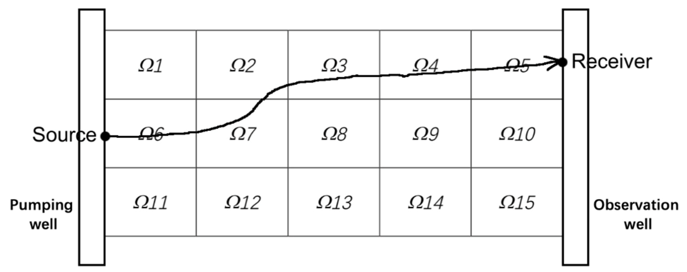
2.1. Hydraulic Travel Time Inversion

The main methodology for travel-time based inversion is based on the findings by Vasco and Datta-Gupta and Brauchler et al. [14,25]. Through their work a relationship between the travel time of a hydraulic signal and the diffusivity within the investigated domain can be established as Equation (1):
t p e a k = 1 c x 1 x 2 d s D ( s ) ,
where t p e a k is the travel time of the pressure signal from the source x 1 to the receiver x 2 ; s is the propagation path of the signal; D ( s ) is the diffusivity along the path; and c is a dimension dependent coefficient. For a two-dimensional (2D) situation it is c = 4; for three-dimensional (3D) it is c = 6.
Figure 1 shows the area Ω between the pumping well and observation well. The area is divided into 15 cells, each denominated discretely as Ω j , where j = 1, …, 15. D j represents the average value of hydraulic diffusivity within the jth cell.
Equation (1) can be rewritten in discrete form, as [40]:
c t i = j = 1 J 1 D j s i j ,     i = 1 ,   ,   I ,     j = 1 ,   ,   J ,
where I is the total number of signals, J is the total number of the cells within the investigation are, anc s i j is the path length of the ith signal through the jth cell.
Equation (2) is reformulated into a matrix form as:
T = S B
T = c t i ,     S = s i j ,     B = 1 D j ,     i = 1 ,   ,   I ,   j = 1 ,   ,   J .

2.2. SIRT Algorithm

Simultaneous iterative reconstruction technique (SIRT) is applied for solving Equation (3) to invert hydraulic diffusion coefficients (D) based on travel time data [40,41].
After setting the current B j e s t equal to the initial value B j i n i t for j = 1, …, J, the following are the steps of SIRT to update the B j e s t value.
Step 1: Perform calculation with Equation (3), providing a predicted T i p r e :
T i p r e = j = 1 J S i j B j e s t ,     i = 1 ,   ,   I .
Step 2: Find the correction for each cell by examining the signals passing through that cell and averaging the corrections suggested by each signal. This operation for the jth cell is defined by:
  Δ B j = 1 W j i = 1 I Δ i B j = 1 W j i = 1 I S i j T i o b s j = 1 J S i j B j e s t j = 1 J S i j 2 ,     j = 1 ,   ,   J .
The weight W j is the number of signals intersecting the jth cell in order to obtain an average correction Δ B j .
Step 3: Determine the new B j ( n e w ) e s t with the average correction Δ B j :
B j ( n e w ) e s t = B j e s t + Δ B j ,       j = 1 , , J .
Then go back to Step 1 and compare the predicted T i p r e with the observed value T o b s . If the difference is larger than the tolerance, go to Step 2 in order to determine a new B j e s t . If the difference is smaller than the defined tolerance, provide the current B j e s t as output.
Based on this algorithm, the derived travel times from pumping tests can be inverted using our self-developed code [41].

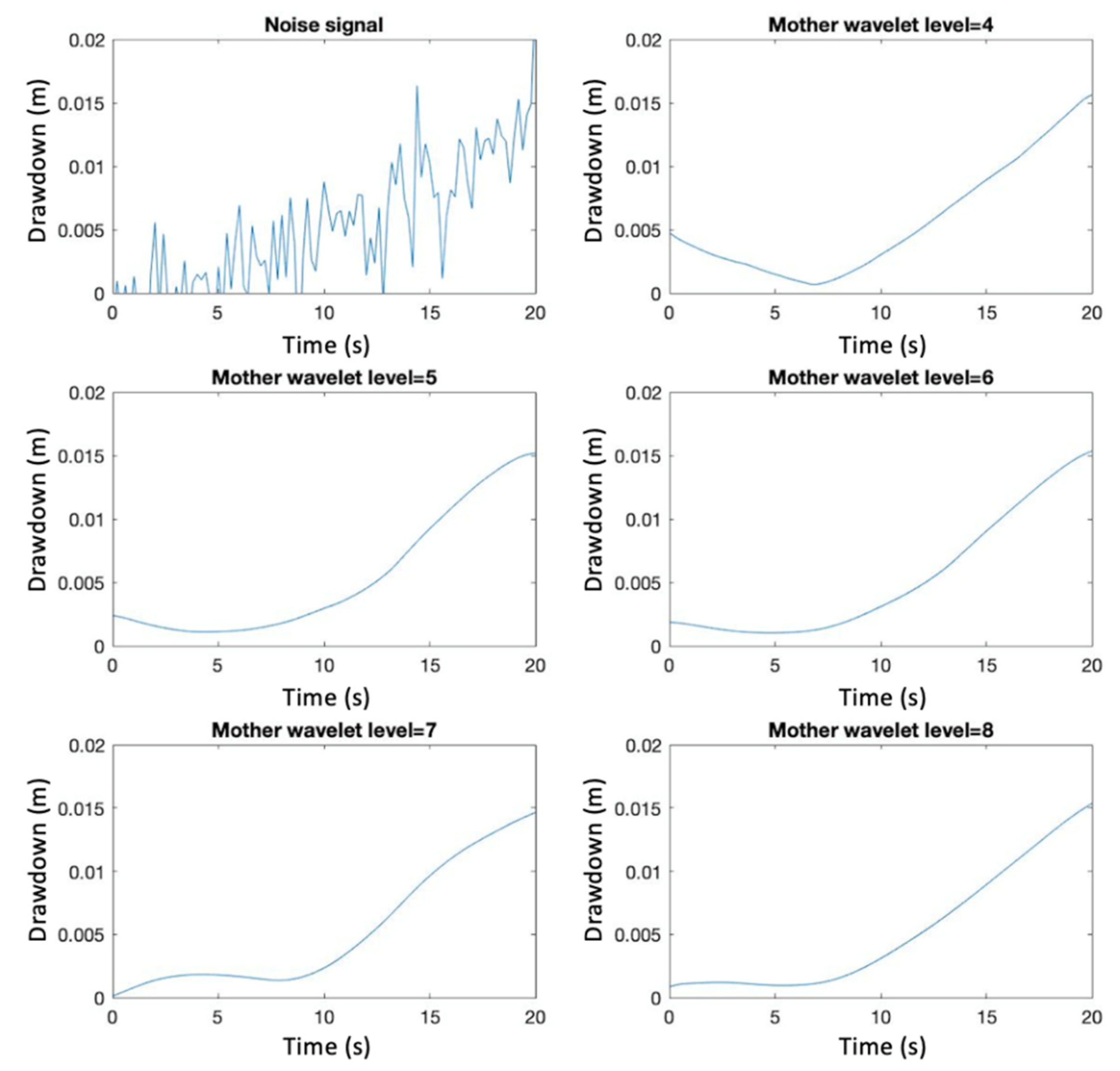
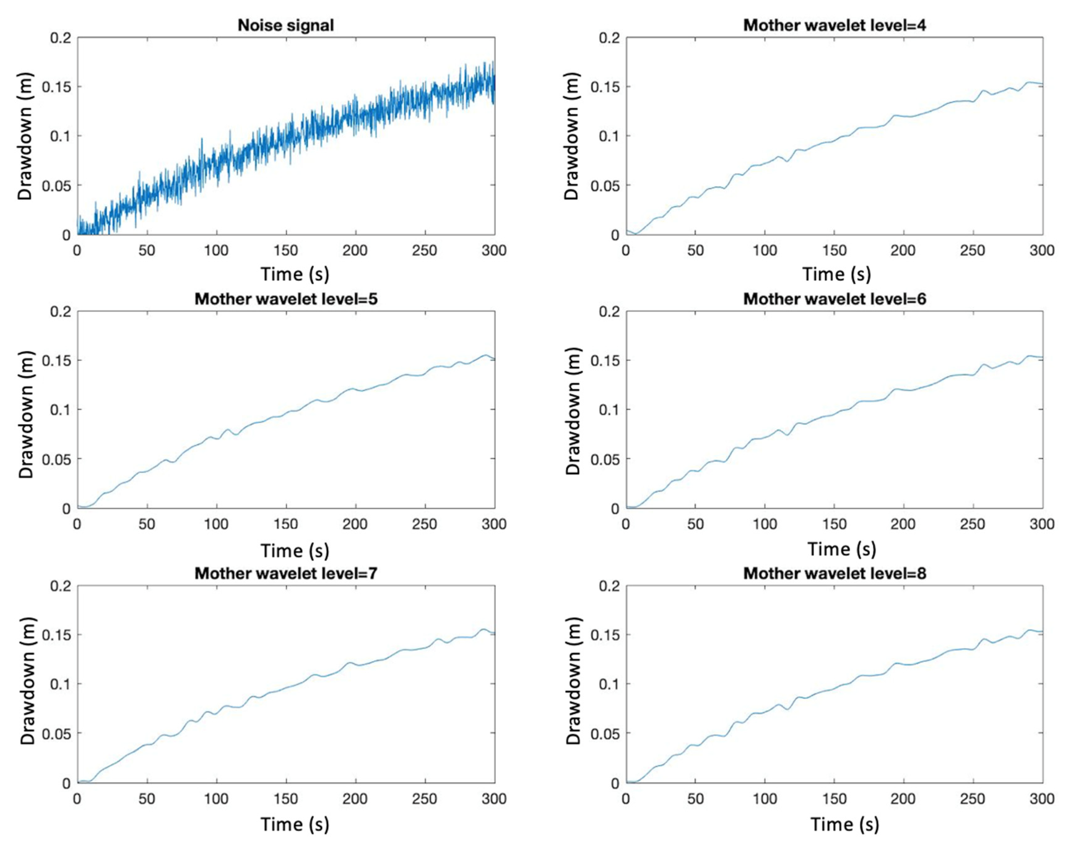
2.3. Wavelet De-Noising

A wavelet is a mathematical function used to separate a given function or continuous-time signal into different scale components [42,43]. Usually one can assign a frequency range to each scale component. Each scale component can then be studied with a resolution that matches its scale. A continuous wavelet transform (CWT) is the representation of a function by wavelets as Equation (7) [43]:
W f ( a , b ) = f , φ a , b ( t ) = 1 a   f ( t ) φ ¯ ( t b a ) d t ,
where f ( t ) is the original signal; a is the scaling factor; b represents the time shift factor; and φ a , b is a finite-length or fast-decaying oscillating waveform, which is known as “mother wavelet”.
Discrete wavelet transform (DWT) is an implementation of the wavelet transform using mutually orthogonal sets of wavelets defined by carefully chosen scaling and shift factors. It leads to an efficient iterative scheme for the transformation. Mallat [34] proposed a wavelet decomposition and reconstruction algorithm, which is known as a two-channel sub-band coder using quadrature mirror filters (QMFs) [44,45]. For an N-sample noised signal a0, the Mallat decomposition algorithm uses orthogonal filters of length L, and can be described as follows:
a j ( i ) = m = 0 L 1 a j 1 ( 2 i m ) h ( m ) , d j ( i ) = m = 0 L 1 a j 1 ( 2 i m ) g ( m ) , 0 i N j 1 ,   1 j log N ,
where a j ( i ) , d j ( i ) are the ith approximation and detail coefficient at level j, respectively. h ( ) , g ( ) are low pass and high pass L-tap filters obtained from the chosen wavelet, respectively. N j = N 2 j is the number of wavelet coefficients in level j.
The Mallat reconstruction algorithm is [45]:
a j ( i ) = n = i / 2 ( L 1 + i ) / 2 a j + 1 ( n ) h ( 2 n i ) + n = i / 2 ( L 1 + i ) / 2 d j + 1 ( n ) g ( 2 n i ) 0 j log N 1 ; 0 i N j 1 .
Wavelet transforming and de-noising, following the Mallat algorithm, were applied in this study using the MATLAB® wavelet analyzer app (Wavelet Toolbox Guide, Mathworks Inc.). The steps of the wavelet de-noising algorithm are given in Figure 2.
In order to remove the noise in a given target signal, Equation (8) is applied to decompose this signal into groups of coefficients at different frequency levels. Based on the different features of the target signal and noise in different frequency segments, certain threshold values are determined and applied to eliminate the noise. Thresholding can be applied by two different methods: hard and soft thresholding. In hard thresholding, elements are set to zero when their absolute values are lower than the threshold value and unchanged when higher than the threshold value. In soft thresholding, the coefficients that exceed the threshold value are softened and decreased by the threshold value. In this study we applied the soft thresholding method since soft thresholding provides smoother de-noising results, which meets the data requirement of hydraulic travel time inversion. After thresholding, the filtered coefficient sets are recomposed to obtain the de-noised signal based on Equation (9).

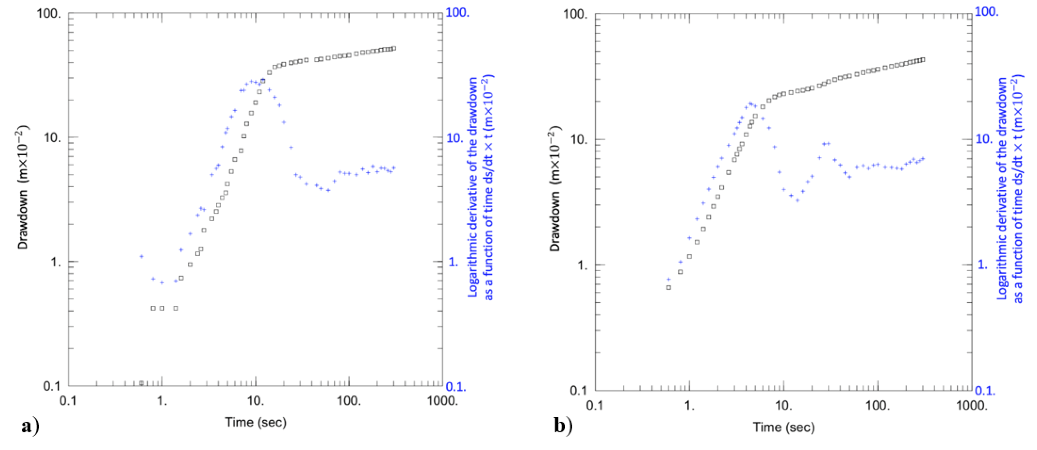
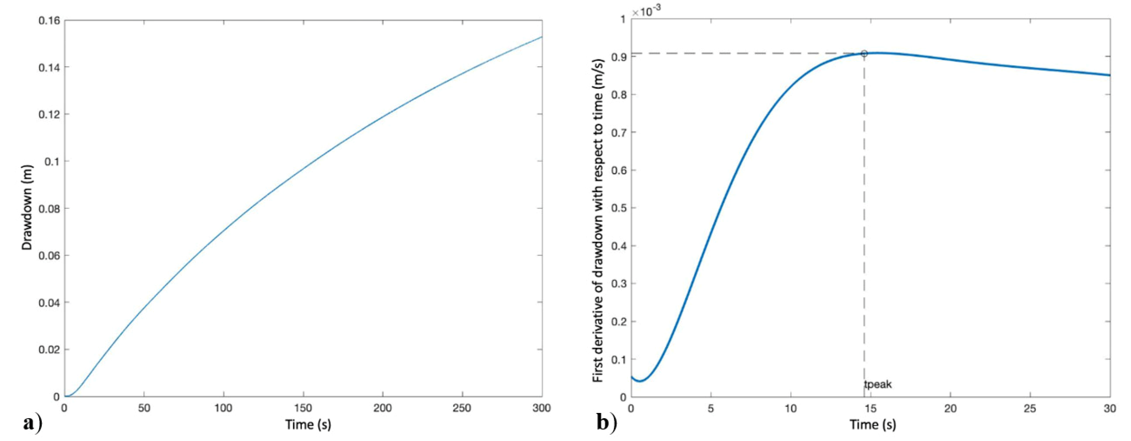
2.4. Diagnostic Plot Analysis

A diagnostic plot is a simultaneous plot of the pumping test induced groundwater level drawdown and the logarithmic derivative of the drawdown as a function of time in a log-log scale [39]. The mathematic expression of the logarithmic derivative of the drawdown as a function of time is shown as Equation (10):
s ln t = t s t ,
where s is the drawdown in the test well and t is the elapsed time since start of pumping.
The logarithmic derivative is highly sensitive to subtle variation in the shape of the drawdown curve and it allows for the detection of aquifer characteristics that are difficult to observe based on the drawdown curve alone. Therefore, the diagnostic plot (the joint use of the drawdown curve and its logarithmic derivative) is applied to characterize the aquifer and flow pattern geometry [46,47]. At the beginning of the plot, a unit slope indicates wellbore storage theoretically. A constant derivative at the immediate time represents a confined homogenous aquifer, while a U-shaped profile during intermediate times might represent an unconfined aquifer or a double porosity aquifer. A decreasing derivative in the late time plot implies a recharge boundary or a 3D flow geometry [46,47], while an increasing derivative indicates a no-flow boundary condition [39].

3. Field Work

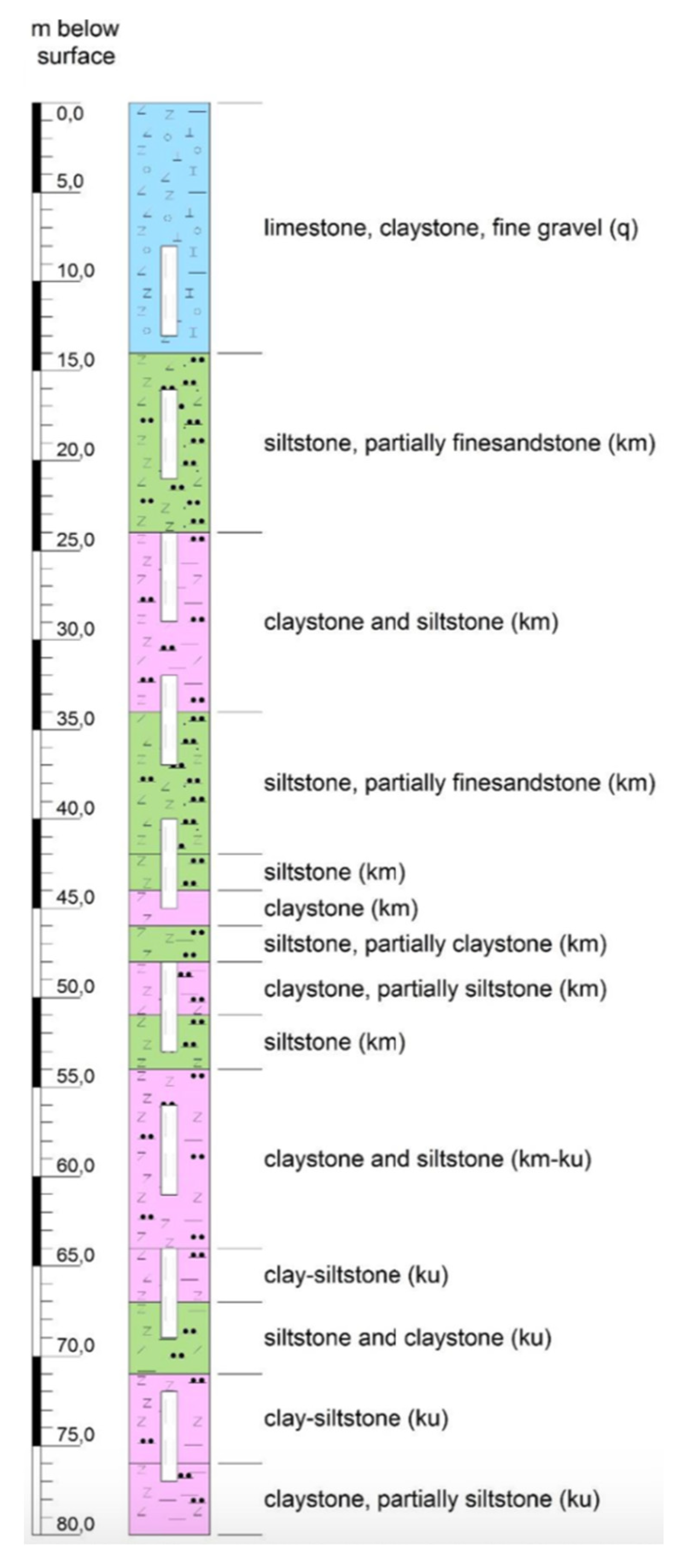
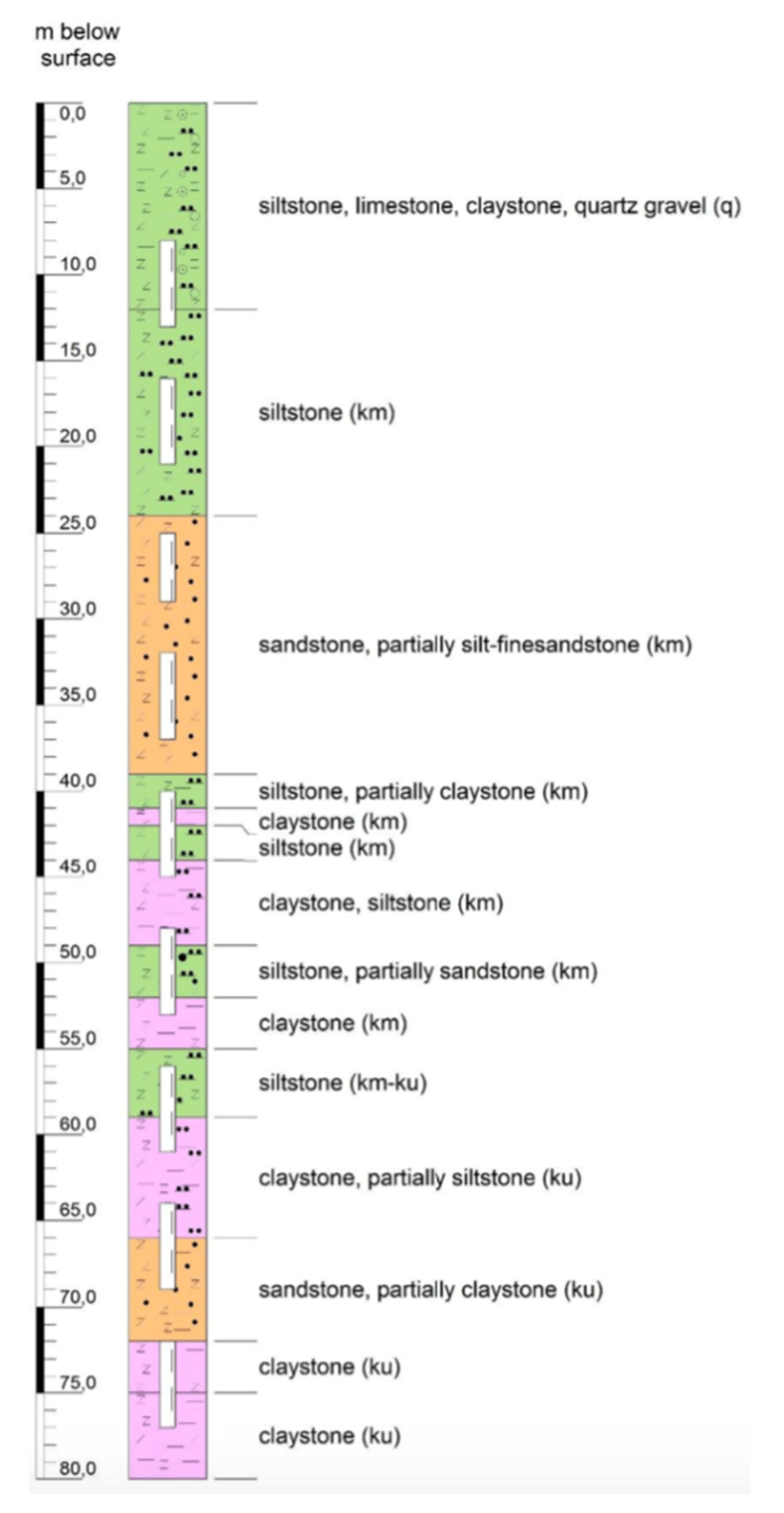
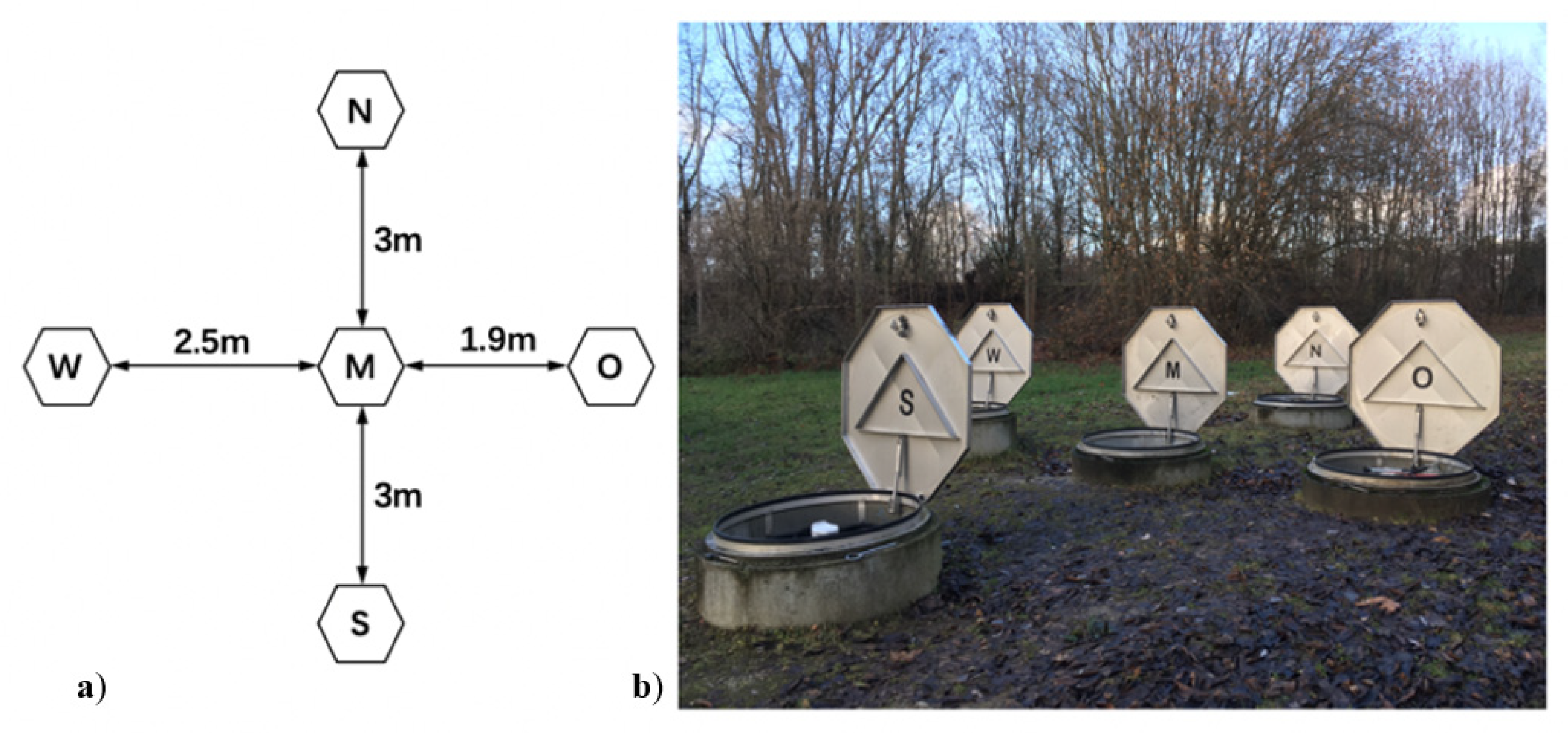
3.1. Test Site Description

The test site is located in the north of Goettingen, Germany. It is at the eastern shoulder of the Leinetalgraben, where a number of folds, faults, and fractures are produced due to polyphase tectonic development under various tension forces and pronounced tectonics in the stories [48]. The test site comprises five 3” (ID 7.62 cm) PVC (Polyvinyl Chloride) wells that are arranged in a cross-shape configuration. The five wells are labeled N, S, W, O, and M for north, south, west, east, and middle, respectively, which represent the cardinal directions of the five wells. Each well is approximately 78 m deep and all five are constructed in the same way, with nine fully cased sections of 3 m length and nine screened sections of 5 m length in alternating order [49]. The screened sections are separated by clay seals within the well gravel pack to allow multilevel measurements. The well network is shown in Figure 3. The main rock types within the research area are limestone, siltstone, and claystone. Detailed well profiles for well O and well M are shown in Appendix A [50].

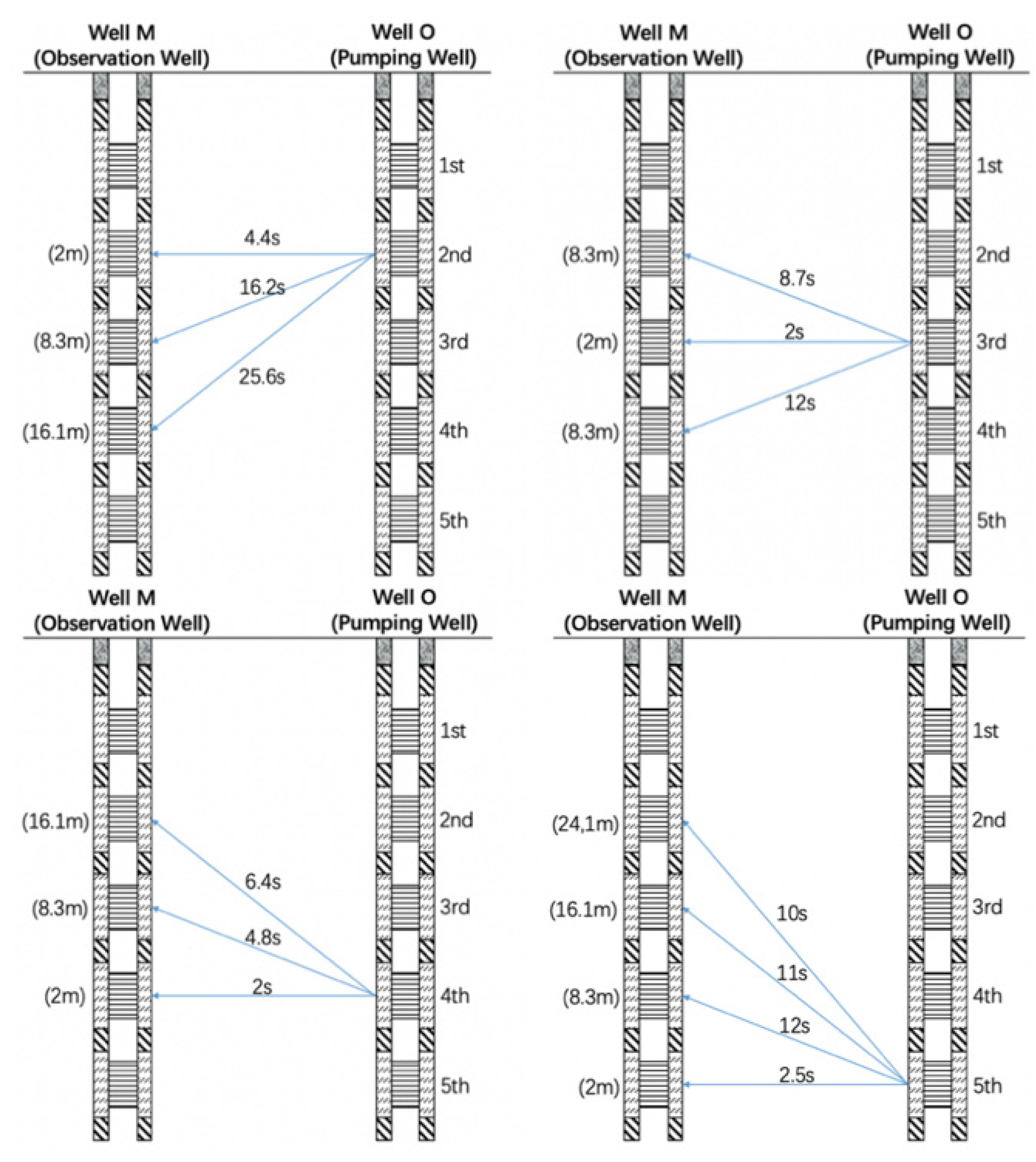
3.2. Multi-Level Pumping Tests Design

A series of multi-level pumping tests were conducted at the test site in April 2018. Figure 4 illustrates the experimental setup. The pumping tests followed a cross-well pattern, which means one well served as pumping (source) well and another well served as an observation (receiver) well. Groundwater was pumped out of well O using a submersible pump (Grundfos MP1, Bjerringbro, Denmark). This pump was connected to a frequency inverter in order to adjust the pumping rate. Pressure transducers were installed in both the pumping well (well O) and the observation well (well M) to monitor the drawdown response during the pumping tests. The drawdown data were recorded by a datalogger Campbell Scientific Micrologger CR3000 (Campbell Scientific, Logan, USA), which was connected to the pressure transducers. Double packer systems were used in both wells to allow depth specific pumping and drawdown measurements. Pressurized air was pumped into the packers to locate the pumping and measuring equipment at a specific depth and to prevent vertical flow within the well.
The double packer systems used in the pumping and observation wells are illustrated in Figure 5.
Following a tomographic configuration, the multi-level pumping tests were conducted in a sequential manner by positioning the pump packer system at a certain well screen and observing subsequently at multiple levels within the observation well. The pump did not work at shallow depth (i.e., at the first screen of the pumping well O) because of the relatively low hydraulic conductivity. Therefore, the pumping tests were conducted starting from the second screen to the fifth well screen. The second to the fifth screens of pumping well O were acting as source points, while the second to the fifth screens of observation well M were acting as receiving points in the tests (compare Figure 1). Given a 4 by 4 distribution in the sequential cross-hole configuration, 16 source-receiver pairs of data, with which 16 travel time data can be calculated, were obtained during the multi-level pumping tests. Figure 6 depicts the multi-level cross-hole array between the well O and the well M. The straight lines in the figure are not the real hydraulic signal travel paths. They demonstrate the spatial configuration of the source and receiver locations.

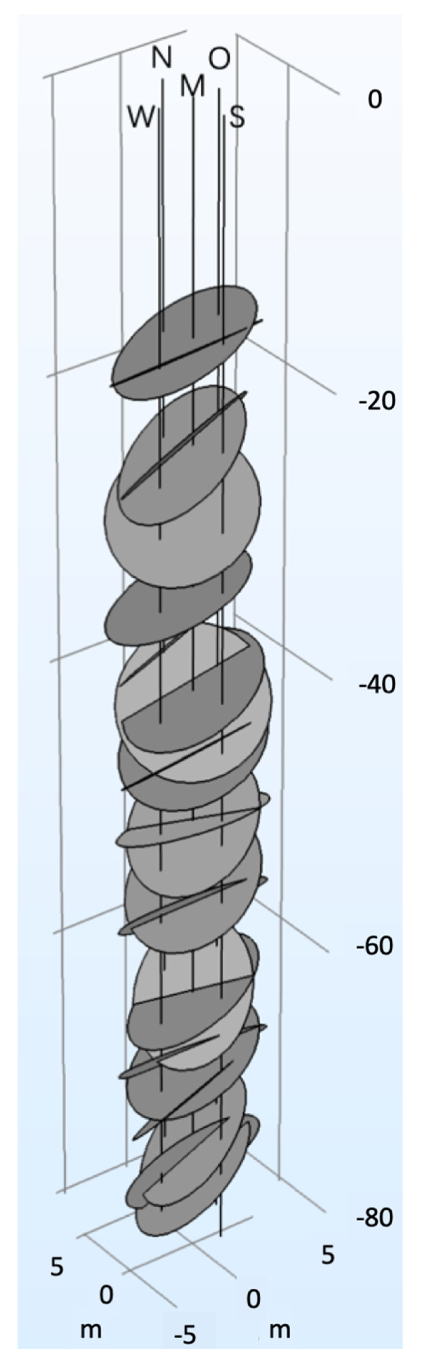
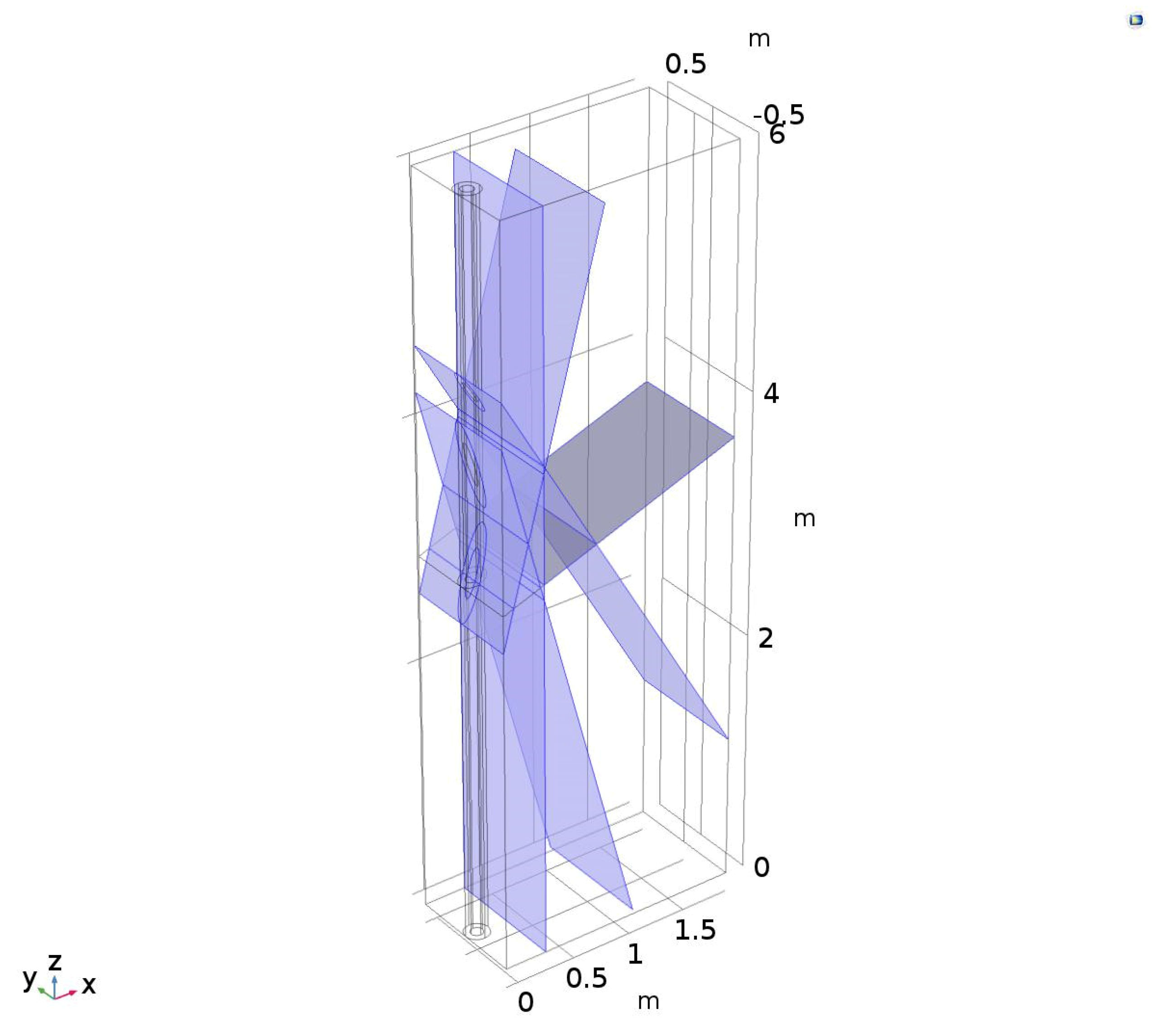
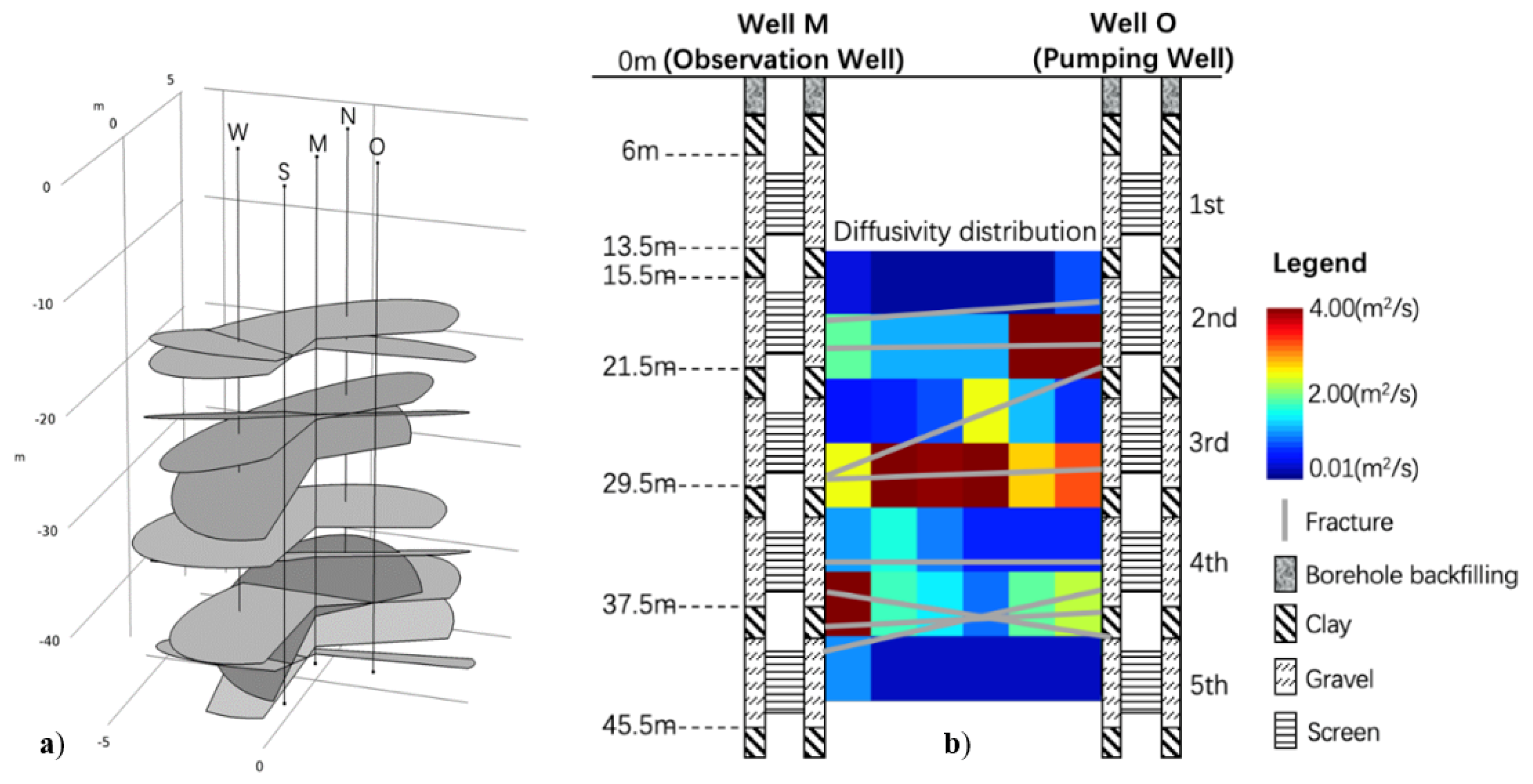
3.3. D Fracture Geometry Model

A 3D aquifer fracture geometry model of this test site was set up by Werner [51]. This model is based on geophysical data, distribution of calcite veins, paleostress field analysis, and microthermometry. Figure 7 shows an example of the rock samples which were obtained at the test site during the drilling process. With these data the possible positions and distributions of the fractures in the aquifer can be digitalized and visualized. Based on the result of Werner’s study, we set up a 3D fracture geometry model using the COMSOL® Multiphysics software (COMSOL, Inc., Burlington, USA). An illustration of the 3D fracture geometry model is shown in Appendix B.
The inversion result obtained within our study will be compared with this 3D fracture geometry model.

4. Numerical Study

4.1. Numerical Modelling

A 3D numerical groundwater model, based on field data from the test site, was built to simulate the pumping tests performed in well O using the COMSOL® Multiphysics software with the physics module “Darcy’s law”. The size of the investigated subsurface zone was set to 1.9 m × 1 m × 6 m, where 6 m is the length of one screen in the well O and 1.9 m is the distance between well O and well M. A mass flux point was set in the pumping well to simulate the pumping process and an observation point was set at the horizontally corresponding position of the observation well (1.9 m away from the pumping well). The mass flux was set to 10.2 L/min, according to the average pumping rate in the field experiments. Infinite element domains were established in all directions outside the investigated zone in order to eliminate boundary effects. An illustration of the numerical model setup is shown in Figure 8. The one-screen investigation zone model is a simplification of a multi-level pumping test at the test site, of which the depth orientated pumping and the water head measurement are at the same depth, with the assumption that the double-packer systems can totally prevent vertical flow within both pumping and observation wells. Thus, the remaining part of the well does not contribute to the pumping test. The aim of this modelling is to find the optimal de-noising parameters. The 3D-effects on the head response due to the other screens are not considered in this simulation.
The initial setting of the hydraulic parameters in the model was based on the former investigation work at the test site [52,53]. In order to ensure that the numerical model provides a similar hydraulic behavior compared to the real test site, the hydraulic parameters of the model were calibrated to match the drawdown and the calculated diagnostic plot to the observed data and diagnostic plot from the field experiment (Figure 9). The final setting of the model parameters is shown in Table 1. The diagnostic plots of one set of real experimental drawdown data from pumping well O (Figure 9a) and the simulated data from the numerical model (Figure 9b) are shown below. The black curve is the drawdown curve while the blue curve shows its derivative with respect to time.
As shown in Figure 9, the logarithmic derivatives in both plots increase rapidly with a slope of approximately 1 from 1 s to 8 s, which indicates the presence of borehole storage effects. The U-shaped profiles of both derivative curves after 10 s represents double-porosity properties, which is consistent with the porous-fractured aquifer character of the test site. In general, the diagnostic plot of the numerically simulated drawdown data shows the same pattern as that from the field data, which indicates that the model aquifer has similar properties as the real one. Thus, the simulated data from the numerical model can be used to find a suitable method to de-noise the field experimental data.
In the model, an observation point corresponding to the position of well M was also set, which is 1.9 m away from the pumping well O. The simulated drawdown response at the observation point is shown in Figure 10a. Figure 10b shows the first derivative of the drawdown with respect to time. As shown in Figure 10b, the time tpeak at the derivative maximum, a measure for the hydraulic signal travel time, is 14.6 s.

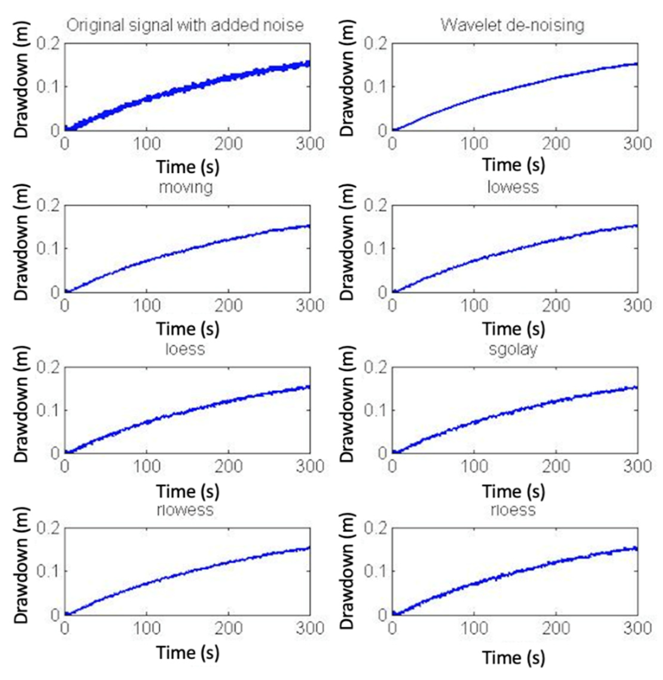
4.2. Comparison Between Wavelet and Other Filters

Gaussian white noise was added to the numerically simulated drawdown curves in order to compare the results of the wavelet de-noising method with six filters provided with the MATLAB® (The MathWorks, Inc., Natick, USA) “smooth” command (the names of those filters are moving, lowess, loess, sgolay, rlowess and rloess).
Wavelet de-noising was performed with the integrated “Wavelet Analyzer” of MATLAB®. Mother wavelet “Symlets” was selected and the mother wavelet level was set to eight. The de-noising level was set to five. Figure 11 shows the original signal with a 30 signal-to-noise ratio Gaussian white noise, the de-noising result of wavelet de-noising, and the de-noising results of the six different filters.
The travel time value tpeak of each de-noised signal was calculated. The calculation results are shown in Table 2.
As shown in the table, the tpeak value derived from the result of wavelet de-noising is the closest to the known “true” tpeak value, which is 14.6 s (Section 4.1). The difference among the results of the seven de-noising methods is not significant. However, since the tpeak value in real experiments can be very small, small differences can cause large deviations of final results. Therefore, although the lead is not prominent, we conclude that the wavelet de-noising method has the best de-noising performance and that it is suitable to be utilized to de-noise the experimental data obtained from the pumping tests.

4.3. Wavelet De-Noising Method

So far, it is shown that the wavelet de-noising method is suitable to de-noise the experimental drawdown data obtained from the pumping tests. However, which mother wavelet and which de-noising level should be selected to remove the noise in the experimental drawdown signal and to get the most accurate travel time value is not yet known. The simulated drawdown response and the already known time tpeak from the numerical model were used to find the best wavelet de-noising method to de-noise the experimental data. Three variables were investigated: wavelet type, mother wavelet level, and de-noising level.
Since the experimental conditions may change from day to day, the noise levels in the drawdown data can be different. Therefore, Gaussian white noise with different signal-to-noise ratios (10, 20, 30, and 40) was added to the simulated drawdown response from the numerical model.
Different mother wavelet types were tested in this study and four different types of mother wavelets were found effective for our work. The names of these four mother wavelets are “Symlets”, “Coiflets”, “Biorthogonal”, and “Dmey” (Wavelet Toolbox Guide, The MathWorks Inc., Natick, USA).
The level of the mother wavelet is a parameter of the de-noising method. In order to find the influence of the mother wavelet level on the de-noising result, the simulated drawdown curve with a signal-to-noise ratio of 20 noise was selected as the de-noising object, “Symlets” was selected as the mother wavelet, and the de-noising level was set to five, the mother wavelet level was varied from four to eight to de-noise the signal (level eight is the optional maximum level in MATLAB® wavelet app), and the de-noising results are shown in Figure 12.
As shown in Figure 12, there is not a particularly big difference in the de-noising results with different mother wavelet levels. Therefore, the mother wavelet level is not a sensitive parameter in this study. It also holds if the de-noising level is changed. However, if we zoom into the figure and focus on the beginning part of the curve (Figure 13), which is the most important part for travel time derivation, it is found in the figure that the higher the mother wavelet level, the smoother the signal curve after de-noising. Since the drawdown curve should be a smooth curve, and the first derivative is required for seeking the travel time, the level of the mother wavelet level was selected to the highest level in the following study.
The type of the mother wavelet and the de-noising level are the two other parameters in the de-noising method. Therefore, the drawdown data with different noise levels (signal-noise-ratio (SNR) = 40, 30, 20, 10) were de-noised with four different mother wavelets, and with different de-noising levels (level = 5, 6, and 7) respectively. The de-noising results were then used to calculate the travel time tpeak using MATLAB®. The de-noising results with lower de-noising levels (i.e., lower than level 4) were not smooth enough and can hardly be used for further calculation of the tpeak.
The results are summarized in Table 3. Based on the numerical model simulation, the exact travel time tpeak should be 14.6 s (Section 4.1).
The slash in the table means that no unique tpeak can be found from the first derivative curve, because of the high level of noise and poor de-noising result.
After analyzing the results in Table 3, several conclusions can be drawn:
In general, the results using mother wavelets “Coiflets” and “Dmey” are relatively better than the ones using “Symlets” and “Biorthogonal”.
Mother wavelet “Dmey” is suitable for de-noising less noisy signals with low de-noising levels (level five particularly).
Mother wavelet “Coiflets” behaves the best when the noise is relatively large and the de-noising level is six.
When the de-noising level is seven, the relative error of the derived travel time tpeak is relatively large, i.e., the derived travel time value is not accurate.
When the signal-to-noise ratio is smaller than 20, wavelet de-noising cannot effectively remove noise signals. Therefore, the travel time value calculated from the de-noising result is not reliable.
Although the noise is added artificially and the noise is merely Gaussian white noise, the wavelet de-nosing method used in this study is not capable to completely remove the noise and to get the exact ‘true’ travel time value.
In the actual field drawdown data, the noise is generally large and the signal-to-noise ratio is usually between 20 and 30. It can be found from Table 3 that whether the signal-to-noise ratio is 20 or 30, the travel times derived using “Coiflets” mother wavelet and de-noising level six are closest to the ‘true’ travel time value. Therefore, mother wavelet “Coiflets”, with mother wavelet level five and de-noising level 6 are used in this study to process the field data.

5. Results

5.1. Travel Time Results from Experimental Data

Using the wavelet de-noising parameters defined above, the field data from multi-level pumping tests were processed to remove the noise signal, and the de-noising results were used to obtain the travel time values tpeak. Figure 14 shows an example of data processing of a field data set. The tpeak results of all pumping tests are summarized in Figure 15. The figure also shows the calculated distance between the pumping source and the observation point based on the well construction profiles and well arrangement (in bracket). The travel time results for O2M5 (the second screen of well O as a source and the fifth screen of well M as a receiver), O3M5 (the third screen of well O as a source and the fifth screen of well M as a receiver), and O4M5 (the fourth screen of well O as a source and the fifth screen of well M as a receiver) are missing, because the noise of these field data sets is too high to obtain reliable travel time values.
As shown in Figure 15, since the distance between the signal source and receiver location is relatively small, the signal travel time for horizontal directions (e.g., O2M2) is relatively short. The signal travel time for experiments with a high slope between the signal source and the receiver locations (e.g., O2M4) is relatively large because of the longer travel distance. However, the difference in travel time can be observed in the case of a similar distance between the source and receiver. For instance, the travel time from the fourth screen of well O to the second screen of M (6.4 s) is significantly smaller than the travel time from the second screen of well O to the fourth screen of M (25.6 s), while the travel distances within the two experiments are basically identical. The explanation is that the hydraulic connection between the fourth screen of well O and the second screen of M is better compared with the other setup, due to a possibly existing fracture.

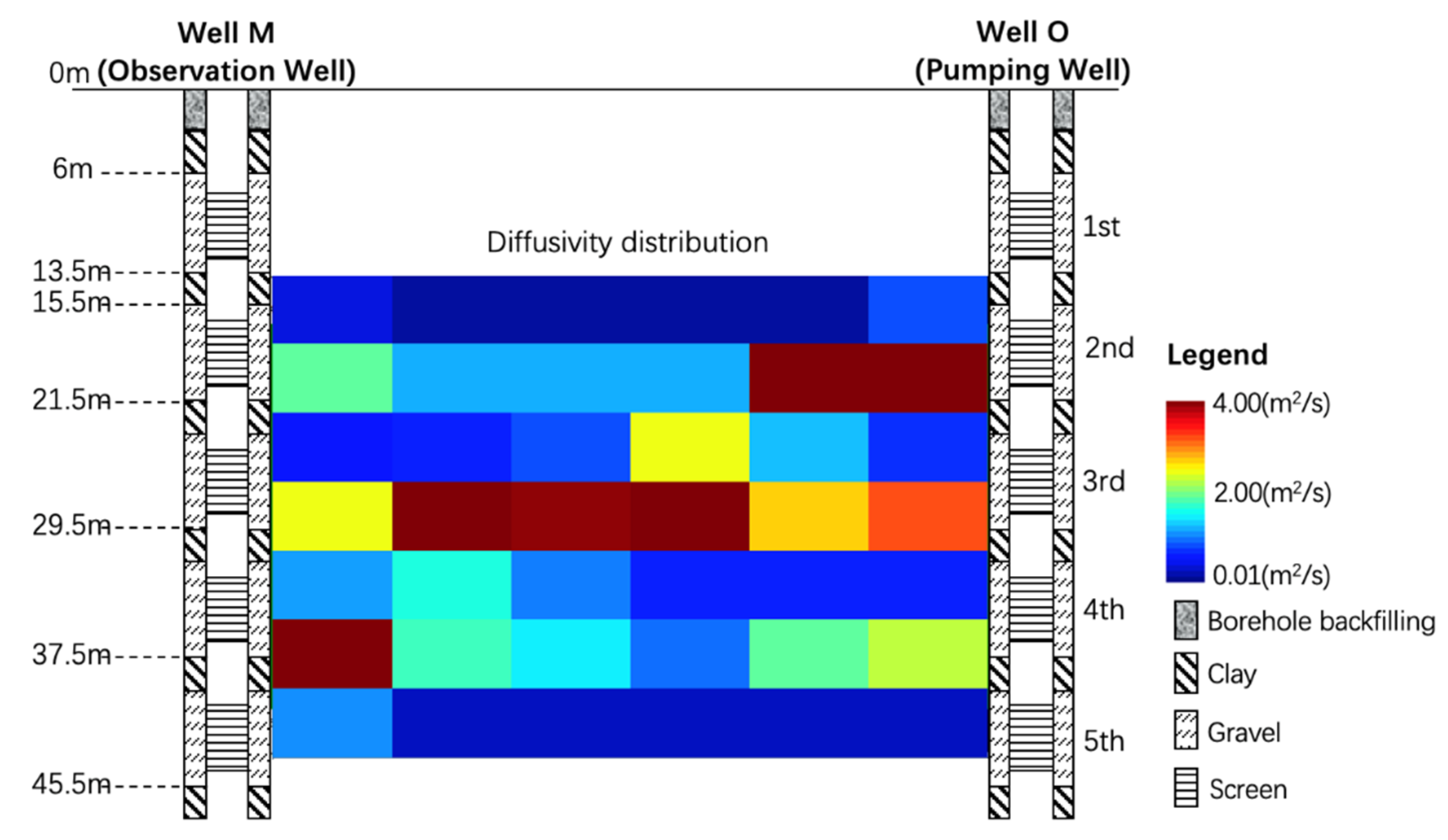
5.2. Hydraulic Travel Time Inversion Result and 3D Fracture Geometry Model

The diffusivity distribution based on inversion using the SIRT algorithm is shown in Figure 16. The main features of the inversion result are the three-horizontal high-diffusivity channels between well O and well M. The diffusivity of the cross section is relatively high near each well screen.
Figure 17a shows the result of a geological 3D fracture geometry model of the top 45 m based on the data introduced in Section 3.3 and Figure 17b shows the 2D travel-time based inversion result for comparison purposes.
The grey lines in Figure 17b are possible locations of fractures based on the 3D geometry model. In general, the zones where a fracture may exist according to the 3D geometry model have higher diffusivity values in the inversion result. Although there are slight deviations, the generally consistent fracture locations and high diffusivity zones indicate a reliable diffusivity distribution within the study area obtained from the travel-time based hydraulic tomography.

6. Conclusions

In this study, travel-time based hydraulic tomography was used to identify the two-dimensional hydraulic diffusivity distribution between a pumping and a drawdown observation well at our test site. The agreement between the obtained hydraulic diffusivity distribution and the geological 3D geometry model proves the reliability of the hydraulic tomography result. The employed travel-time based inversion requires accurate hydraulic signal travel time values, which determine the quality of the inversion result.
The major obstacle in getting accurate travel times is the noise in the experimental drawdown curves. In order to find the best way to de-noise the drawdown curves, a numerical 3D model based on our test site data was established in this study. Using diagnostic plots, it was demonstrated that the model provides a hydrogeological behavior according to the test site situation. By using wavelet and other filters to de-noise numerically simulated pumping test drawdown curves, with added Gaussian white noise, the wavelet de-noising method, with mother wavelet “Coiflets”, mother wavelet level five, and de-noising level six, proved to have the best performance in processing the noisy data.
Although the best de-noising method was found in this study, it cannot totally remove the noise, which might still influence the accuracy of the result. In addition, this study assumes that the noise in the experimental data was white noise. If the experimental data contain other types of noise, the de-noising method introduced in this study should be further tested and if needed improved.

Author Contributions

H.Y. performed the data processing and numerical modeling, participated in the field experiment and wrote the manuscript. R.H. supervised the field work and manuscript writing. P.Q. performed inversion work, provided modifications to the manuscript and participated in the field experiment. Q.L. organized the field experiment, supervised the numerical modeling. Y.X. and R.T. took part in the experiment and provided necessary suggestions. T.P. supervised the whole work and provided necessary solutions for various problems. All authors have read and agreed to the published version of the manuscript.

Funding

This publication was funded by the Open Access Publication Funds of the Goettingen University.

Conflicts of Interest

The authors declare no conflict of interest.

Appendix A

Figure A1. Well profile for well O [50].
Water 12 01533 g0a1
Figure A2. Well profile for well M [50].
Water 12 01533 g0a2

Appendix B

Figure A3. Illustration of the 3D fracture model (gray planes depict the possible positions of fractures) [51].
Water 12 01533 g0a3

References

  1. Illman, W.A.; Craig, A.J.; Liu, X. Practical issues in imaging hydraulic conductivity through hydraulic tomography. Ground Water 2008, 46, 120–132. [Google Scholar] [CrossRef] [PubMed]
  2. Illman, W.A.; Liu, X.; Takeuchi, S.; Yeh, T.C.J.; Ando, K.; Saegusa, H. Hydraulic tomography in fractured granite: Mizunami Underground Research site, Japan. Water Resour. Res. 2009, 45, W01406. [Google Scholar] [CrossRef] [Green Version]
  3. Illman, W.A. Hydraulic tomography offers improved imaging of heterogeneity in fractured rocks. Groundwater 2014, 52, 659–684. [Google Scholar] [CrossRef]
  4. Illman, W.A. Lessons learned from hydraulic and pneumatic tomography in fractured rocks. Procedia Environ. Sci. 2015, 25, 127–134. [Google Scholar] [CrossRef] [Green Version]
  5. Yeh, T.C.J.; Liu, S.Y. Hydraulic tomography: Development of a new aquifer test method. Water Resour. Res. 2000, 36, 2095–2105. [Google Scholar] [CrossRef]
  6. Yeh, T.C.; Mao, D.; Zha, Y.; Hsu, K.C.; Lee, C.H.; Wen, J.C.; Lu, W.; Yang, J. Why hydraulic tomography works? Ground Water 2014, 52, 168–172. [Google Scholar] [CrossRef]
  7. Sun, R.L.; Yeh, T.C.J.; Mao, D.Q.; Jin, M.G.; Lu, W.X.; Hao, Y.H. A temporal sampling strategy for hydraulic tomography analysis. Water Resour. Res. 2013, 49, 3881–3896. [Google Scholar] [CrossRef]
  8. Sanchez-Leon, E.; Leven, C.; Haslauer, C.P.; Cirpka, O.A. Combining 3D Hydraulic Tomography with Tracer Tests for Improved Transport Characterization. Ground Water 2016, 54, 498–507. [Google Scholar] [CrossRef]
  9. Zha, Y.; Yeh, T.C.J.; Illman, W.A.; Zeng, W.; Zhang, Y.; Sun, F.; Shi, L. A reduced-order successive linear estimator for geostatistical inversion and its application in hydraulic tomography. Water Resour. Res. 2018, 54, 1616–1632. [Google Scholar] [CrossRef]
  10. Zha, Y.; Yeh, T.-C.J.; Illman, W.A.; Tanaka, T.; Bruines, P.; Onoe, H.; Saegusa, H. What does hydraulic tomography tell us about fractured geological media? A field study and synthetic experiments. J. Hydrol. 2015, 531, 17–30. [Google Scholar] [CrossRef]
  11. Zhu, J.F.; Yeh, T.C.J. Characterization of aquifer heterogeneity using transient hydraulic tomography. Water Resour. Res. 2005, 41, W07028. [Google Scholar] [CrossRef]
  12. Liu, X.; Illman, W.A.; Craig, A.J.; Zhu, J.; Yeh, T.C. Laboratory sandbox validation of transient hydraulic tomography. Water Resour. Res. 2007, 43, W05404. [Google Scholar] [CrossRef]
  13. Brauchler, R.; Sauter, M.; McDermott, C.I.; Leven, C.; Weede, M.; Dietrich, P.; Liedl, R.; Hötzl, H.; Teutsch, G. Characterization of fractured porous media: Aquifer analogue approach. Groundw. Fract. Rocks Iah Sel. Pap. Ser. 2007, 9, 375. [Google Scholar]
  14. Brauchler, R.; Hu, R.; Dietrich, P.; Sauter, M. A field assessment of high-resolution aquifer characterization based on hydraulic travel time and hydraulic attenuation tomography. Water Resour. Res. 2011, 47, W03503. [Google Scholar] [CrossRef]
  15. Hao, Y.; Yeh, T.-C.J.; Xiang, J.; Illman, W.A.; Ando, K.; Hsu, K.-C.; Lee, C.-H. Hydraulic tomography for detecting fracture zone connectivity. Groundwater 2008, 46, 183–192. [Google Scholar] [CrossRef]
  16. Hu, R.; Brauchler, R.; Herold, M.; Bayer, P. Hydraulic tomography analog outcrop study: Combining travel time and steady shape inversion. J. Hydrol. 2011, 409, 350–362. [Google Scholar] [CrossRef]
  17. Nolet, G. A breviary of seismic tomography. A Breviary of Seismic Tomography, by Guust Nolet; Cambridge University Press: Cambridge, UK, 2008; Volume 2008. [Google Scholar]
  18. Tarantola, A. Inverse Problem Theory and Methods for Model Parameter Estimation; Siam: Philadelphia, PA, USA, 2005; Volume 89. [Google Scholar]
  19. Wang, Y.L.; Yeh, T.C.J.; Wen, J.C.; Huang, S.Y.; Zha, Y.; Tsai, J.P.; Hao, Y.; Liang, Y. Characterizing subsurface hydraulic heterogeneity of alluvial fan using riverstage fluctuations. J. Hydrol. 2017, 547, 650–663. [Google Scholar] [CrossRef]
  20. Zha, Y.; Yeh, T.J.; Illman, W.A.; Tanaka, T.; Bruines, P.; Onoe, H.; Saegusa, H.; Mao, D.; Takeuchi, S.; Wen, J.C. An Application of Hydraulic Tomography to a Large-Scale Fractured Granite Site, Mizunami, Japan. Ground Water 2016, 54, 793–804. [Google Scholar] [CrossRef]
  21. Brauchler, R.; Hu, R.; Vogt, T.; Al-Halbouni, D.; Heinrichs, T.; Ptak, T.; Sauter, M. Cross-well slug interference tests: An effective characterization method for resolving aquifer heterogeneity. J. Hydrol. 2010, 384, 33–45. [Google Scholar] [CrossRef]
  22. Brauchler, R.; Liedl, R.; Dietrich, P. A travel time based hydraulic tomographic approach. Water Resour. Res. 2003, 39, 1370. [Google Scholar] [CrossRef]
  23. Brauchler, R.; Cheng, J.T.; Dietrich, P.; Everett, M.; Johnson, B.; Liedl, R.; Sauter, M. An inversion strategy for hydraulic tomography: Coupling travel time and amplitude inversion. J. Hydrol. 2007, 345, 184–198. [Google Scholar] [CrossRef]
  24. Cheng, J.T.; Brauchler, R.; Everett, M.E. Comparison of Early and Late Travel Times of Pressure Pulses Induced by Multilevel Slug Tests. Eng. Appl. Comput. Fluid Mech. 2009, 3, 514–529. [Google Scholar] [CrossRef]
  25. Vasco, D.W.; Keers, H.; Karasaki, K. Estimation of reservoir properties using transient pressure data: An asymptotic approach. Water Resour. Res. 2000, 36, 3447–3465. [Google Scholar] [CrossRef]
  26. Ott, H.W.; Ott, H.W. Noise Reduction Techniques in Electronic Systems; Wiley: New York, NY, USA, 1988; Volume 442. [Google Scholar]
  27. Tuzlukov, V. Signal Processing Noise; CRC Press: Boca Raton, FL, USA, 2002. [Google Scholar]
  28. Rouphael, T.J. RF and Digital Signal Processing for Software-Defined Radio: A Multi-standard Multi-mode Approach; Newnes: Oxford, UK, 2009. [Google Scholar]
  29. McClaning, K.; Vito, T. Radio Receiver Design; Noble Publishing Corporation: Atlanta, GA, USA, 2000. [Google Scholar]
  30. Illman, W.A.; Liu, X.; Craig, A. Steady-state hydraulic tomography in a laboratory aquifer with deterministic heterogeneity: Multi-method and multiscale validation of hydraulic conductivity tomograms. J. Hydrol. 2007, 341, 222–234. [Google Scholar] [CrossRef]
  31. Tokhmechi, B.; Memarian, H.; Rasouli, V.; Noubari, H.A.; Moshiri, B. Fracture detection from water saturation log data using a Fourier–wavelet approach. J. Pet. Sci. Eng. 2009, 69, 129–138. [Google Scholar] [CrossRef] [Green Version]
  32. Taherdangkoo, R.; Abdideh, M. Application of wavelet transform to detect fractured zones using conventional well logs data (Case study: Southwest of Iran). Int. J. Pet. Eng. 2016, 2, 125–139. [Google Scholar] [CrossRef]
  33. Xie, H.; Pierce, L.E.; Ulaby, F.T. SAR speckle reduction using wavelet denoising and Markov random field modeling. Ieee Trans. Geosci. Remote Sens. 2002, 40, 2196–2212. [Google Scholar] [CrossRef] [Green Version]
  34. Quiroga, R.Q.; Garcia, H. Single-trial event-related potentials with wavelet denoising. Clin. Neurophysiol. 2003, 114, 376–390. [Google Scholar] [CrossRef]
  35. Xiang, J.; Yeh, T.C.J.; Lee, C.H.; Hsu, K.C.; Wen, J.C. A simultaneous successive linear estimator and a guide for hydraulic tomography analysis. Water Resour. Res. 2009, 45, W02432. [Google Scholar] [CrossRef] [Green Version]
  36. Brauchler, R.; Hu, R.; Hu, L.; Jiménez, S.; Bayer, P.; Dietrich, P.; Ptak, T. Rapid field application of hydraulic tomography for resolving aquifer heterogeneity in unconsolidated sediments. Water Resour. Res. 2013, 49, 2013–2024. [Google Scholar] [CrossRef]
  37. Guo, X.-L.; Yang, K.-L.; Guo, Y.-X. Hydraulic pressure signal denoising using threshold self-learning wavelet algorithm. J. Hydrodyn. Ser. B 2008, 20, 433–439. [Google Scholar] [CrossRef]
  38. Bourdet, D.; Whittle, T.M.; Douglas, A.A.; Pirard, Y.M. A New Set of Type Curves Simplifies Well Test Analysis. World Oil 1983, 196, 95. [Google Scholar]
  39. Renard, P.; Glenz, D.; Mejias, M. Understanding diagnostic plots for well-test interpretation. Hydrogeol. J. 2009, 17, 589–600. [Google Scholar] [CrossRef] [Green Version]
  40. Lo, T.-W.; Inderwiesen, P.L. Fundamentals of Seismic Tomography; Society of Exploration Geophysicists: Houston, TX, USA, 1994; Volume 6. [Google Scholar]
  41. Qiu, P.X.; Hu, R.; Hu, L.W.; Liu, Q.; Xing, Y.X.; Yang, H.C.; Qi, J.J.; Ptak, T. A Numerical Study on Travel Time Based Hydraulic Tomography Using the SIRT Algorithm with Cimmino Iteration. Water 2019, 11, 909. [Google Scholar] [CrossRef] [Green Version]
  42. Addison, P.S. The Illustrated Wavelet Transform Handbook: Introductory Theory and Applications in Science, Engineering, Medicine and Finance; CRC Press: Boca Raton, FL, USA, 2002; Volume 6. [Google Scholar]
  43. Chui, C.K. An Introduction to Wavelets; Elsevier: Amsterdam, The Netherlands, 2016; Volume 6. [Google Scholar]
  44. Shensa, M.J. The Discrete Wavelet Transform-Wedding the a Trous and Mallat Algorithms. IEEE Trans. Signal Process. 1992, 40, 2464–2482. [Google Scholar] [CrossRef] [Green Version]
  45. Mallat, S.G. A Theory for Multiresolution Signal Decomposition—The Wavelet Representation. IEEE Trans. Pattern Anal. Mach. Intell. 1989, 11, 674–693. [Google Scholar] [CrossRef] [Green Version]
  46. Illman, W.A.; Neuman, S.P. Type-curve interpretation of multirate single-hole pneumatic injection tests in unsaturated fractured rock. Groundwater 2000, 38, 899–911. [Google Scholar] [CrossRef]
  47. Illman, W.A.; Neuman, S.P. Type curve interpretation of a cross-hole pneumatic injection test in unsaturated fractured tuff. Water Resour. Res. 2001, 37, 583–603. [Google Scholar] [CrossRef]
  48. Tanner, D.C.; Leiss, B.; Vollbrecht, A. The role of strike-slip tectonics in the Leinetal Graben, Lower Saxony [Die Bedeutung von Seitenverschiebungstektonik im Leinetalgraben, Niedersachsen]. Z. Der Dtsch. Ges. für Geowiss. 2010, 161, 369–377. [Google Scholar]
  49. Oberdorfer, P.; Holzbecher, E.; Hu, R.; Ptak, T.; Sauter, M. A Five Spot Well Cluster for Hydraulic and Thermal Tomography, Proceedings of the Thirty-Eighth Workshop on Geothermal Reservoir Engineering, Stanford, CA, USA, 11–13 February 2013; Stanford Geothermal Program: Stanford, CA, USA, 2013; pp. 239–243. [Google Scholar]
  50. Baetzel, K. Hydrogeological Characterization of a Fratured Aquifer based on Modelling and Heat Tracer Experiments. Master‘s Thesis, University of Goettingen, Goettingen, Lower Saxony, Germany, 2017. [Google Scholar]
  51. Werner, H. Strukturgeologische Charakterisierung Eines Geothermietestfeldes auf der Basis Bohrlochgeophysikalischer Messdaten und Bohrkerngefugen auf dem Goettinger Nordcampus. Ph.D. Thesis, University of Goettingen, Goettingen, Lower Saxony, Germany, 2013. [Google Scholar]
  52. Shrestha, J.G. Design of Thermal Tomography Tests on the Basis of a Heterogeneous Flow Model. Master’s Thesis, University of Goettingen, Goettingen, Lower Saxony, Germany, 2013. [Google Scholar]
  53. Tan, E.Y.Z. Hydraulic tomography of a fractured aquifer based on a ray tracing method. Master‘s Thesis, University of Goettingen, Goettingen, Lower Saxony, Germany, 2015. [Google Scholar]
Figure 1. An example of investigation area Ω. Black line illustrates the travel path of a signal through the investigation area.
Water 12 01533 g001
Figure 2. Steps of the wavelet de-noising algorithm.
Water 12 01533 g002
Figure 3. The test site well network: (a) well arrangement and (b) field view.
Water 12 01533 g003
Figure 4. Experimental setup.
Water 12 01533 g004
Figure 5. Double packer systems (a) within the pumping well and (b) within the observation well.
Water 12 01533 g005
Figure 6. Illustration of the tomographical multi-level pumping test setup.
Water 12 01533 g006
Figure 7. Rock samples of depth from 24 to 31 m in well N.
Water 12 01533 g007
Figure 8. Illustration of the numerical model setup. The cylinder on the left is the wellbore. The hollow cylinder outside the wellbore represents the well skin. The blue planes represent the fractures within the matrix.
Water 12 01533 g008
Figure 9. Diagnostic plot of (a) the field drawdown data and (b) the model data. The black squares and the blue crosses represent the drawdown and the logarithmic derivative of the drawdown as a function of time (ds/dt × t), respectively.
Water 12 01533 g009
Figure 10. (a) Simulated drawdown curve at the observation point in well M and (b) the first derivative of drawdown with respect to time.
Water 12 01533 g010
Figure 11. Comparison of original drawdown signal with added noise and de-noising results by using wavelet and other filters.
Water 12 01533 g011
Figure 12. “Symlets” mother wavelet based de-noising results with different mother wavelet levels.
Water 12 01533 g012
Figure 13. The beginning part of “Symlets” mother wavelet de-noising results with different mother wavelet levels.
Water 12 01533 g013
Figure 14. Data processing of a set of field data.
Water 12 01533 g014
Figure 15. Calculated travel time values tpeak from field data.
Water 12 01533 g015
Figure 16. Diffusivity distribution obtained from travel-time based inversion.
Water 12 01533 g016
Figure 17. (a) 3D fracture geometry model [37]. (b) Comparison of the 2D inversion result and the 2D fractures exported from (a).
Water 12 01533 g017
Table 1. Parameters of the numerical model.
ParameterValue
Well skinPorosity0.4
Hydraulic conductivity (m/s) 1.7 × 10 5
Specific storage (1/m) 5 × 10 4
MatrixPorosity0.2
Hydraulic conductivity (m/s) 2 × 10 8
Specific storage (1/m) 3 × 10 3
FracturePorosity0.4
Hydraulic conductivity (m/s) 8 × 10 5
Specific storage (1/m) 1 × 10 5
Fracture thickness (m)0.01
Table 2. Calculated travel time values tpeak.
Filtertpeak (s)
Wavelet15.2
Moving15.8
Lowess15.8
Loess13.2
Sgolay15.8
Rlowess15.8
Rloess28.6
Table 3. Travel times tpeak for different mother wavelet types and de-noising levels.
SNR = 40
De-Noising LevelMother Wavelet
SymletsCoifletsBiorthogonalDmey
Level 512.4 s19 s23.4 s15 s
Level 622.4 s15.2 s22.8 s17.2 s
Level 722.4 s23.6 s22.4 s27.6 s
SNR = 30
De-Noising LevelMother Wavelet
SymletsCoifletsBiorthogonalDmey
Level 512.8 s13.4 s13 s13.8 s
Level 623.8 s15.4 s23.8 s18 s
Level 722.8 s24 s23.2 s27.6 s
SNR = 20
De-Noising LevelMother Wavelet
SymletsCoifletsBiorthogonalDmey
Level 5////
Level 625 s13.2 s23.4 s17.6 s
Level 721.6 s22.2 s22 s26.8 s
SNR = 10
De-Noising LevelMother Wavelet
SymletsCoifletsBiorthogonalDmey
Level 5////
Level 6////
Level 721.2 s20.6 s21.8 s24.4 s

