Evaluation and Application of Newly Designed Finite Volume Coastal Model FESOM-C, Effect of Variable Resolution in the Southeastern North Sea

Abstract
1. Introduction
2. Model Setup: Southeastern North Sea
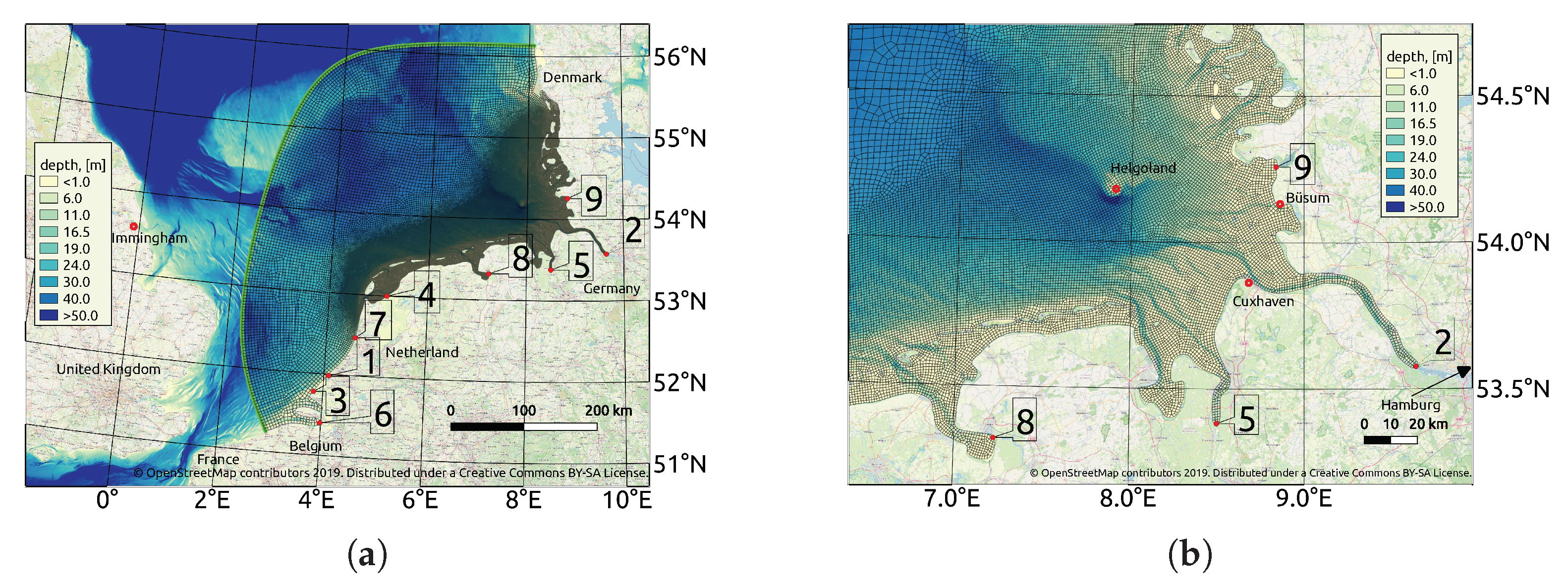
2.1. Bathymetry and Mesh
2.2. Boundary Conditions and Atmospheric Forcing
2.3. Initial Conditions and Spin-Up Period
2.4. Rivers
3. Simulation Results
3.1. Tidal Dynamics
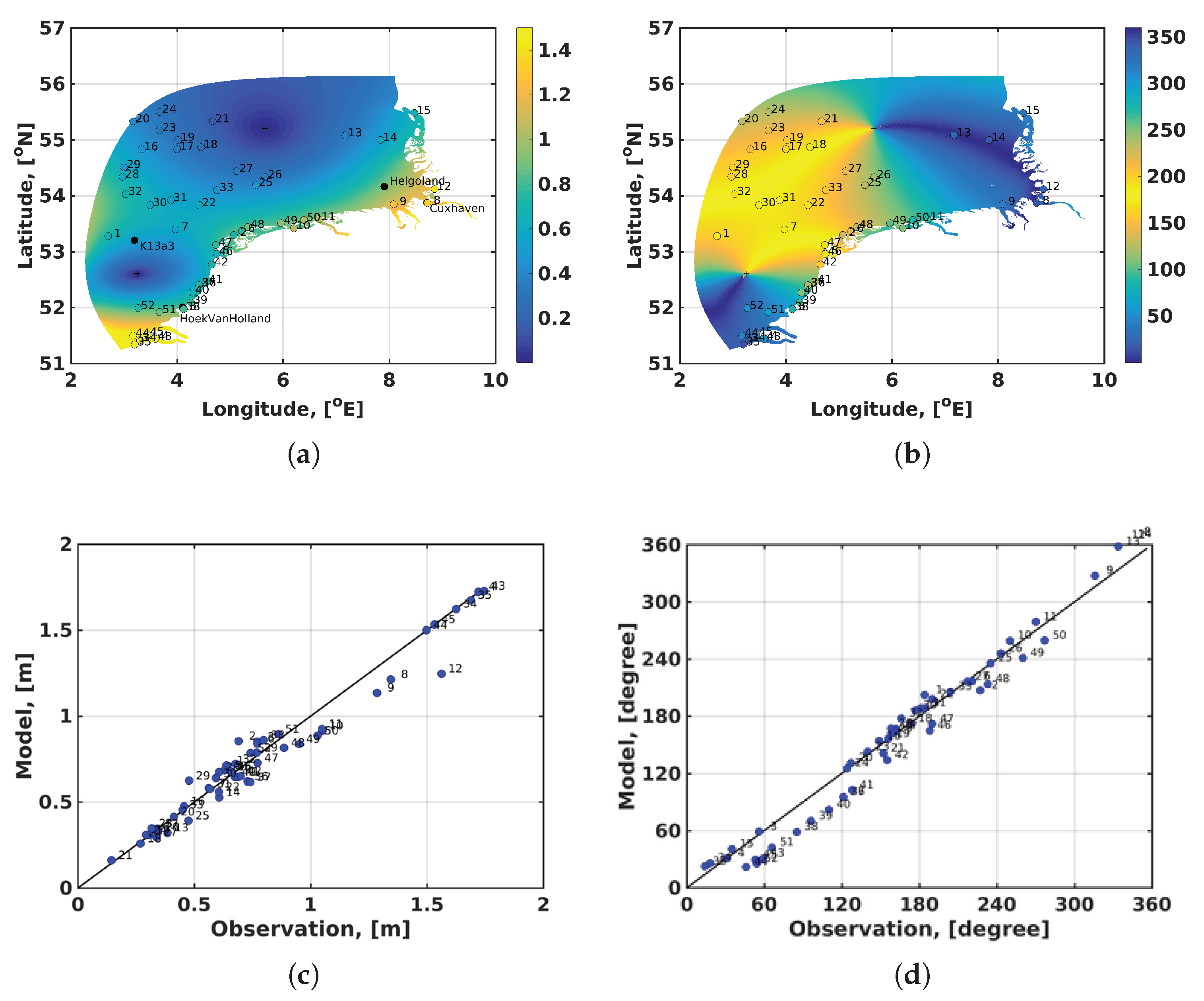
3.2. M2 Tide
3.3. Main Tidal Harmonics on Long Time Scales
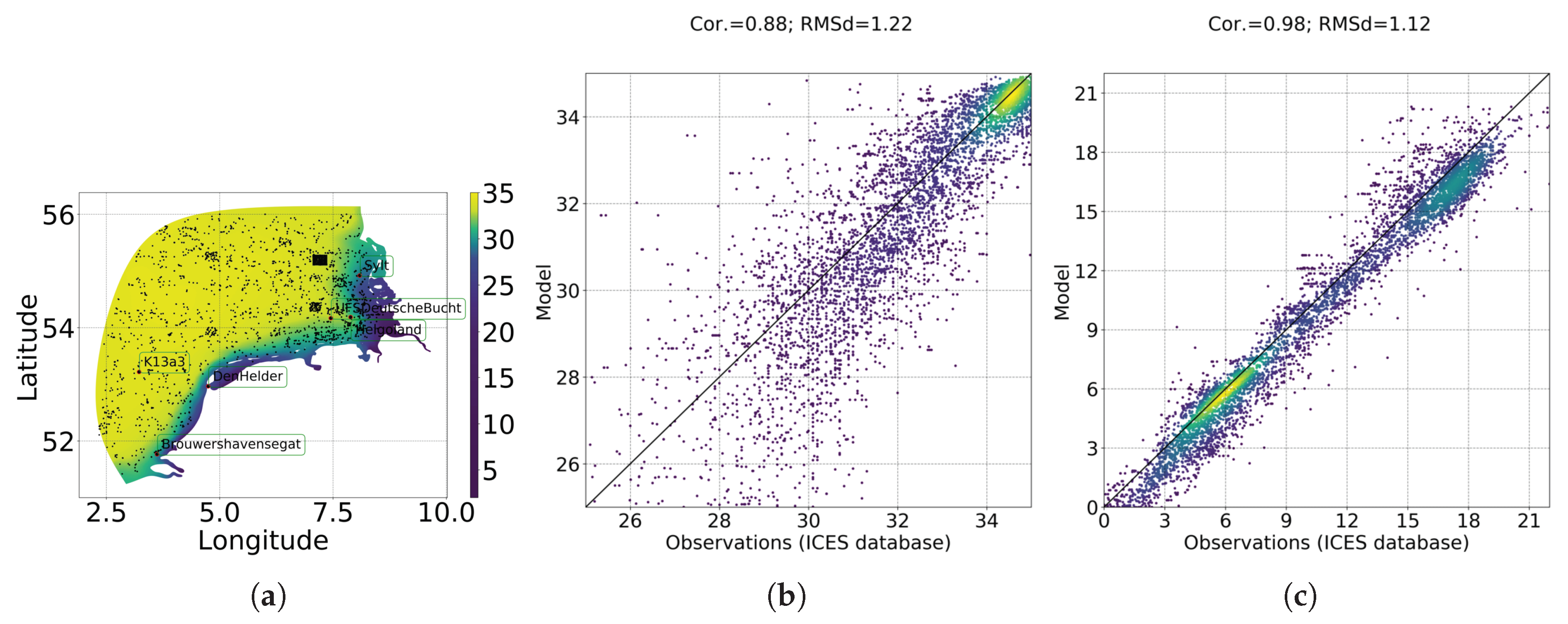
3.4. Surface Salinity and Temperature over 2010–2014
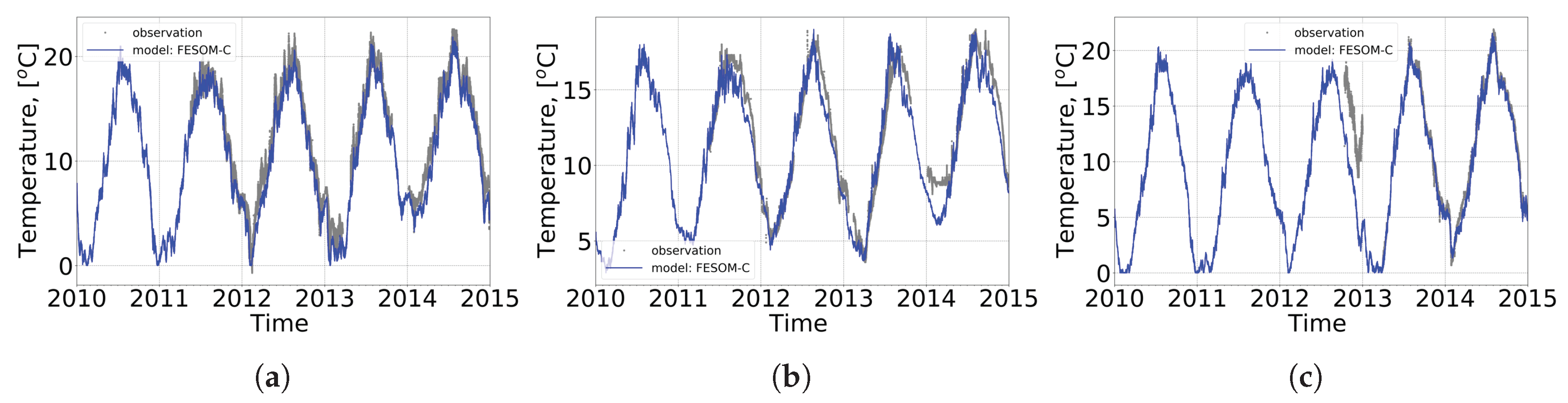
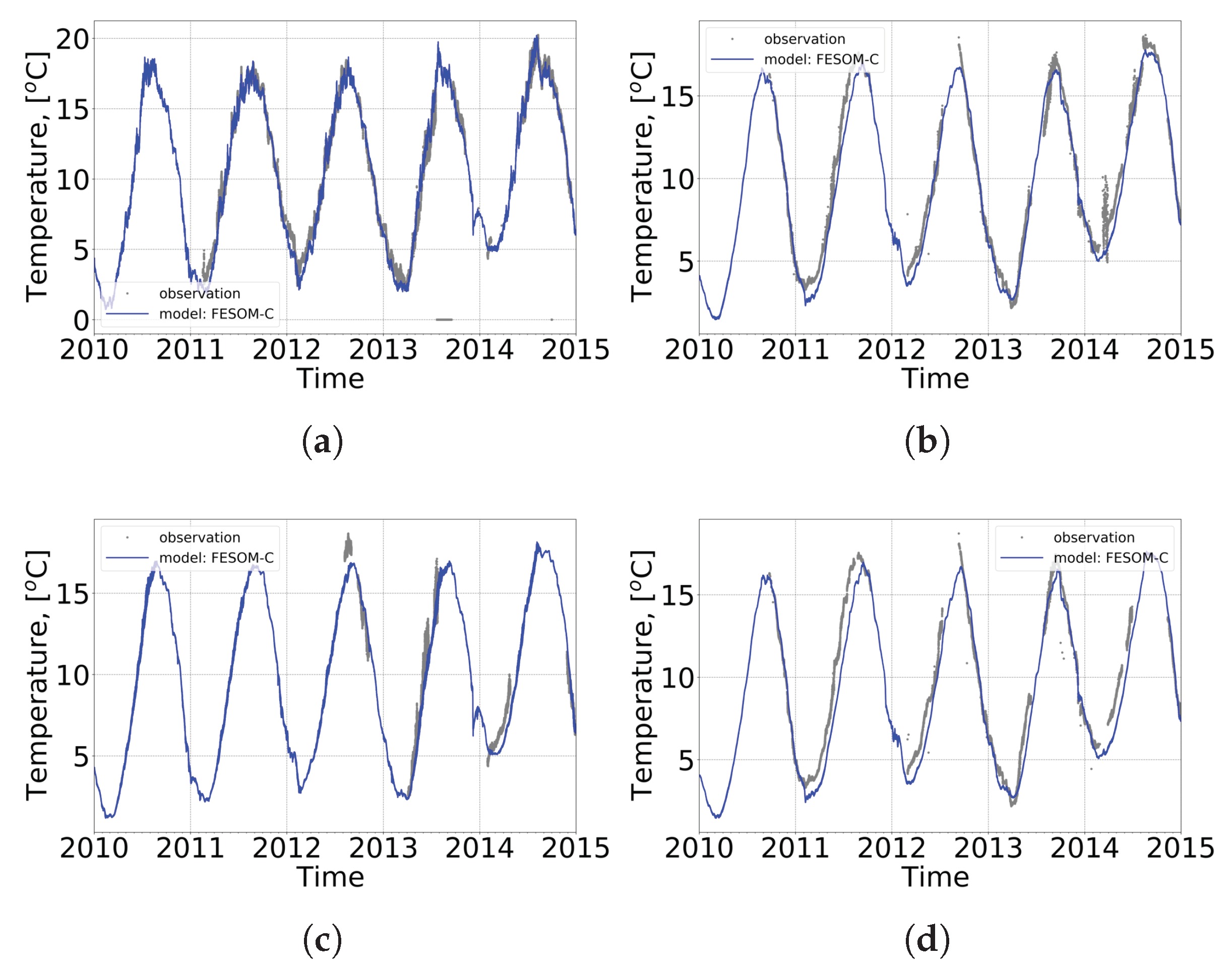
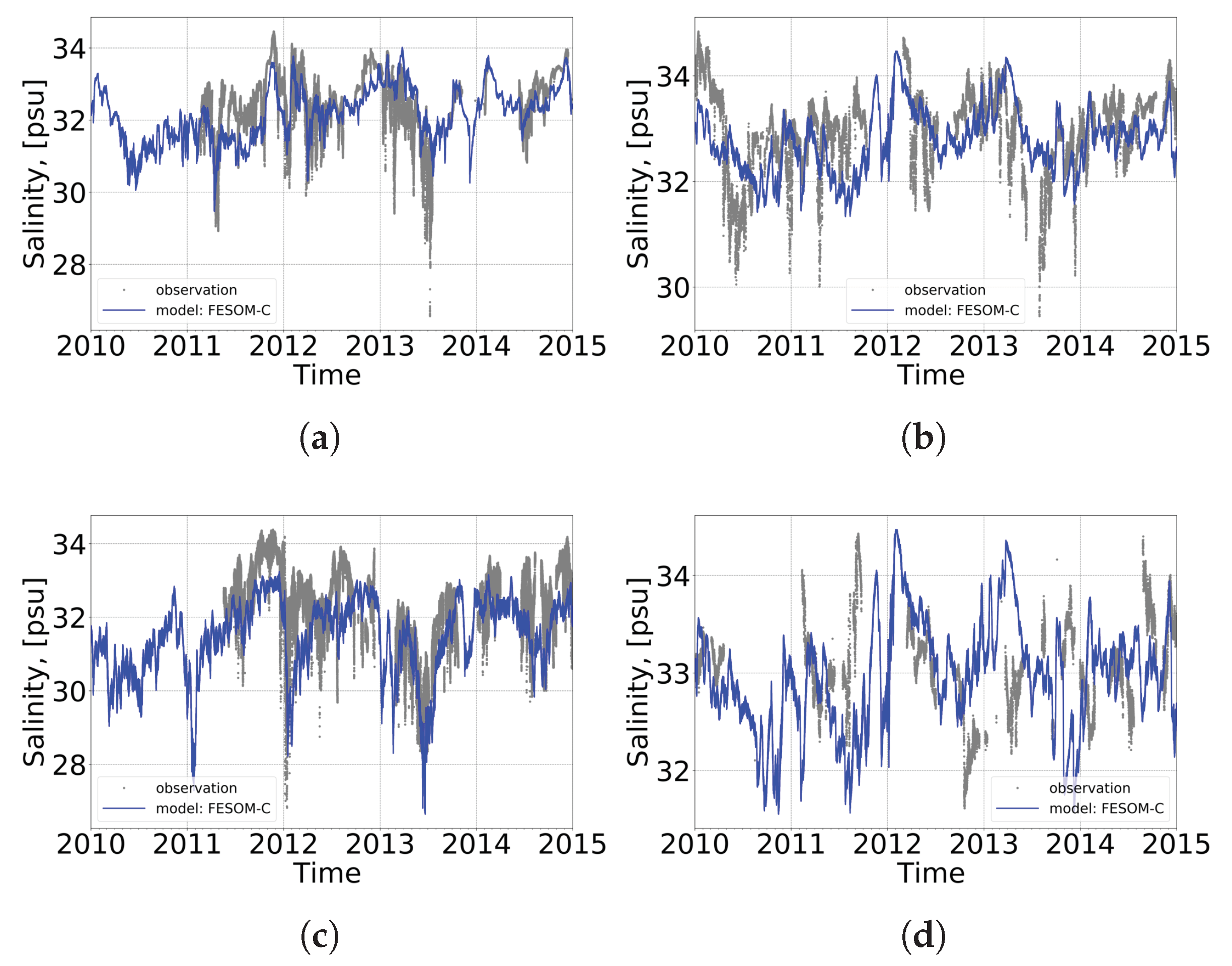
3.5. Time Series of Temperature and Salinity
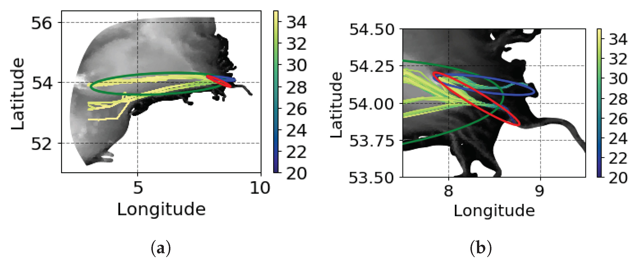
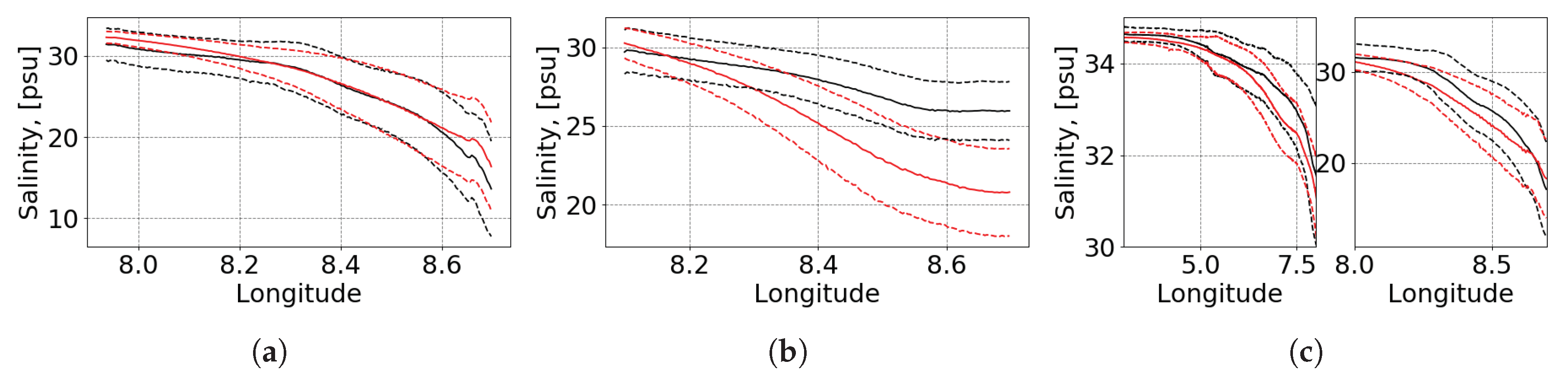
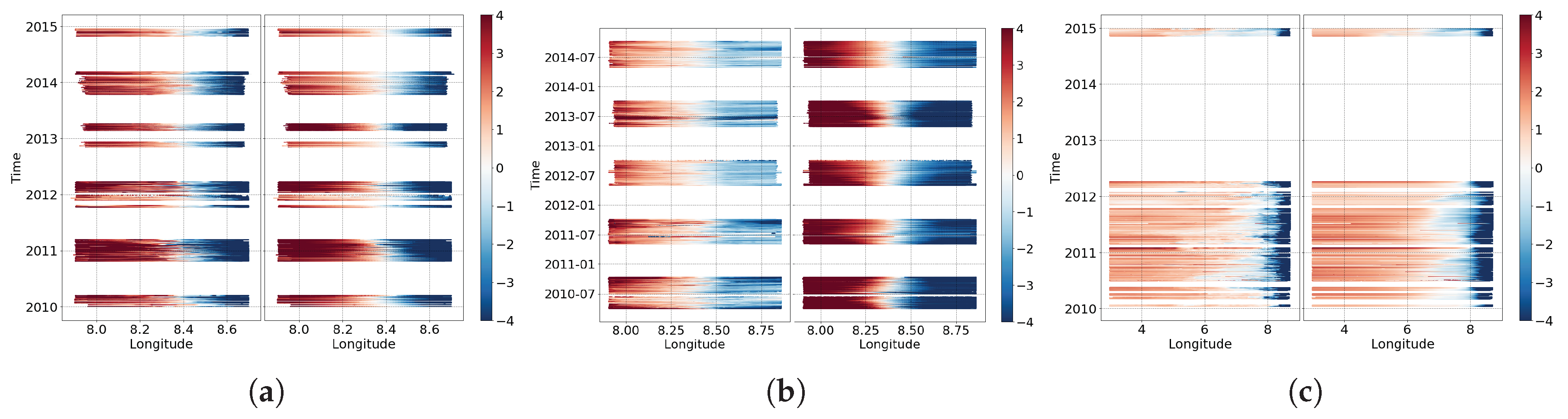
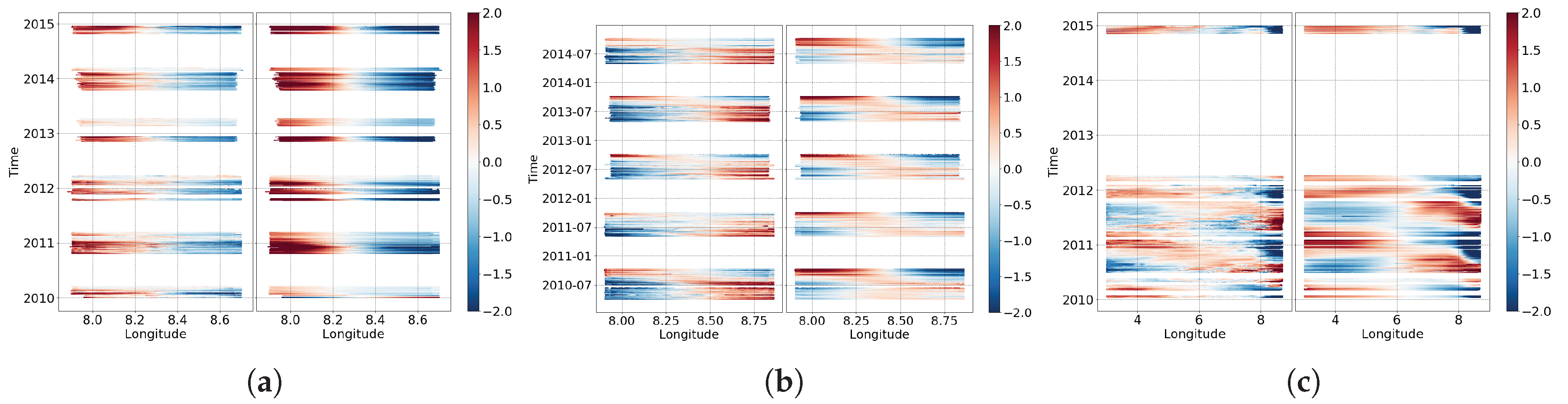
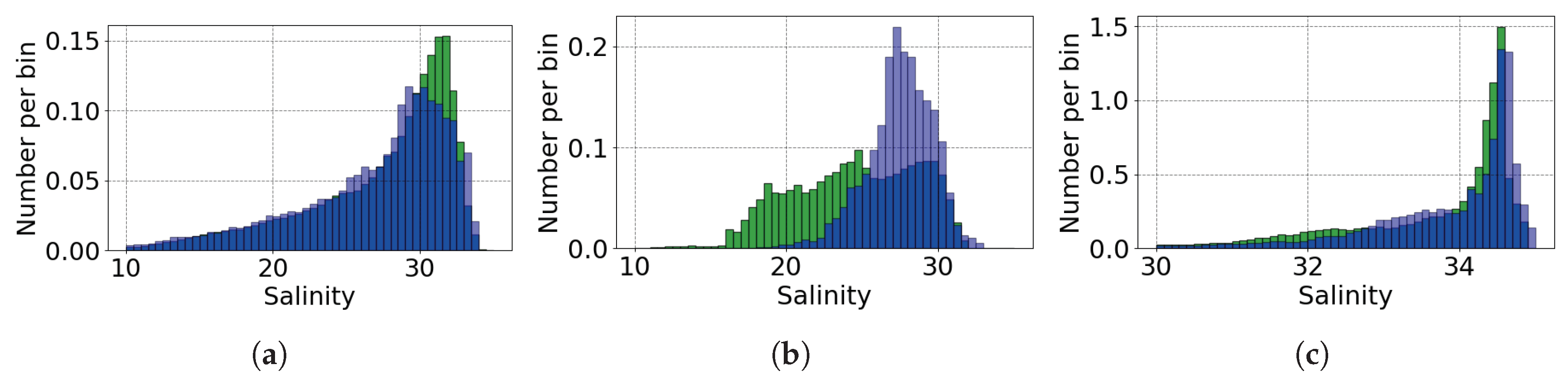
3.6. Salinity and Temperature, Ferry Lines
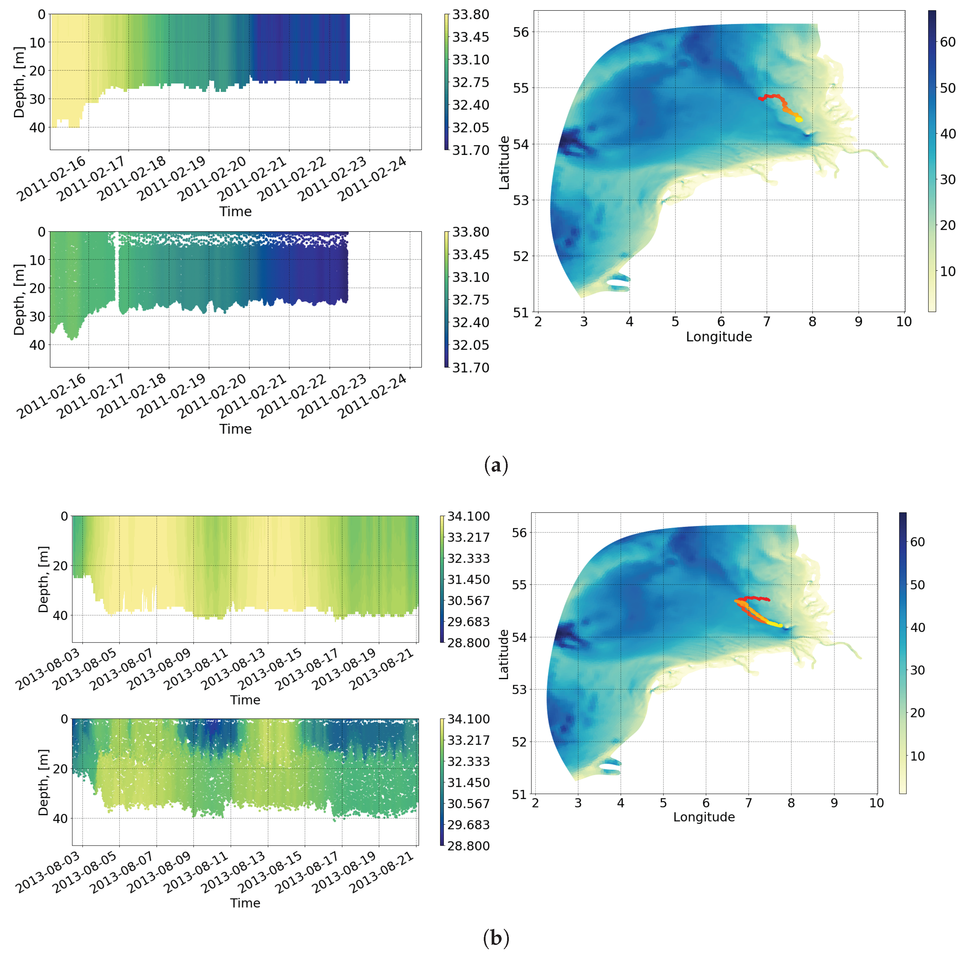
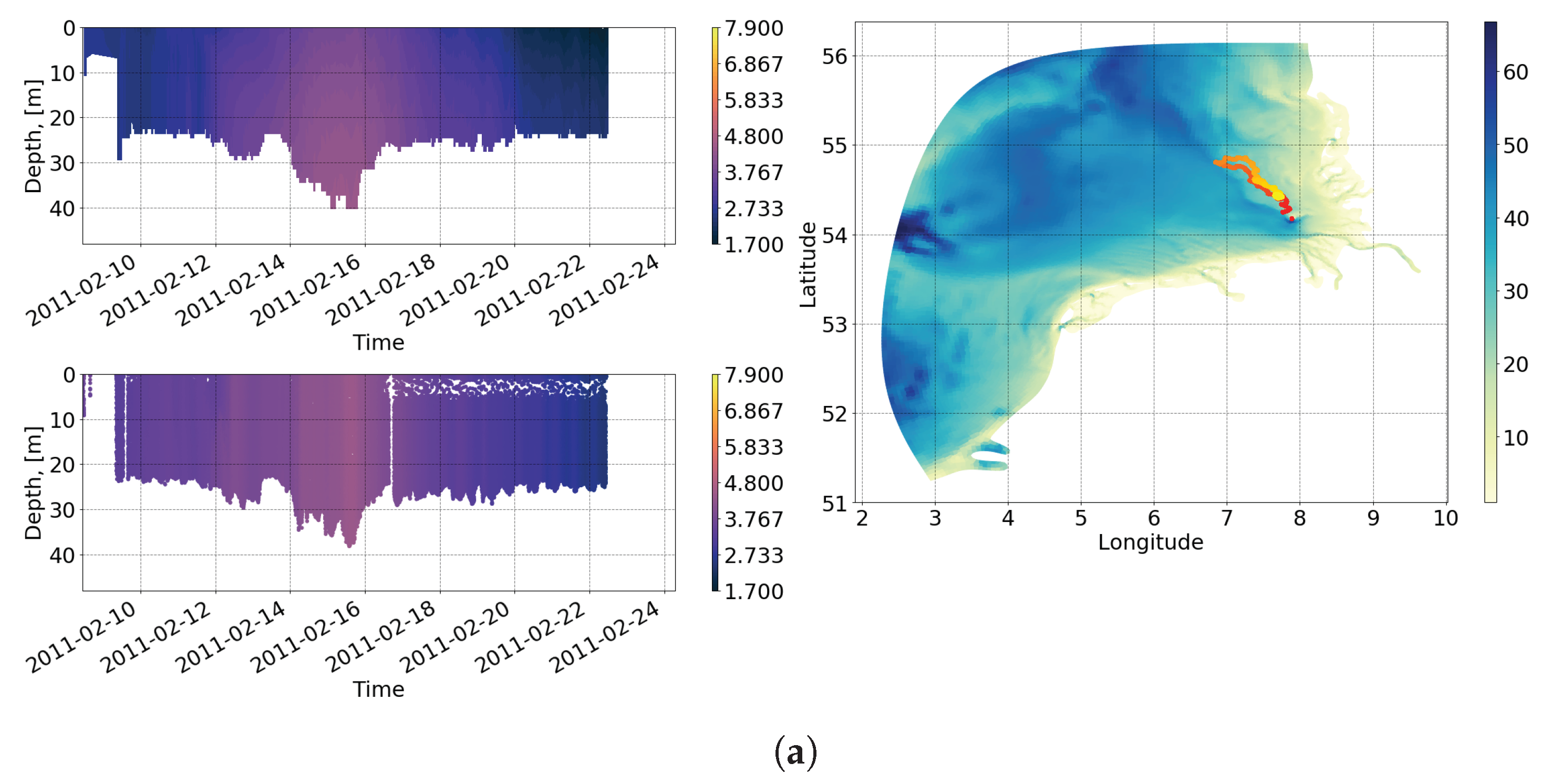
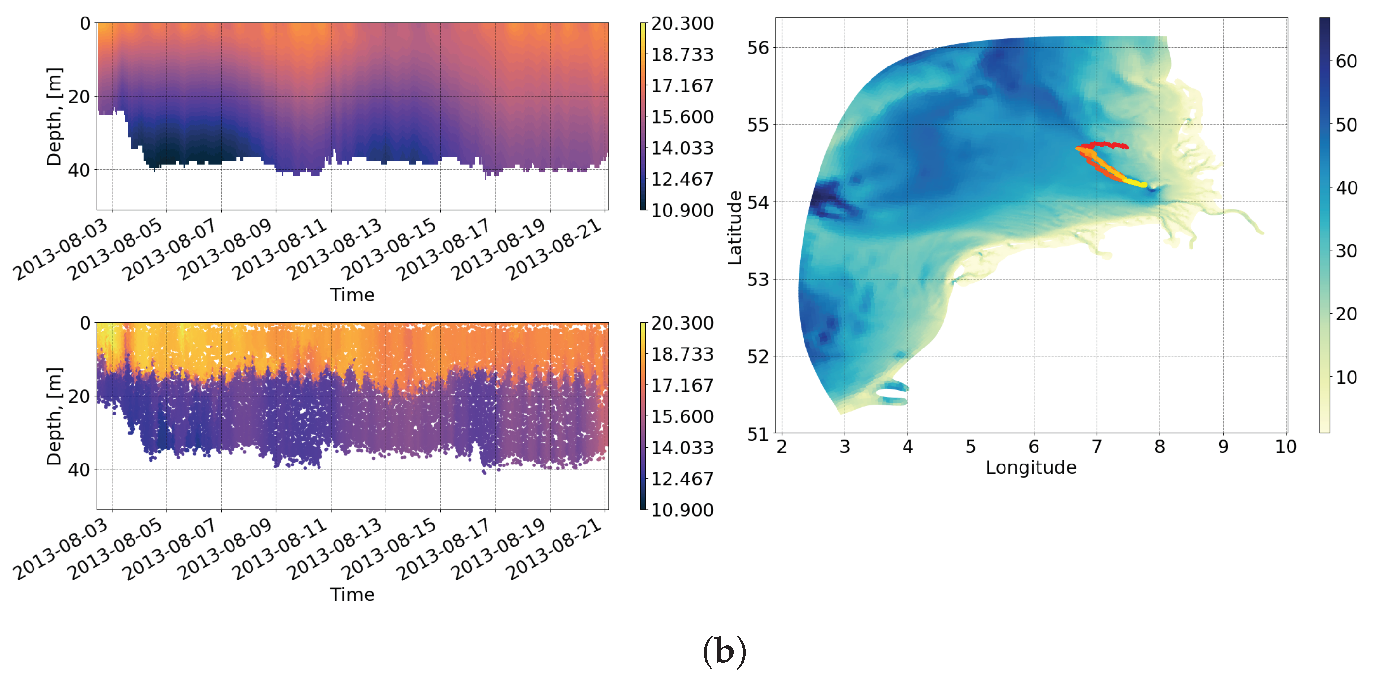
3.7. Vertical Structure, Gliders
4. Discussion, Mesh Resolution
Solution Convergence on Different Meshes
5. Conclusions
6. Code Availability
Author Contributions
Funding
Acknowledgments
Conflicts of Interest
References
- Danilov, S.; Sidorenko, D.; Wang, Q.; Jung, T. The finite-volume sea ice-Ocean model (FESOM2). Geosci. Model Dev. 2017, 10, 765–789. [Google Scholar] [CrossRef]
- Madec, G.; The NEMO System Team. NEMO Ocean Engine, Version 3.6 Stable; Technical Report 27; note du Pôle de modélisation de l’Institut Pierre-Simon Laplace No 27; IPSL, 2015; Available online: http://www.nemo-ocean.eu/ (accessed on 14 May 2020).
- Shchepetkin, A.F.; McWilliams, J.C. The regional oceanic modeling system (ROMS): A split-explicit, free-surface, topography-following-coordinate oceanic model. Ocean Model. 2005, 9, 347–404. [Google Scholar] [CrossRef]
- Griffies, S.M. Elements of the Modular Ocean Model (MOM): 2012 Release; Technical Report C; NOAA/Geophysical Fluid Dynamics Laboratory: Princeton, NJ, USA, 2012. [Google Scholar]
- Burchard, H.; Bolding, K. Getm—A General Estuarine Transport Model. Scientific Documentation; Technical report EUR 20253 en; European Commission, Joint Research Centre, Institute for Environment and Sustainability: Copenhagen, Denmark, 2002; p. 164. [Google Scholar]
- Chen, C.; Huang, H.; Beardsley, R.C.; Liu, H.; Xu, Q.; Cowles, G. A finite volume numerical approach for coastal ocean circulation studies: Comparisons with finite difference models. J. Geophys. Res. Ocean. 2007, 112. [Google Scholar] [CrossRef]
- Izquierdo, A.; Mikolajewicz, U. The role of tides in the spreading of Mediterranean Outflow waters along the southwestern Iberian margin. Ocean Model. 2019, 133, 27–43. [Google Scholar] [CrossRef]
- Murray, S.P.; Arief, D. Throughflow into the Indian Ocean through the Lombok Strait, January 1985–January 1986. Nature 1988, 333, 444–447. [Google Scholar] [CrossRef]
- Marchesiello, P.; McWilliams, J.C.; Shchepetkin, A. Open boundary conditions for long-term integration of regional oceanic models. Ocean Model. 2001, 3, 1–20. [Google Scholar] [CrossRef]
- Marsaleix, P.; Auclair, F.; Estournel, C. Considerations on open boundary conditions for regional and coastal ocean models. J. Atmos. Ocean. Technol. 2006, 23, 1604–1613. [Google Scholar] [CrossRef]
- Gräwe, U.; Flöser, G.; Gerkema, T.; Duran-Matute, M.; Badewien, T.H.; Schulz, E.; Burchard, H. A numerical model for the entire Wadden Sea: Skill assessment and analysis of hydrodynamics. J. Geophys. Res. Ocean. 2016, 121, 5231–5251. [Google Scholar] [CrossRef]
- Weisse, R.; Bisling, P.; Gaslikova, L.; Geyer, B.; Groll, N.; Hortamani, M.; Matthias, V.; Maneke, M.; Meinke, I.; Meyer, E.M.; et al. Climate services for marine applications in Europe. Earth Perspect. 2015, 2. [Google Scholar] [CrossRef]
- Debreu, L.; Marchesiello, P.; Penven, P.; Cambon, G. Two-way nesting in split-explicit ocean models: Algorithms, implementation and validation. Ocean Model. 2012, 49–50, 1–21. [Google Scholar] [CrossRef]
- Herzfeld, M.; Rizwi, F. A two-way nesting framework for ocean models. Environ. Model. Softw. 2019, 117, 200–213. [Google Scholar] [CrossRef]
- Sheng, J.; Greatbatch, R.; Zhai, X.; Tang, L. A new two-way nesting technique for ocean modeling based on the smoothed semi-prognostic method. Ocean Dyn. 2005, 55, 162–177. [Google Scholar] [CrossRef]
- Chen, C.; Liu, H.; Beardsley, R.C. An unstructured grid, finite-volume, three-dimensional, primitive equations ocean model: Application to coastal ocean and estuaries. J. Atmos. Ocean. Technol. 2003, 20, 159–186. [Google Scholar] [CrossRef]
- Qi, J.; Chen, C.; Beardsley, R.C. FVCOM one-way and two-way nesting using ESMF: Development and validation. Ocean Model. 2018, 124, 94–110. [Google Scholar] [CrossRef]
- Zhang, Y.J.; Ye, F.; Stanev, E.V.; Grashorn, S. Seamless cross-scale modeling with SCHISM. Ocean Model. 2016, 102, 64–81. [Google Scholar] [CrossRef]
- Zhang, Y.; Baptista, A.M. SELFE: A semi-implicit Eulerian-Lagrangian finite-element model for cross-scale ocean circulation. Ocean Model. 2008, 21, 71–96. [Google Scholar] [CrossRef]
- Burchard, H.; Schuttelaars, H.M.; Ralston, D.K. Sediment Trapping in Estuaries. Annu. Rev. Mar. Sci. 2017, 10, 371–395. [Google Scholar] [CrossRef]
- Fransner, F.; Nycander, J.; Mörth, C.M.; Humborg, C.; Markus Meier, H.E.; Hordoir, R.; Gustafsson, E.; Deutsch, B. Tracing terrestrial DOC in the Baltic Sea—A 3-D model study. Glob. Biogeochem. Cycles 2016, 30, 134–148. [Google Scholar] [CrossRef]
- Hordoir, R.; Axell, L.; Höglund, A.; Dieterich, C.; Fransner, F.; Gröger, M.; Liu, Y.; Pemberton, P.; Schimanke, S.; Andersson, H.; et al. Nemo-Nordic 1.0: A NEMO-based ocean model for the Baltic and North seas—Research and operational applications. Geosci. Model Dev. 2019, 12, 363–386. [Google Scholar] [CrossRef]
- Hordoir, R.; Axell, L.; Löptien, U.; Dietze, H.; Kuznetsov, I. Influence of sea level rise on the dynamics of salt inflows in the Baltic Sea. J. Geophys. Res. Ocean. 2015, 120, 6653–6668. [Google Scholar] [CrossRef]
- Wekerle, C.; Wang, Q.; Danilov, S.; Schourup-Kristensen, V.; von Appen, W.J.; Jung, T. Atlantic Water in the Nordic Seas: Locally eddy-permitting ocean simulation in a global setup. J. Geophys. Res. Ocean. 2017, 122, 914–940. [Google Scholar] [CrossRef]
- Androsov, A.; Fofonova, V.; Kuznetsov, I.; Danilov, S.; Rakowsky, N.; Harig, S.; Brix, H.; Helen Wiltshire, K. FESOM-C v.2: Coastal dynamics on hybrid unstructured meshes. Geosci. Model Dev. 2019, 12, 1009–1028. [Google Scholar] [CrossRef]
- Fofonova, V.; Androsov, A.; Sander, L.; Kuznetsov, I.; Amorim, F.; Hass, H.C.; Wiltshire, K.H. Non-linear aspects of the tidal dynamics in the Sylt-Rømø Bight, south-eastern North Sea. Ocean Sci. 2019, 15, 1761–1782. [Google Scholar] [CrossRef]
- Danilov, S.; Androsov, A. Cell-vertex discretization of shallow water equations on mixed unstructured meshes. Ocean Dyn. 2015, 65, 33–47. [Google Scholar] [CrossRef]
- OSPAR Commission London. Quality Status Report 2010; Technical report; OSPAR Commission London: London, UK, 2010. [Google Scholar]
- Clark, S.; Schroeder, F.; Baschek, B. The Influence of Large Offshore Wind Farms on the North Sea And Baltic Sea—A Comprehensive Literature Review; Technical report; Helmholtz-Zentrum Geesthacht, Zentrum für Material-und Küstenforschung: Geesthacht, Germany, 2014. [Google Scholar]
- Sündermann, J.; Pohlmann, T. A brief analysis of North Sea physics. Oceanologia 2011, 53, 663–689. [Google Scholar] [CrossRef]
- Reise, K.; Baptist, M.; Burbridge, P.; Dankers, N.; Fischer, L.; Flemming, B.; Oost, A.P.; Smit, C. The Wadden Sea—A Outstanding Tidal Wetland. Wadden Sea Ecosystem No. 29; Technical Report 29; Common Wadden Sea Secretariat (CWSS): Wilhelmshaven, Germany, 2010. [Google Scholar]
- Stanev, E.V.; Schulz-Stellenfleth, J.; Staneva, J.; Grayek, S.; Grashorn, S.; Behrens, A.; Koch, W.; Pein, J. Ocean forecasting for the German Bight: From regional to coastal scales. Ocean Sci. 2016, 12, 1105–1136. [Google Scholar] [CrossRef]
- Haller, M.; Janssen, F.; Siddorn, J.; Petersen, W.; Dick, S. Evaluation of numerical models by FerryBox and fixed platform in situ data in the southern North Sea. Ocean Sci. 2015, 11, 879–896. [Google Scholar] [CrossRef]
- Purkiani, K.; Becherer, J.; Flöser, G.; Gräwe, U.; Mohrholz, V.; Schuttelaars, H.M.; Burchard, H. Numerical analysis of stratification and destratification processes in a tidally energetic inlet with an ebb tidal delta. J. Geophys. Res. Ocean. 2015, 120, 225–243. [Google Scholar] [CrossRef]
- Stanev, E.V.; Pein, J.; Grashorn, S.; Zhang, Y.; Schrum, C. Dynamics of the Baltic Sea straits via numerical simulation of exchange flows. Ocean Model. 2018, 131, 40–58. [Google Scholar] [CrossRef]
- Zhang, Y.J.; Stanev, E.; Grashorn, S. Unstructured-grid model for the North Sea and Baltic Sea: Validation against observations. Ocean Model. 2016, 97, 91–108. [Google Scholar] [CrossRef]
- Pein, J.U.; Stanev, E.V.; Zhang, Y.J. The tidal asymmetries and residual flows in Ems Estuary. Ocean Dyn. 2014, 64, 1719–1741. [Google Scholar] [CrossRef]
- Shom. Shom (Service Hydrographique et Océanographique de la Marine) (2018). EMODnet Digital Bathymetry (DTM 2018). 2018. Available online: https://sextant.ifremer.fr/record/18ff0d48-b203-4a65-94a9-5fd8b0ec35f6/ (accessed on 12 May 2020).
- Geuzaine, C.; Remacle, J.F. Gmsh: A 3-D finite element mesh generator with built-in pre- and post-processing facilities. Int. J. Numer. Methods Eng. 2009, 79, 1309–1331. [Google Scholar] [CrossRef]
- Remacle, J.F.; Lambrechts, J.; Seny, B.; Marchandise, E.; Johnen, A.; Geuzainet, C. Blossom-Quad: A non-uniform quadrilateral mesh generator using a minimum-cost perfect-matching algorithm. Int. J. Numer. Methods Eng. 2012, 89, 1102–1119. [Google Scholar] [CrossRef]
- Nú nez-Riboni, I.; Akimova, A. Monthly maps of optimally interpolated in situ hydrography in the North Sea from 1948 to 2013. J. Mar. Syst. 2015, 151, 15–34. [Google Scholar] [CrossRef]
- Egbert, G.D.; Erofeeva, S.Y. Efficient inverse modeling of barotropic ocean tides. J. Atmos. Ocean. Technol. 2002, 19, 183–204. [Google Scholar] [CrossRef]
- Androsov, A.A.; Klevanny, K.A.; Salusti, E.S.; Voltzinger, N.E. Open boundary conditions for horizontal 2-D curvilinear-grid long-wave dynamics of a strait. Adv. Water Resour. 1995, 18, 267–276. [Google Scholar] [CrossRef]
- Ridal, M.; Olsson, E.; Unden, P.; Zimmermann, K.; Ohlsson, A. Deliverable D2.7: HARMONIE Reanalysis Report of Results and Dataset; Technical report; SMHI: North Köping, Sweden, 2017. [Google Scholar]
- Kerimoglu, O.; Hofmeister, R.; Maerz, J.; Riethmüller, R.; Wirtz, K.W. The acclimative biogeochemical model of the southern North Sea. Biogeosciences 2017, 14, 4499–4531. [Google Scholar] [CrossRef]
- Radach, G.; Pätsch, J. Variability of continental riverine freshwater and nutrient inputs into the North Sea for the years 1977-2000 and its consequences for the assessment of eutrophication. Estuaries Coasts 2007, 30, 66–81. [Google Scholar] [CrossRef]
- Voynova, Y.G.; Brix, H.; Petersen, W.; Weigelt-Krenz, S.; Scharfe, M. Extreme flood impact on estuarine and coastal biogeochemistry: The 2013 Elbe flood. Biogeosciences 2017, 14, 541–557. [Google Scholar] [CrossRef]
- Valle-Levinson, A.; Stanev, E.; Badewien, T.H. Tidal and subtidal exchange flows at an inlet of the Wadden Sea. Estuarine Coast. Shelf Sci. 2018, 202, 270–279. [Google Scholar] [CrossRef]
- Stanev, E.V.; Al-Nadhairi, R.; Valle-Levinson, A. The role of density gradients on tidal asymmetries in the German Bight. Ocean Dyn. 2015, 65, 77–92. [Google Scholar] [CrossRef]
- Codiga, D.L. Unified Tidal Analysis and Prediction Using the UTide Matlab Functions; Technical report; Graduate School of Oceanography, University of Rhode Island: Narragansett, RI, USA, 2011. [Google Scholar] [CrossRef]
- Baschek, B.; Schroeder, F.; Brix, H.; Riethmüller, R.; Badewien, T.H.; Breitbach, G.; Brügge, B.; Colijn, F.; Doerffer, R.; Eschenbach, C.; et al. The Coastal Observing System for Northern and Arctic Seas (COSYNA). Ocean Sci. 2017, 13, 379–410. [Google Scholar] [CrossRef]
- Bersch, M.; Gouretski, V.; Sadikni, R.; Hinrichs, I. KLIWAS North Sea Climatology of Hydrographic Data (Version 1.0). World Data Cent. Clim. (WDCC) 2013. [Google Scholar] [CrossRef]
- Purkiani, K.; Becherer, J.; Klingbeil, K.; Burchard, H. Wind-induced variability of estuarine circulation in a tidally energetic inlet with curvature. J. Geophys. Res. Ocean. 2016, 121, 3261–3277. [Google Scholar] [CrossRef]
- Becherer, J.; Stacey, M.T.; Umlauf, L.; Burchard, H. Lateral Circulation Generates Flood Tide Stratification and Estuarine Exchange Flow in a Curved Tidal Inlet. J. Phys. Oceanogr. 2014, 45, 638–656. [Google Scholar] [CrossRef]
- Petersen, W.; Schroeder, F.; Bockelmann, F.D. FerryBox—Application of continuous water quality observations along transects in the North Sea. Ocean Dyn. 2011, 61, 1541–1554. [Google Scholar] [CrossRef]
- Petersen, W. FerryBox systems: State-of-the-art in Europe and future development. J. Mar. Syst. 2014, 140, 4–12. [Google Scholar] [CrossRef]
- Grayek, S.; Staneva, J.; Schulz-Stellenfleth, J.; Petersen, W.; Stanev, E.V. Use of FerryBox surface temperature and salinity measurements to improve model based state estimates for the German Bight. J. Mar. Syst. 2011, 88, 45–59. [Google Scholar] [CrossRef]
- Dieterich, C.; Wang, S.; Schimanke, S.; Gröger, M.; Klein, B.; Hordoir, R.; Samuelsson, P.; Liu, Y.; Axell, L.; Höglund, A.; et al. Surface Heat Budget over the North Sea in Climate Change Simulations. Atmosphere 2019, 10, 272. [Google Scholar] [CrossRef]
- Koldunov, N.V.; Aizinger, V.; Rakowsky, N.; Scholz, P.; Sidorenko, D.; Danilov, S.; Jung, T. Scalability and some optimization of the Finite-volumE Sea ice-Ocean Model, Version 2.0 (FESOM2). Geosci. Model Dev. 2019, 12, 3991–4012. [Google Scholar] [CrossRef]


| River Name | Discharge [m/s] mean/min./max./std. |
|---|---|
| 1 Nieuwe Waterweg | 1408/11/4044/606 |
| 2 River Elbe | 783/261/4070/505 |
| 3 Haringvliet | 546/1/5903/817 |
| 4 Lake IJssel | 521/1/2935/402 |
| 5 River Weser | 269/87/1320/195 |
| 6 River Scheldt | 127/35/615/91 |
| 7 North Sea Canal | 84/1/365/41 |
| 8 River Ems | 70/20/372/52 |
| 9 River Eider | 23/12/40/6 |
| Station Name | Correlation | STD Observation | STD FESOM-C |
|---|---|---|---|
| Helgoland | 0.95 | 0.90 | 0.81 |
| Cuxhaven | 0.93 | 1.11 | 1.02 |
| Hoek van Holland | 0.91 | 0.67 | 0.7 |
| K13a3 | 0.89 | 0.47 | 0.42 |
| FerryBox (Operation Area) | Number of Measurements | Number of Transects | S, RMSE | T, RMSE | , RMSE |
|---|---|---|---|---|---|
| Cuxhaven–Helgoland | ≈234,000 | 583 | 1.7 (2.2) | 0.8 (2.7) | 1.3 (1.8) |
| Büsum–Helgoland | ≈502,000 | 1171 | 2.3 (3.8) | 0.7 (2.9) | 1.7 (2.5) |
| Cuxhaven–Immingham | ≈1,552,000 | 350 | 0.9 (1.0) | 0.6 (1.2) | 0.7 (0.7) |
© 2020 by the authors. Licensee MDPI, Basel, Switzerland. This article is an open access article distributed under the terms and conditions of the Creative Commons Attribution (CC BY) license (http://creativecommons.org/licenses/by/4.0/).
Share and Cite
Kuznetsov, I.; Androsov, A.; Fofonova, V.; Danilov, S.; Rakowsky, N.; Harig, S.; Wiltshire, K.H. Evaluation and Application of Newly Designed Finite Volume Coastal Model FESOM-C, Effect of Variable Resolution in the Southeastern North Sea. Water 2020, 12, 1412. https://doi.org/10.3390/w12051412
Kuznetsov I, Androsov A, Fofonova V, Danilov S, Rakowsky N, Harig S, Wiltshire KH. Evaluation and Application of Newly Designed Finite Volume Coastal Model FESOM-C, Effect of Variable Resolution in the Southeastern North Sea. Water. 2020; 12(5):1412. https://doi.org/10.3390/w12051412
Chicago/Turabian StyleKuznetsov, Ivan, Alexey Androsov, Vera Fofonova, Sergey Danilov, Natalja Rakowsky, Sven Harig, and Karen Helen Wiltshire. 2020. "Evaluation and Application of Newly Designed Finite Volume Coastal Model FESOM-C, Effect of Variable Resolution in the Southeastern North Sea" Water 12, no. 5: 1412. https://doi.org/10.3390/w12051412
APA StyleKuznetsov, I., Androsov, A., Fofonova, V., Danilov, S., Rakowsky, N., Harig, S., & Wiltshire, K. H. (2020). Evaluation and Application of Newly Designed Finite Volume Coastal Model FESOM-C, Effect of Variable Resolution in the Southeastern North Sea. Water, 12(5), 1412. https://doi.org/10.3390/w12051412