Article

Simulating Reservoir Induced Lhasa Streamflow Variability Using ArcSWAT

State Key Laboratory of Water Resources and Hydropower Engineering Science, Wuhan University, Wuhan 430072, China
*
Author to whom correspondence should be addressed.
Water 2020, 12(5), 1370; https://doi.org/10.3390/w12051370
Submission received: 24 March 2020 / Revised: 7 May 2020 / Accepted: 8 May 2020 / Published: 12 May 2020
(This article belongs to the Section Hydrology)

Abstract

:
Lhasa River Basin being the socio-economic hotspot of Qinghai-Tibetan Plateau is experiencing an increased hydropower capacity in the form of damming and reservoir construction. The Pangduo hydropower station, commenced in 2013, is one of these developments. Lhasa River discharge is analyzed for spatial variability under the reservoir operation at Pondo and Lhasa gauging station. The Mann–Kendall Trend analysis reveals an increased precipitation and a decreased Lhasa River discharge trend upstream and downstream the reservoir. However, the discharge received at Lhasa gauging station is experiencing a greater decline revealed by Sen’s slope estimator. Soil and Water Assessment Tool (SWAT) modelling of the Lhasa River discharge for both the hydrometric stations from 2008–2016 reveals better simulation results for Pondo hydrometric station in terms of R2, NSE and PBIAS values. The modelling results for Pondo station correspond comparatively well to the reservoir operation procedures including water level and inflow despite of data availability constraint. However, the importance of non-simulated processes (e.g., groundwater abstractions) to the accurate prediction of the Lhasa flow regime particularly at the downstream flow gauge is recommended. The study can prove beneficial for local water distribution measures in Lhasa River Basin.

1. Introduction

Damming and reservoir operation has extensively changed the flow regimes of the rivers far and wide all over the world [1]. A rising number of dams have been put into operation over the world to encounter public water stresses [2,3]. According to statistical data, there are over 45,000 dams higher than 15 m globally [4]. Being the second leading renewable energy resource and chief source of renewable energy in the electricity division, hydropower has a momentous capability to lessen anthropogenic greenhouse gas emissions. In 2012, hydropower was assessed to count for approximately 3.8% of the world’s major energy consumption and endow approximately 16.5% to the global electricity supply [5,6]. By the end of 2013, the total global installed hydropower capacity augmented to 1000 GW, producing an annual power generation of 3750 TWh [5]. Therefore, understanding of dam conception and its regulating outcomes on river discharge is fundamental for river and watershed management and re-establishment.
China is presently the fastest emerging economy and leading developing country with substantial energy utilization. To meet its goal of reducing carbon dioxide emissions per unit of gross domestic product (GDP) by 40%–45% before 2020, China will have to increase its efforts to develop hydropower. Therefore, China decided to create eight of the 13 planned hydropower bases, i.e., Jinsha River, Lancang River, Dadu River, Upper Huanghe River, Yalong River, Nu River, mainstream Changjiang River, and Middle Yarlung Tzangbo River (Lhasa River investigated in this study is one of its tributaries), during 2011–2015 and further develop its installed conventional hydropower capacity to 420 GW by 2020, which includes the current conventional hydropower of 350 GW [7].
Watersheds function as a system comprising of components including stream flow received at the watershed outlet, evapotranspiration and anthropogenic water usage for urban and agricultural purposes [8,9,10]. For this reason, hydrological models have been established for mathematical illustration of hydrological processes, because they can improve the understanding of the impact of natural and anthropogenic interventions on hydrological features and forecast water resource changes, thus supporting decisions in water resource management [11,12,13]. In the recent advancements regarding water resource analysis, the evolution of remote sensing (RS) services and Geographic Information System (GIS) abilities has stimulated the expanded use of watershed models worldwide. It has supplemented in the precision of modeling by providing more concrete methods to define watershed conditions, delineating watershed characteristics, thus refining the modeling manner and eventually enhancing the assessment abilities of hydrological modeling [14]. Hydrological researchers are applying these models to understand the factors governing the runoff processes in diverse catchments around the world, e.g., snowmelt runoff process in northern Pakistan has been investigated by [15] using satellite data in Snowmelt Runoff Model (SRM). Similarly, many studies have utilized the Soil and Water Assessment Tool (SWAT) to simulate water cycle dynamics in response to management practices across the watershed and regional scales [16] such as the United States, the European Union [17], India [18], Australia [19], Africa [20] and China [21].
Construction of dams and reservoirs has generous impacts on the magnitude and variability of downstream runoff [22,23]. There are numerous techniques that have been applied to detect potential changes in streamflow, such as the Mann–Kendall test, Bayesian inference, and Pettitt test [24]. These changes can be associated to anthropogenic activities, such as the construction of reservoirs and dams, streamflow regulation, the rapid increase of water consumption [25,26,27]. However, the periodic variations of streamflow due to human activities received less attention, even though they play a vital role in regional water supply and hydropower generation [28,29]. Therefore, trustworthy demonstration of reservoir operations in hydrological models is critical for credible simulation of water cycling [19]. In this regard, [30] investigated the impact of reservoir on the Guadiana streamflow regime upstream and downstream the reservoir. SWAT model was applied in the Southern China province of Guangdong over the Dongjiang River watershed for simulating monthly river discharge at different hydrological stations upstream, down the nearest reservoir, in order to investigate hydrological drought propagation using Streamflow Simulation Index (SSI) [31], given that water shortages are experienced, and the mainstream hydrological behavior in this basin is affected by reservoir operation [32,33]. Therefore, the current study aims at (a) quantifying how reservoir operation influences watershed streamflow spatially, i.e., upstream and downstream the reservoir in Lhasa River Basin (henceforth LRB) and (b) conducting SWAT modelling of the regulated Lhasa River streamflow. The study aids in decision-making pertaining to influences of reservoir functioning and water distribution across different parts of the watershed.

2. Materials and Methods

2.1. Study Area

The Lhasa River, originating in the central western Qinghai-Tibetan Plateau in the Tibet Autonomous Region, is one of the major tributaries of the Yarlung Tsangbo River [34] with a total basin area of ≈32,321 km2 (as calculated by ArcSWAT in the current study), lying in a geographical range from WGS84-Lat 90°05′–93°20′ E; Lon 29°20′–31°15′ N (Figure 1) in south China, and functions as a center of political affairs, economy, culture, traffic and religion in Tibet Autonomous Region. The elevation in the basin ranges from 3560 m a.s.l. to 7097 m a.s.l. (from Study area Digital Elevation Model, Figure 1) with temperate semi-arid monsoon climate receiving abundant sunlight where the average minimum and maximum temperatures are about −1.7 to 9.7 °C. The Lhasa River Basin has three meteorological stations situated within the boundary of the basin naming Damxung, Maizhokunggar and Lhasa (Figure 1) providing long-term recorded data on the climate variables. The study area has three hydrological stations located at Pondo, Tanggya, and Lhasa. The gauging stations have a long time series data available on river flow.
The hydrological regime of Lhasa River is a decent illustration of rain dominated regime as approximately 90% of runoff is generated by the summer monsoon rains, specifically in the months of June–September resulting in the major high peak flows in Lhasa River during the same time period. The mean annual discharge and average annual precipitation in the area are about 237 m3/s and 460 mm, respectively.
In recent times, Lhasa River Basin has seen some major advancements regarding water resource management in the form of reservoir development and hydrological structures to utilize the water resource for progress of the area. The Zhikong and Pangduo hydropower stations and reservoirs have been built on Lhasa River in 2006 and 2013, respectively. The 100 MW capacity Zhikong Hydropower Station lies between the middle and lower reaches of the Lhasa River, downstream from the 160 MW Pangduo Hydropower Station (Figure 1). In the current study, the influence of Pangduo reservoir is investigated on streamflow recorded at the two chosen hydrometric stations, Pondo station located near the reservoir in the upper reach and Lhasa station located downstream in the middle reach of Lhasa River (Figure 1).

The Pangduo Reservoir

The Pangduo Water Conservancy Project is located in the upper Lhasa River. The area controlled by the dam site is 16,370 cubic meters, with an annual runoff of 6.248 billion cubic meters, accounting for 49.8% and 58.52% of the Lhasa River Basin, respectively. The Pangduo water conservancy project is a key water conservancy construction project in the “Eleventh Five-Year Plan” of the Tibet Autonomous Region. It is also the largest water conservancy project that has been recently constructed and planned. The development task of the Pangduo water conservancy project is mainly irrigation and power generation, taking into account both flood control and water supply. It is the backbone control project of the Lhasa River Basin and a leading reservoir for the elevator-level development of the Lhasa River Basin. The details of Pangduo reservoir are presents as Table 1.

2.2. Research Methodology

2.2.1. Mann–Kendall Trend Analysis on Hydrological Data

The study used trend analysis approach to define the hydrological behavior for the study area. The change quantification has been carried out focusing particularly on reservoir operation influence on the spatial variability of Lhasa River streamflow. The well-known Mann–Kendall (henceforth MK) Trend test [35] has been employed on the seasonal discharge of Lhasa River recorded at Pondo and Lhasa hydrometric stations. Seasonal discharge was put to trend analyses as the major proportion of river discharge is contributed in the summer months from June–September under the Indian Monsoon influence. The rank-based, non-parametric MK statistical test, which has presented strength in trend detection for non-normally distributed and censored data, such as the hydro-climatic data, was used for the flow trend analysis. The results of this test indicate the statistical significance of the observed variable trends where the sign corresponds to the sign of a trend. In this study, the significance level of p p < 0.05 (95% confidence level) was used to evaluate the change trends. In the MK test, the slope calculated using the Theil–Sen’s estimator is usually considered to represent the monotonic trend and indicates the amplitude of change per unit time. It is a robust estimate of the magnitude of a trend and has been widely used to identify the slope of the trend lines in hydrological and climatic time series.

2.2.2. SWAT Model Application

SWAT Model Description

SWAT is a physically based hydrological model developed by the US Department of Agriculture (USDA). SWAT is a distributed deterministic model that is extensively used to investigate the watershed hydrology [36,37]. Referring to [37] and [38], it is the optimum choice among the different hydrological models owing to its proficiency for application to large-scale watersheds (>100 km2), interface with a Geographic Information System (GIS), continuous-time simulations performance, and generation of the maximum number of sub-basins and ability to characterize the watershed in enough spatial detail. It is capable of simulating long term impacts of any management, climate or vegetation scenarios on the hydrological processes including pollution transport and sediment loading in river basins/watersheds [16]. SWAT model has emerged as one of the most widely used eco-hydrological models worldwide [39,40,41,42,43,44] (see Figure 2).
In SWAT model, a river basin or watershed is firstly partitioned into larger sub-units called sub-basins draining into the stream network and the river-system which are further distributed into a series of smaller units: the hydrological response units (HRUs), which are non-spatial uniform units, each signifying distinctive combinations of soil, land-use and slope. The calculations and simulations of hydrological components, sediment yield, and nutrient cycles are first carried for each HRU and then aggregated for the sub basins and watershed.
The hydrological cycle simulated in SWAT is based on the water balance equation:
S W t = S W 0 + i = 1 t R d a y Q s u r f E a w s e e p Q g w
where, S W 0 and S W t are the initial and final soil water content (mm H2O) on day i, t is time (days), R d a y is the precipitation amount reaching the soil surface on day i (mm H2O), Q s u r f   is the surface runoff amount on day i (mm H2O), E a is the evapo-transpiration on day i (mm H2O), w s e e p represents the interflow on day i (mm H2O), and Q g w is the return flow or base flow to the channel on day i (mm H2O).
The simulated hydrological components include infiltration; redistribution; evapotranspiration (ET); lateral subsurface flow; groundwater or return flow; surface runoff; ponds inflow and outflow; transmission losses and water yield. Further detailed background and theories of hydrological process in SWAT can be found in [45].

SWAT Model Input Datasets

In the current study, “ArcSWAT-2012, Rev. 634”, which is an ArcGIS-ArcView extension and graphical user input interface for SWAT model was prepared with the data, which requires three GIS data layers (digital elevation model (DEM), soils and land use) and the hydro-meteorological data of the study area. The topographic data of the study area was delivered in the form of a Digital Elevation Model (DEM) (Figure 1), acquired from Advanced Spaceborne Thermal Emission and Reflection Radiometer (ASTER)-Global Digital Elevation Model (GDEM) with a 3 arc-second (90 m) resolution provided with the watershed outlet point for stream network and watershed delineation by ArcSWAT.

Soil and Land Use Raster

The soil data was conveyed into ArcSWAT attained from FAO-UNESCO Harmonized World Soil Database version 1.2 (HWSD v1.2), a 30 arc-second raster database, with over 15,000 different soil mapping units, within the 1:5,000,000 scale FAO-UNESCO Soil Map of the World (www.fao.org/soils-portal) (Figure 3a).
The Land use raster was produced using Landsat-8 OLI satellite imagery with a 30 m resolution. Among images, the best cloud free image was selected to develop land use classification raster using Supervised Maximum Likelihood Classification method. (Figure 3b).

Hydro-Meteorological Data

For the current study, ArcSWAT model was fed with meteorological data on daily time step for climate variables including precipitation, maximum and minimum air temperature, relative humidity, wind speed and solar radiation obtained for a long-term period from Damxung, Maizhokunggar and Lhasa meteorological stations (Figure 1). The weather data were prepared in text file format as required by the SWAT model. The river discharge data used in the study was obtained from Pondo and Lhasa gauging stations (Figure 1).

Watershed Demarcation

In watershed delineation, we designated the outlet of the big watershed and let the software automatically generate the outlets of the sub-basins and delineate, therefore, each one of them. We set a threshold for the sub-basin area equal to 650 km2 to launch the sub-basin delineation. As a result, the study area was aligned with 21 sub-basins and 149 discrete HRUs (10%–15%–10% land use-soil-slope threshold), based on the different soils, land-use and slope classes.

2.2.3. Reservoir Addition to the Model

After the watershed delineation was achieved, Pangduo Reservoir was added to the SWAT model. Using the built-in reservoir module of SWAT model, Lhasa River streamflow was simulated against observed streamflow at the Pondo and Lhasa hydrological stations (Figure 1). SWAT model required data for the following parameters of reservoir:
(a)
Reservoir commencement year;
(b)
Volume of water required to fill the reservoir principal spillway (Table 1);
(c)
Volume of water required to fill the reservoir emergency spillway (Table 1);
(d)
Reservoir surface area.

2.2.4. Model Calibration, Validation and Sensitivity Analysis

To appraise the effect of reservoir operation on the flow regime, the observed monthly river flow from two gauging stations, i.e., Pondo and Lhasa was fed into the model to simulate the river flow for both the selected hydrometric sites individually. The SWAT model was applied for the simulation period of 1 January 2008, through 31 December 2016, with 2008–2009 as a warm-up period. A warm-up period is required for all SWAT simulations, because initial values for surface residue, plant biomass, groundwater height, soil moisture and many other parameters are generally set to zero or default values. The stream flow data of 3 years from 2010 to 2012 were used for calibration, and the succeeding 4 years from 2013–2016 were then used as validation period, which includes the reservoir functioning years for the study area.
Sensitivity analysis designates how model output fluctuates over a range of given input variables. This process confines the number of model parameters to the most sensitive ones that have a major influence on calibration of hydrological models for a given catchment. During this process, first perceptible ranges are assigned to a set of calibration parameters, where both the ranges and the selection of calibration parameter are guided by literature, specific knowledge of the study area and the parameters sensitivity analysis. After it is completed, sets of samples (as many as intended simulations) are built from the parameter ranges through Latin hypercube sampling, followed by SWAT model simulation using each of the set, and processed for selected objective function. The different techniques to perform sensitivity analysis can be generally grouped into local and global methodologies. Sampling one input at a time by setting all other inputs at constant values does not justify for the interaction between inputs. The global sensitivity, on the contrary, explores the whole range of input factors, and all input factors can be at once varied, permitting for an examination of output variation as a result of all inputs and possible interaction, where output uncertainty is averaged over all input factors. Commonly, hydrological model uncertainty can arise from input data, model parameterization and model structure. Khoi et al. 2015 [46] evaluated four SWAT model parameter uncertainty analysis approaches in simulating stream flow in the Srepok River watershed, Vietnam and resolved that the Sequential Uncertainty Fitting (SUFI-2) [47] method had the best performance. Therefore, for the current study, the SWAT-CUP (calibration and uncertainty program) embedded program SUFI-2 (Sequential Uncertainty Fitting version 2) was used for sensitivity analysis, calibration and validation of the model. This algorithm is adept at mapping all uncertainties (parameter, inputs, conceptual model, etc.) in terms of parameter ranges by attempting to enclose most of the measured data within the 95% prediction uncertainty (95PPU) band, which is calculated at the 2.5% and 97.5% levels of the cumulative distribution of all simulated output values. Nine hydrological parameters (Table 2) were recognized sensitive through global sensitivity analysis [48] where stream flow data of 9 hydrological years (2008–2016) were used to simulate Lhasa river discharge. The model was run for 500 simulations individually during the calibration and validation for both the hydrometric stations data. The settlement between observed and simulated catchment stream flow data was determined using subjective and quantitative measures for recommended parameter thresholds. The final value of each model parameter that showed optimal model efficiency during calibration was used for model validation without further adjustment Upon the achievement of sensitivity analysis for calibration and validation process of Lhasa River discharge; the most sensitive parameters were ranked in accordance with the t-stat and p-value assigned by SUFI-2 algorithm for the automatic calibration and validation of ArcSWAT model in the study area.

2.2.5. Model Evaluation Measures

To reckon the goodness of model performance for the carefully chosen ranges and parameter, in terms of calibration/uncertainty levels, two indices p-factor and the r-factor were used. P-factor is the percentage of data that is bracketed by the 95PPU band (range from 0 to 1, where 1 shows that all the prediction are within the 95PPU Band), while R-factor is the average width of the 95PPU band divided by the standard deviation of the measured variable (0 to , with 0 showing perfect match) [43]. For evaluation of calibration/validation results, the SUFI-2 algorithm allows users to select from a range of different objective functions such as R2, percent bias (PBIAS), Nash–Sutcliffe Efficiency (NSE) or Kling–Gupta efficiency (KGE). In general, the coefficient of determination (R2) and Nash–Sutcliffe Efficiency (NSE) are the most popular statistics used to evaluate the performance of the SWAT model [30,31,32,38]. The current study used R2 [49,50] as the main objective function, but the results were also evaluated based on, PBIAS and NSE [51] of the calibration/validation results as well as the P-factor and the R-factor.
The R2 is the magnitude of the linear relationship between the observed and the simulated values and was calculated as [52]:
R 2 = i = 1 n O i O ¯ S i S ¯ i = 1 n O i O ¯ 2 0.5 i = 1 n S i S ¯ 2 0.5 2
where Oi is the observed flow for the ith day of the simulation, Si is the modeled flow for the ith day of the simulation, O is the long term mean of the observed flow, and S is the long term mean of the simulated flows.
NSE is used to specify how accurate the plot of observed versus simulated value fits the 1:1 line, and was calculated as [51];
NSE = 1 i = 1 n Q i o b s Q i s i m 2 i = 1 n Q i o b s Q m e a n o b s 2
where Qiobs is the observed flow, Qisim is the simulated flow, and Qiobs mean is the average observed flow.
Percent bias (PBIAS) estimates the average tendency of the simulated values to be larger or smaller than their observed equivalents [53]. The best value of PBIAS is zero, signifying exact simulation of observed values. In general, a lower value of PBIAS implies accurate model simulation. PBIAS, which is the percent deviation of simulated data, is calculated as:
PBIAS = i = 1 n Q i o b s Q i s i m × 100 i = 1 n Q i o b s

3. Results

3.1. Hydrological Regime of Lhasa River

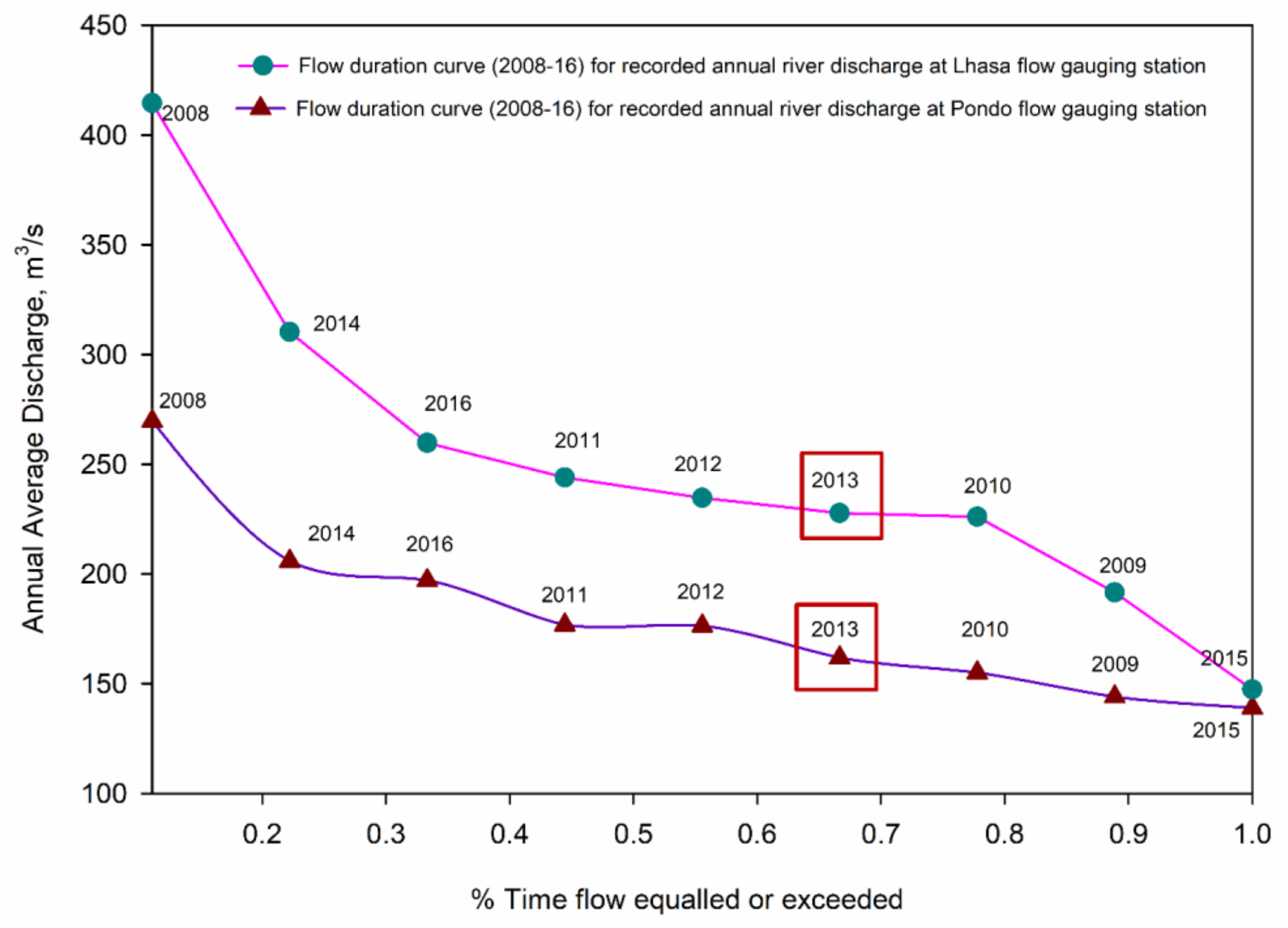
The magnitude of annual Lhasa River flow on a respective year and its exceeding probability for the time span of 2008–2016 recorded at Pondo flow gauge (near the chosen reservoir in the upper Lhasa River) and Lhasa flow gauge (downstream in the middle reach of Lhasa River) have been represented as flow-duration curves in Figure 4. The flow-duration curve is a cumulative frequency curve that shows the percent of time during which specified discharges are equaled or exceeded in a given period [54]. We see that the annual river discharge accumulated at Lhasa gauging station is higher as the magnitude of peak flow depends on the total basin area; the larger the basin area, the greater the resulting peak flow [55]. After the reservoir impoundment year (highlighted in Figure 4), the annual discharge for preceding years has increased. We see that the year 2015 has experienced the lowest annual discharge with maximum exceedance after the reservoir impoundment. This decreased annual flow can be attributed to a distinctively lower rainfall received during this year. Figure 4 indicates an identical behavioral pattern of annual Lhasa River discharge at both flow gauging stations.
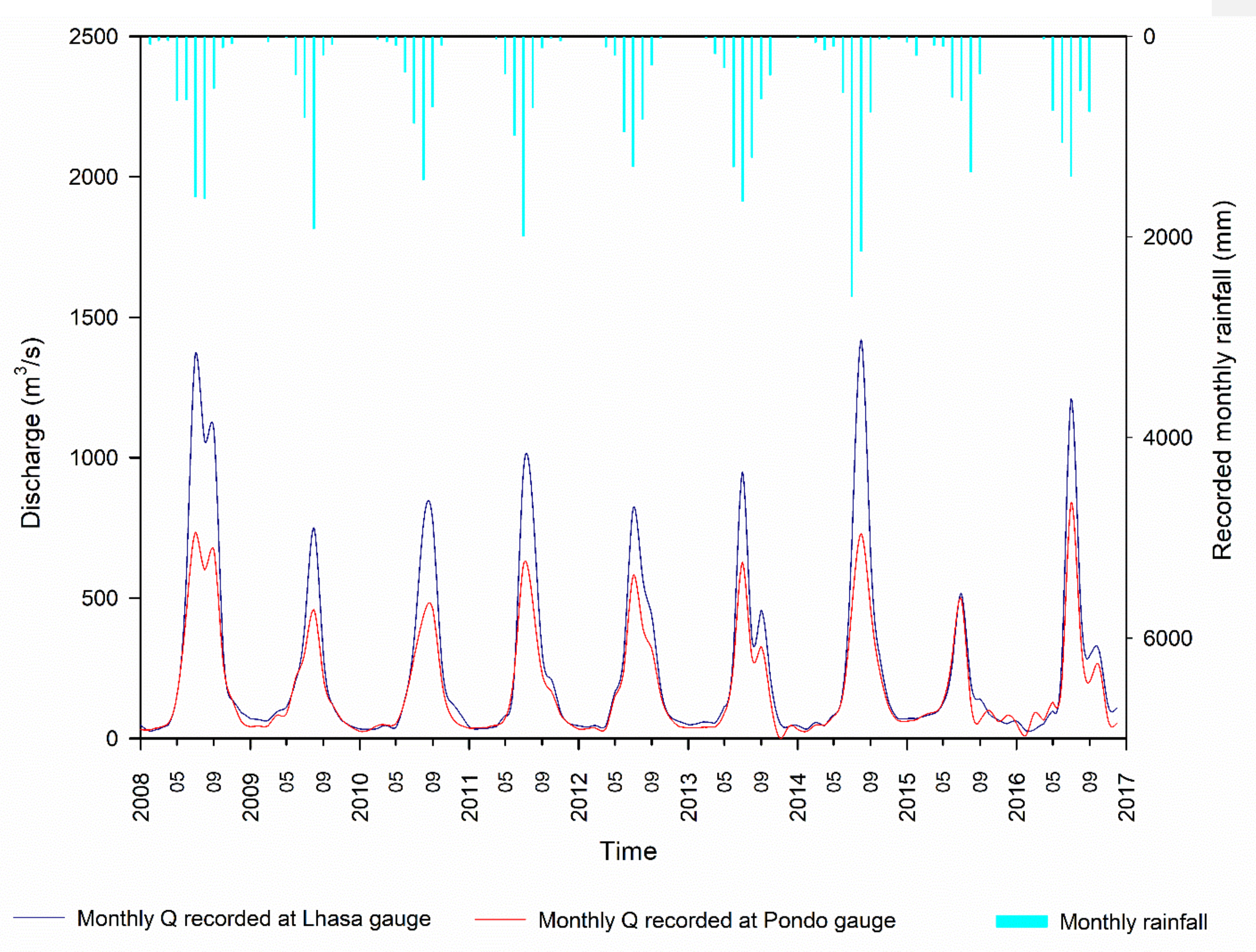
The hydrological regime of Lhasa River is a distinctive illustration of rainfall driven process. Figure 5 shows the rainfall dependency of Lhasa River discharge at two flow gauging stations, Pondo flow gauge near and Lhasa flow gauge downstream the reservoir chosen for the study. Lhasa streamflow gauge being located in the middle reach of the LRB receives the discharge generated from the whole catchment and is consequently peaking higher than the discharge accumulated at Pondo streamflow gauging station. Monthly streamflow obtained from average daily time series recorded at the hydrological stations increases with basin area [55]. However, for both the flow gauging stations, recorded river flow peaks during the time of summer months when high rainfall has occurred.
Mean monthly streamflow pattern in general is following the precipitation pattern, high in June–October with peaks in August and low in November–May [56] for both the flow gauging stations. With this background, the MK trend test and Sen’s slope has been used to identify the trend on seasonal (June–September) rainfall and streamflow for both the selected stations individually from years 2008–2016. Rainfall record for both the analyses is the same and is recorded at the Lhasa meteorological station.
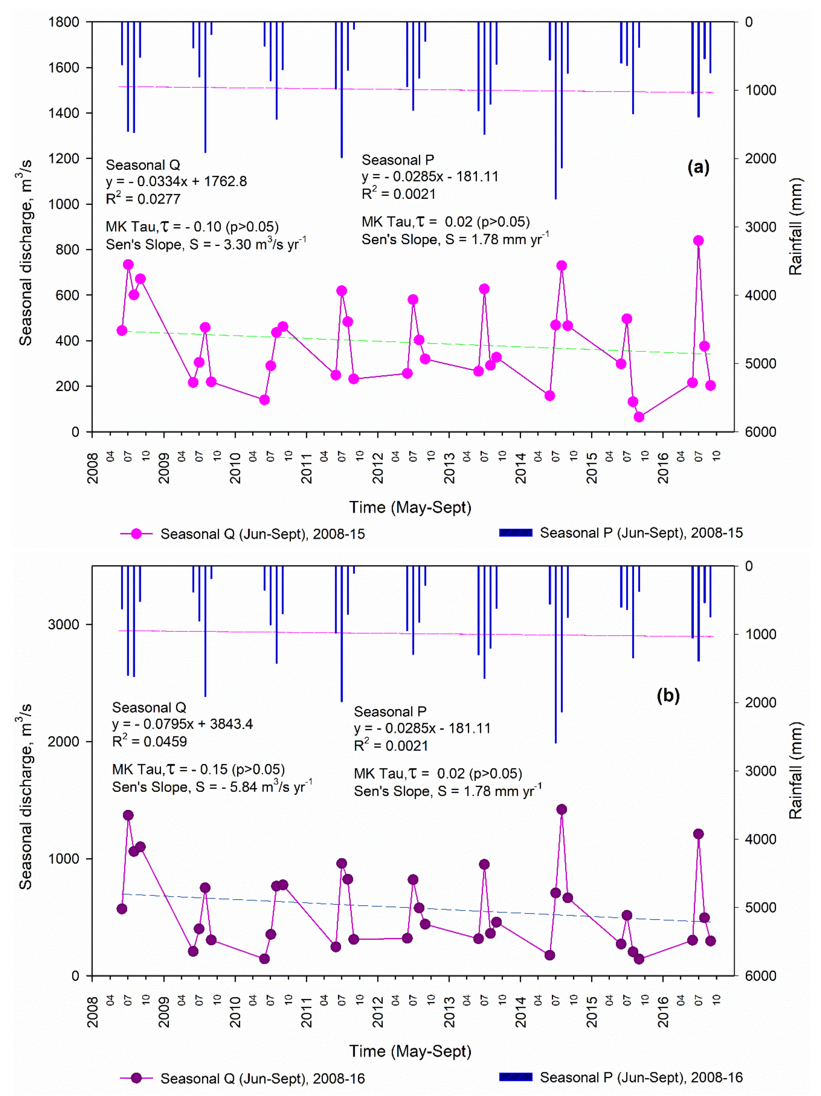
Figure 6a,b shows the MK trend on rainfall and streamflow for the Pondo and Lhasa flow gauging stations, respectively. The current study has revealed a non-significant (p > 0.05) increasing trend (positive MK Tau value) in the seasonal rainfall by 1.78 mm yr−1 (values for MK Tau and Sen’s slope are shown in Figure 6a,b). This is supported by [55] who have shown an increase in LRB rainfall using MK trend and Sen’s slope. However, their study has revealed a significant increase in rainfall. Here it is important to note that they have taken a long time span of monthly rainfall data for trend analysis, which affects the significance of the trend.
For the streamflow, the MK trend on the study time span has shown a non-significant decrease (negative values) for both the selected flow gauging stations (MK Tau and Sen’s slope values are shown in the Figure 6a,b). This again conforms to the findings of [55] where a non-significant decrease in the long-term streamflow recorded at two flow gauging stations, one of which is Lhasa flow gauge, has been reported for LRB. We see that the recorded seasonal discharge has decreased by greater magnitude (5.84 m3 s−1 yr−1) at Lhasa flow gauge. This again corresponds to the results of [55].

3.2. Lhasa River Flow Calibration, Validation and Parameter Sensitivity Analysis by SWAT

3.2.1. Streamflow Calibration, Validation and Parameter Sensitivity at Pondo Flow Gauge near the Selected Reservoir

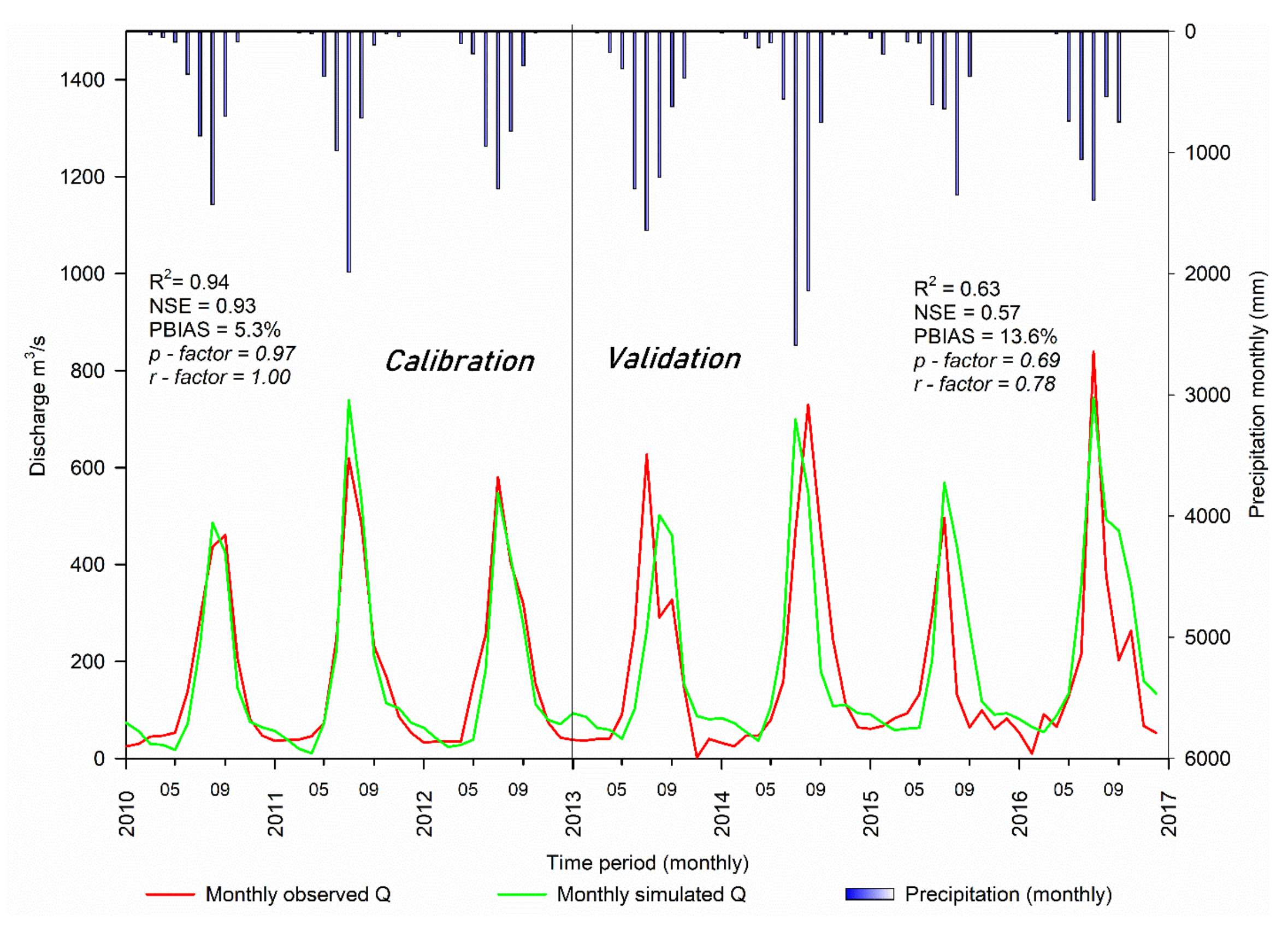
The performance of SWAT model is displayed as Figure 7 where the model has performed very well in calibrating the streamflow for the years pre-reservoir, functioning with high values of R2 and NSE and a small bias of 5.3% from the observed discharge at the flow gauging stations. The 95PPU plot envelopes the 97% of the simulated and observed values with a very close correspondence between the values. The values of P-factor and R-factor are definitely in agreement with what other researchers, e.g., Abbaspour (2015), recommended, i.e., p > 0.7 and r < 1.5. The calibrated parameters with their adjusted ranges, optimized values and rankings are presented as Table 3.
However, during the validation, which includes the reservoir functioning years, the performance of the model has decreased but still is within an acceptable range with R2 and NSE values greater than 0.5 and PBIAS less than 25%. The 95PPU envelope encloses 60% of the observed and simulated values, which is appreciably well extended. For flow, a practical value of 0.6–0.8 for the p-factor and a value around 1 for the r-factor are suggested [56]. We see that in trying to capture the peak events of river discharge, the model has fallen short for majority of the times, and on the contrary, low flows for dry season are frequently overestimated.

3.2.2. Streamflow Calibration, Validation and Parameter Sensitivity at Downstream Lhasa Flow Gauge

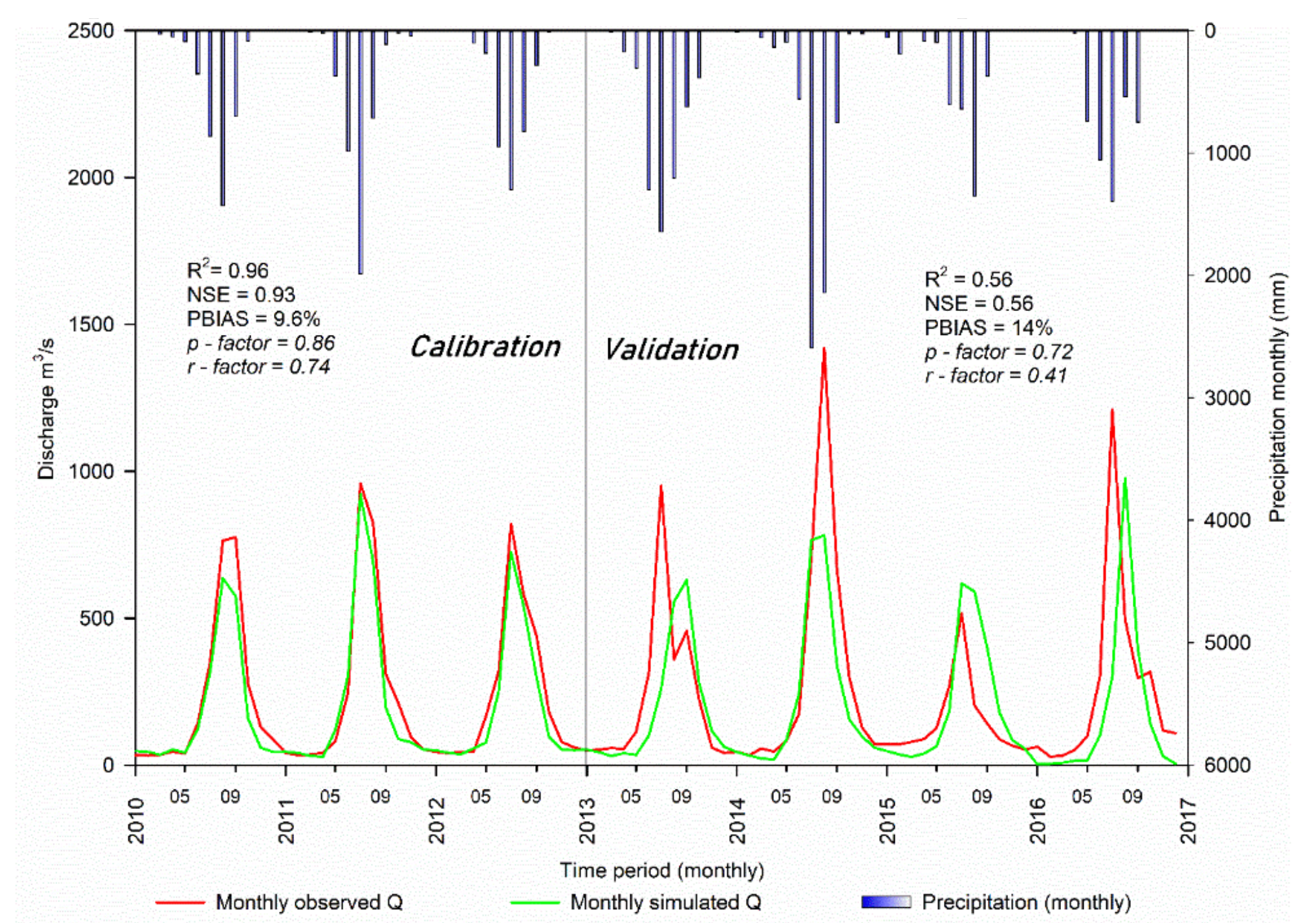
The model has been run to simulate monthly river discharge at the selected downstream Lhasa flow gauging station located near the LRB outlet. The model has produced a very closely conforming curve for monthly river flow (Figure 8) with R2 and NSE values of 0.96 and 0.93, respectively. The model has shown a very good performance while calibrating the monthly discharge for Lhasa River where it has slightly underestimated the high peak events with a PBIAS of 9.6%. The 95PPU band is enclosing 86% of the simulated and observed values with a p-factor of 0.86 and r-factor of 0.74 (Figure 8). The calibrated parameters with their fitted values and ranks are presented as Table 4.
For the validation years, the model has performed satisfactorily with R2 and NSE values of 0.56 for the correspondence of simulated discharge with the observed discharge (Figure 8). Many SWAT studies considered the model is reliable if the reported validation statistics are 0.5 or above (such as R2 > 0.5, NSE > 0.5) at the basin’s outlet [57]. However, the simulated values are biased with 14% underestimation from the observed values; so far, the model has performed well while simulating the river discharge. The 95PPU plot has been produced with 72% of values being enveloped in it.

3.3. ArcSWAT Depiction of Change in River Flow Pre and Post Reservoir Operation

3.3.1. Change in Streamflow Upstream the Selected Reservoir

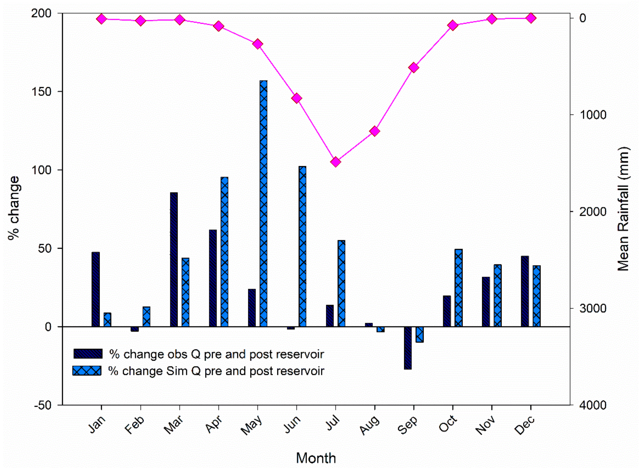
The observed and simulated river discharge for Pondo flow gauge has been analyzed for the percentage change as a consequence of reservoir operation in LRB. Figure 9 represents the behavior of change in river flow pre and post reservoir as revealed by the observed and model simulated discharge from 2010–2012 and 2013–2016, respectively. A substatntial increase in the dry season (November–May) observed river discharge at Pondo flow gauge has resulted, whereas, the wet season (June–October) undergoes either a decrease or a slight percent increase in the regulated observed discharge as a probable consequence of reservoir operation.
Regulated streamflow from reservoirs to downstream areas aids in moderating flood peaks and volumes and increasing base flow in dry season [58]. For model simulated streamflow, the model has shown a far more increase in the streamflow with progressively increasing rainfall events during the wet season under reservoir functioning. For the dry season, with decreasing rainfall the model has shown a better representation of increased streamflow obtained during the low rainfall months as the water stored during rainfall receiving summer months is available for use in winter dry months.

3.3.2. Change in Streamflow Downstream Selected Reservoir

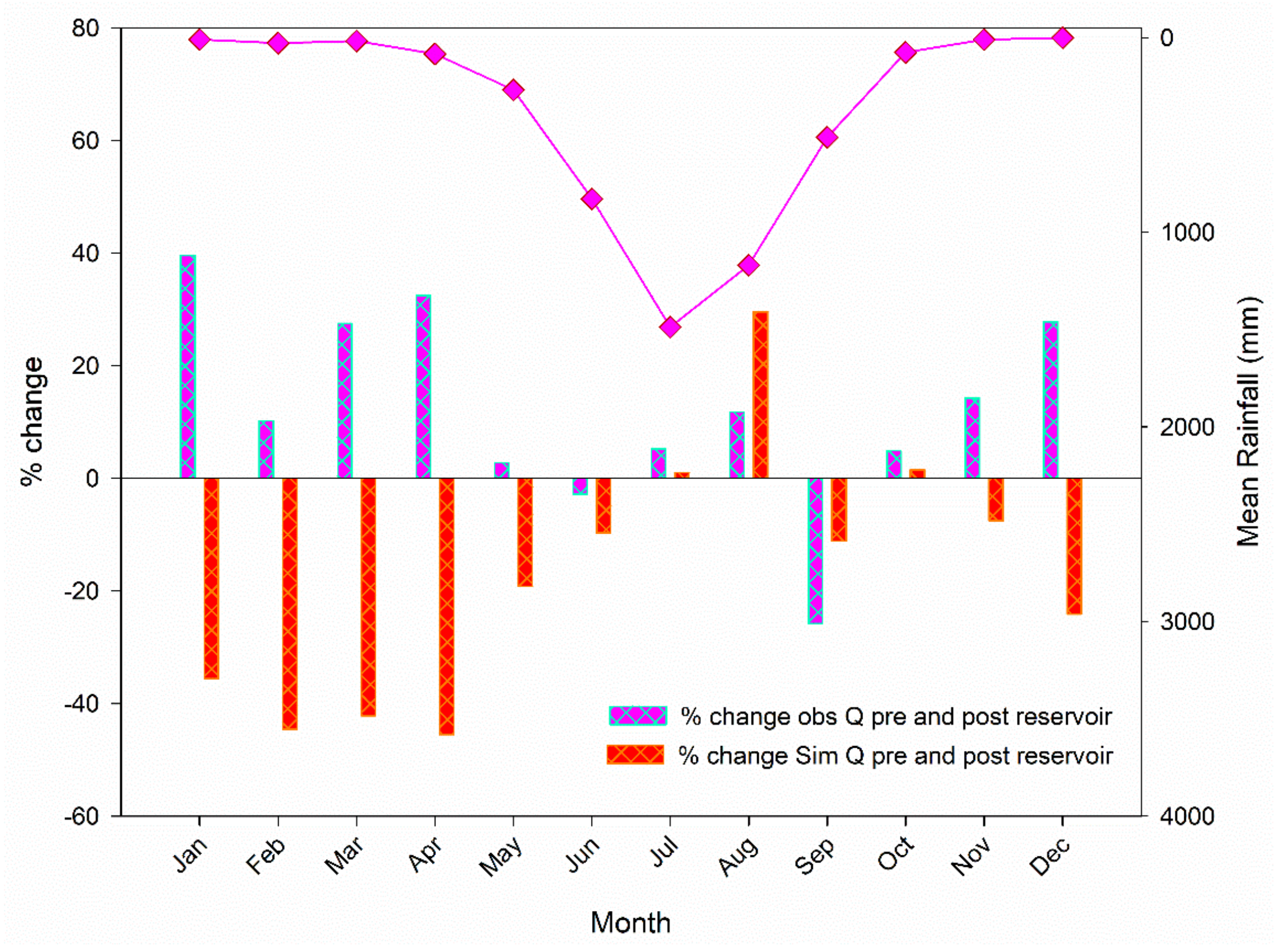
The regulated observed river flow at downstream Lhasa station shows a similar behavior of increased dry season (November–May) discharge and a decreased wet season (June–October) discharge, the evident outcome of reservoir functioning on the streamflow of Lhasa River. However, the percent change, whether increase or decrease, is comparatively smaller than the change observed at the upstream flow gauge. The simulated river discharge for the Lhasa flow gauge has shown a deviation from the observed river discharge for both the wet and dry seasons (Figure 10). According to [30], the further downstream the station is located, the greater the departure between the two simulations.

3.4. Inter-Relationship between Water Level and Inflow of Pangduo Reservoir and ArcSWAT Streamflow Simulation (Up and Downstream)

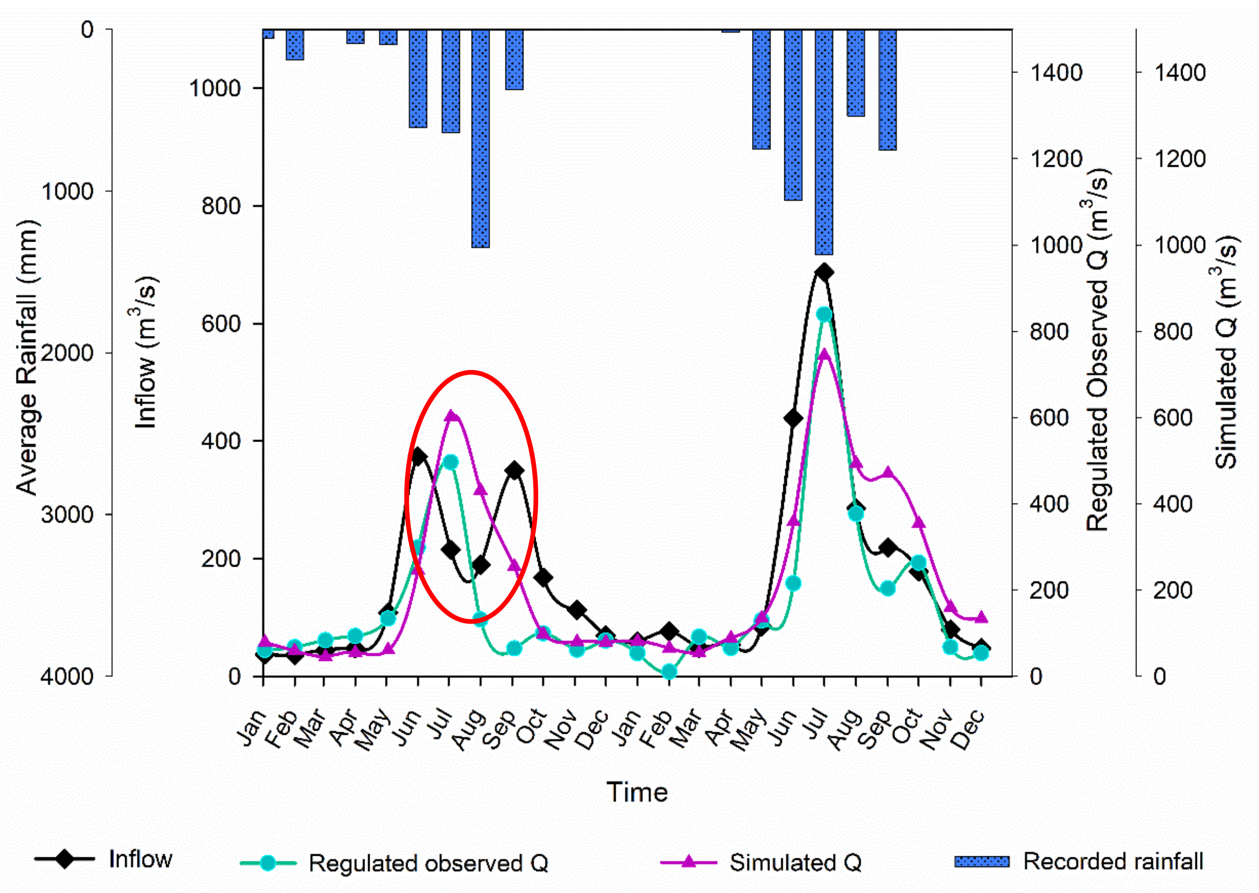
To further understand the hydrological phenomena of Lhasa River under the influence of reservoir operation, the available data for reservoir water level for the year 2015 has been used to evaluate the performance of ArcSWAT simulation under reservoir operation (Figure 11). We see that the reservoir water level agrees with the rainfall events; however, the river discharge decreases as the water is stored, filling up the reservoir.
At the selected flow gauges, the simulated river flow exhibits a similar characteristic as the observed discharge. i.e., lowering of peaks during the high rainfall month of August, revealing that the summer flow is being donated for use in the low rainfall winter months. We see that the simulated flow is overestimated; however, the model has performed comparatively well for Pondo station, which is located near the reservoir, as it is prone to a relatively lesser impact from the reservoir compared to the farther downstream Lhasa gauging station for which the simulated discharge fluctuates wider from the observed discharge. Here, it is important to mention that 2015 was a year with a very low recorded rainfall compared to other years from 2008–2016. This lower rainfall has resulted in an exceptionally lower river discharge for the same year. The reservoir water level during the high rainfall months of July and August is found to be lower than the dead water level of 4066 m (Table 1). The water level in the reservoir is again replenished to normal water level by the months of September and October. This reveals an unusual hydrological situation in the LRB during the reference year, which can be possibly a data record error. This provides a basis for the significance of the model simulated results presented above, since with such lower recorded rainfall, the model still managed to produce some appreciable results.
The SWAT simulation displayed a better representation for the upstream Pondo flow gauge; thus, it was used to develop a relationship with the inflow of reservoir, which was available for the years 2015–2016 (Figure 12). The inflow data being available only for two years, there were some missing data for 15 July–15 August (highlighted in Figure 12), which is the time for high rainfall and river flow peak. We see a relatively lower observed river discharge also for the same time.
River discharge can be used as reservoir outflow in case of unavailability of reservoir outflow record. The model-simulated river discharge shows a fairly close correspondence with the inflow to reservoir and observed river discharge as it is used in place of reservoir outflow.

4. Discussion

4.1. Hydrological Institution of Lhasa River Basin and the Resevoir Operation

Cuo et al. 2019 [55] has shown that LRB streamflow modifies in correspondence with the monthly precipitation, peaking high in wet months and vice versa. Figure 6a,b represent that precipitation being the controlling factor in Lhasa River discharge, the increased rainfall during the study time is resulting in a monthly discharge which is decreasing over time. On the other hand, in Figure 4, the annual river discharge recorded at both the stations is increasing by the end years except for 2015, with the lowest recorded discharge. In the past decades, the quantity of streamflow has improved on a global scale [59] which might have stemmed from the increased precipitation, for the increased precipitation has become more apparent in Southern China, US, and countries in Europe and South America [59,60,61,62,63]. However, several studies show increased precipitation merely is not enough to explain streamflow variability in the watersheds and even some inverse trends have been observed in some watersheds [64,65]. The influence of climate change on streamflow regimes varies with geographical location and watershed characteristics [66,67].
This brings us to the deduction that besides climatic factors, other factors are also operating in determining the hydrological phenomena of LRB. As per our study, the major proportion of river discharge produced during wet warm season is shifted to the cold dry season of lower rainfall, thus causing a decrease in monthly river discharge. The reservoir operations and water abstraction unsurprisingly headed to changes in the natural flow regime and decrease of flow in the downstream river [68]. Human activities exclusively damming have been frequently documented as the element causing streamflow regime variation. Since the preceding four decades, the influence of dams and its flow regulations have produced much debate; it has instigated ecological harms but also enhanced water security, flood control, and power generation [69,70].

4.2. About SWAT Simulation of Streamflow at Selected Flow Gauge Sites under Reservoir Influence

Using the SWAT model, we evaluated streamflow simulations in the LRB based on reservoir operation scheme. Reservoir operations have both direct and indirect effects on streamflow. Water release from reservoirs directly affects the magnitude and variability of streamflow in downstream reaches. Dam and water diversion operations determine the amount and timing of water discharge to downstream river channels. As a result, reservoir operations may either lessen flood peaks in wet seasons or increase streamflow in dry years, in agreement with minimum instream flow policies [71]. Similar impact of reservoir has been observed for LRB where the discharge has been experiencing a reduction particularly during the high rainfall months generating the high peaks during the summer months. We have assessed the river discharge pattern of LRB at two flow gauge sites in order to develop a better understanding of the hydrological behavior of Lhasa River under reservoir influence. For this purpose, SWAT modelling achieved better performance criteria for the upstream flow gauging station. However for Pondo flow gauging station, SWAT model has produced an over-estimation for the dry season and an under-estimation for the wet season (Figure 9). Tian et al. 2020 [72] has also reported an under-estimation of Lhasa River discharge simulation by SWAT model. This phenomenon has been further reported by SWAT model reliability assessments conducted for the PoKo [73], Cong [74] and Nam Kim [75] watersheds in Vietnam where the model performed well for overall streamflow simulation but did not match some peaks accurately. For Lhasa station, the deviation has increased being lying downstream the reservoir. Other possible reason may be operation of Zhikong reservoir downstream (Figure 1) the Pangduo reservoir causing a further decrease in the Lhasa River discharge at the basin outlet. In addition to reservoir operations, cropland irrigation also affects watershed hydrology. Water withdrawal for irrigation has been widely adopted to increase crop production in arid and semi-arid regions. Water redistribution through irrigation enhances water and energy fluxes between soils and the atmosphere [76] and results in elevated water loss through evapotranspiration [77,78,79] and depletion of water resources [80] in different regions of the world. April–May is a sowing, seedling, and tillering season in the Yarlung Tsangbo valley [81,82,83]. In LRB, with runoff in April and May accounting for 1.7% and 3.5% of the annual total in LRB, respectively where only 0.6–13.7% of the annual precipitation occurs in April and May, irrigation plays a critical role in April–May due to a lack of precipitation which is also supported by [81,82,83]. Further, in the Yarlung Tsangbo valley catchments, water used for irrigation comes solely from surface water stored by reservoirs [84]. Sridhar et al. [85] has reported that the dams result in a decreased streamflow feasibly for irrigation water conveyance. Scenarios with irrigation practices demonstrat higher water losses through evapotranspiration (ET) and match benchmark data better than the scenario that only consider reservoir operations [86]. In addition, multiple hydrological processes, such as vertical flow in surface or subsurface waters, water routing, evaporation, precipitation, and microclimate, are also responsive to reservoir operations [87]. Thus, for a better model representation of hydrological phenomena of LRB, it is recommended to carry out scenario based investigations. Also, reservoir operation data unavailability and discrepancy is a hurdle in the present reservoir operation based study. Regarding the performance criteria of SWAT modelling (R2, NSE, PBIAS), it is worth noting that these statistical metrics are calculated based on a limited set of hydrological variables (e.g., streamflow) and cannot guarantee that other hydrological processes are well represented [88]. Thus, the current study can be beneficial for decisions regarding the reservoir operation influences on streamflow spatially along the watershed in other similar settings around the globe.

4.3. Limitations of the Study

For the present study, the major limitation has been data availability and its quality. LRB is considered a data sensitive area of Qinghai-Tibetan region. The data sharing and recording on hydrological resources is a major concern in the study area. The study utilized the very short term available data on reservoir water level and inflow. To assess the real situation of reservoir functioning, its influence on the downstream areas and water allocation for multiple uses, long term data availability needs to be ensured.
The current study has applied built-in SWAT model reservoir module as a first step to assess the water resource and management phenomena in LRB. Further analyses involving the associated vital influencing factors on the hydrological process are critically important for a better understanding of water resource condition in future.

5. Conclusions

The current study has emphasized the influence of establishment of Pangduo reservoir on the hydrological situation of Lhasa River. The study reveals that the streamflow of LRB, being strongly dependent on the rainfall, is prone to the Pangduo reservoir functioning and is experiencing a decrease across the study time span during the high discharge wet warm months both at Pondo and Lhasa hydrometric stations. However, the magnitude of decrease is found to be more on the discharge accumulated downstream at Lhasa flow gauge station being more exposed to the effect of reservoir storage of streamflow. The total discharge recorded at Lhasa station is higher as it is received from the entire basin. Apart from reservoir functioning, other processes like irrigation practices and ground water withdrawal may be some very vital factors for water volume reduction in the Lhasa River and needs to be addressed for further understanding of the hydrological scenario of LRB.
The current modelling presentation shows the expediency of SWAT in determining the hydrological phenomena of LRB under the reservoir influence at Pondo and Lhasa hydrometric stations and reveals a better simulation of streamflow at upstream Pondo flow gauge, considering only the reservoir functioning and not the integral processes of multi-purpose water abstractions for other management and human activities. The performance of the model is expected to improve by considering the closely associated hydrological processes affecting the streamflow in LRB. The simulated discharge for Pondo flow gauge is in fairly close correspondence with the reservoir operation procedures such as water level and inflow. This concludes that the present study can benefit local authorities for decision making regarding the water distribution under reservoir influence along various parts of the LRB.

Author Contributions

This research is carried out in collaboration with all authors. Conceptualization, M.Y., T.H.; methodology, M.Y.; software, M.Y., S.A.H.; validation, M.Y., S.A.H.; formal analysis, M.Y.; data curation, T.H.; writing—original draft preparation, M.Y.; writing—review and editing, T.H.; supervision, T.H.; project administration, T.H.; funding acquisition, T.H. All authors have read and agreed to the published version of the manuscript.

Funding

This study has been supported by the National Natural Science Foundation of China (Grant No. 91647204).

Acknowledgments

We thank three anonymous reviewers and editors for constructive suggestions and comments.

Conflicts of Interest

The authors declare no conflict of interest.

References

  1. Naiman, R.J.; Decamps, H.; Pollock, M. The Role of Riparian Corridors in Maintaining Regional Biodiversity. Ecol. Appl. 1993, 3, 209–212. [Google Scholar] [CrossRef]
  2. Chen, X.; Yan, Y.; Fu, R.; Dou, X.; Zhang, E. Sediment transport from the Yangtze River, China, into the sea over the post-three gorge dam period: A discussion. Quat. Int. 2008, 186, 55–64. [Google Scholar] [CrossRef]
  3. Rosegrant, M.W.; Cai, X.; Cline, S.A. World Water and Food to 2025: Dealing with Scarcity; International Food Policy Research Institute: Washington, DC, USA, 2002. [Google Scholar]
  4. Gleick, P.H. China Dams, the World’s Water; Island Press: Washington, DC, USA, 2012. [Google Scholar]
  5. REN21. Renewables 2014: Global Status Report (Paris: REN21 Secretariat); Technical Report; REN21: Paris, France, 2014; ISBN 978-3-9815934-2-6. [Google Scholar]
  6. Spänhoff, B. Current status and future prospects of hydropower in Saxony (Germany) compared to trends in Germany, the European Union and the World. Renew. Sustain. Energy Rev. 2014, 30, 518–525. [Google Scholar] [CrossRef]
  7. Yang, J.; Liu, Q.; Li, X.; Cui, X. Overview of Wind Power in China: Status and Future. Sustainability 2017, 9, 1454. [Google Scholar] [CrossRef] [Green Version]
  8. Frey, S.K.; Topp, E.; Ball, B.R.; Edwards, M.; Gottschall, N.; Sunohara, M.; Zoski, E.; Lapen, D.R. Tile Drainage Management Influences on Surface-Water and Groundwater Quality following Liquid Manure Application. J. Environ. Qual. 2013, 42, 881–892. [Google Scholar] [CrossRef]
  9. Condon, L.E.; Maxwell, R.M. Feedbacks between managed irrigation and water availability: Diagnosing temporal and spatial patterns using an integrated hydrologic model. Water Resour. Res. 2014, 50, 2600–2616. [Google Scholar] [CrossRef]
  10. De Schepper, G.; Therrien, R.; Refsgaard, J.C.; Hansen, A.L. Simulating coupled surface and subsurface water flow in a tile-drained agricultural catchment. J. Hydrol. 2015, 521, 374–388. [Google Scholar] [CrossRef]
  11. Wu, K.; Xu, Y.J. Evaluation of the applicability of the SWAT model for coastal watersheds in southeastern Louisiana1. JAWRA J. Am. Water Resour. Assoc. 2006, 42, 1247–1260. [Google Scholar] [CrossRef]
  12. Viviroli, D.; Zappa, M.; Gurtz, J.; Weingartner, R. An introduction to the hydrological modelling system PREVAH and its pre- and post-processing-tools. Environ. Model. Softw. 2009, 24, 1209–1222. [Google Scholar] [CrossRef]
  13. Zhu, X.; Zhang, C.; Qi, W.; Cai, W.; Zhao, X.; Wang, X. Multiple Climate Change Scenarios and Runoff Response in Biliu River. Water 2018, 10, 126. [Google Scholar] [CrossRef] [Green Version]
  14. Bhuyan, S.J.; Koelliker, J.K.; Marzen, L.J.; Harrington, J.A. An integrated approach for water quality assessment of a Kansas watershed. Environ. Model. Softw. 2003, 18, 473–484. [Google Scholar] [CrossRef]
  15. Tahir, A.A.; Hakeem, S.A.; Hu, T.; Hayat, H.; Yasir, M. Simulation of snowmelt-runoff under climate change scenarios in a data-scarce mountain environment. Int. J. Digit. Earth 2017, 12, 910–930. [Google Scholar] [CrossRef]
  16. Arnold, J.G.; Srinivasan, R.; Muttiah, R.S.; Williams, J.R. Large area hydrologic modeling and assessment Part I: Model development 1. JAWRA J. Am. Water Resour. Assoc. 1998, 34, 73–89. [Google Scholar] [CrossRef]
  17. Bärlund, I.; Kirkkala, T.; Malve, O.; Kämäri, J. Assessing SWAT model performance in the evaluation of management actions for the implementation of the Water Framework Directive in a Finnish catchment. Environ. Model. Softw. 2007, 22, 719–724. [Google Scholar] [CrossRef]
  18. Kaur, R.; Srivastava, R.; Betne, R.; Mishra, K.; Dutta, D. Integration of linear programming and a watershed-scale hydrologic model for proposing an optimized land-use plan and assessing its impact on soil conservation—A case study of the Nagwan watershed in the Hazaribagh district of Jharkhand, India. Int. J. Geogr. Inf. Sci. 2004, 18, 73–98. [Google Scholar] [CrossRef]
  19. Sun, H.; Cornish, P.S. A catchment-based approach to recharge estimation in the Liverpool Plains, NSW, Australia. Aust. J. Agric. Res. 2006, 57, 309–320. [Google Scholar] [CrossRef]
  20. Schuol, J.; Abbaspour, K.C. Calibration and uncertainty issues of a hydrological model (SWAT) applied to West Africa. Adv. Geosci. 2006, 9, 137–143. [Google Scholar] [CrossRef] [Green Version]
  21. Hao, F.-H.; Zhang, X.-S.; Yang, Z.-F. A distributed non-point source pollution model: Calibration and validation in the Yellow River Basin. J. Environ. Sci. (China) 2004, 16, 646–650. [Google Scholar]
  22. Coerver, H.M.; Rutten, M.M.; Van de Giesen, N.C. Deduction of reservoir operating rules for application in global hydrological models. Hydrol. Earth Syst. Sci. 2018, 22, 831. [Google Scholar] [CrossRef] [Green Version]
  23. Lu, X.X. Water discharge and sediment flux changes over the past decades in the Lower Mekong River: Possible impacts of the Chinese Dams. Hydrol. Earth Syst. Sci. 2006, 10, 181–195. [Google Scholar] [CrossRef] [Green Version]
  24. Reeves, J.; Chen, J.; Wang, X.L.L.; Lund, R.; Lu, Q. nA review and comparison of change point detection techniques for climate data. J. Appl. Meteorol. Climatol. 2007, 46, 900–915. [Google Scholar] [CrossRef]
  25. Cloern, J.E.; Abreu, P.C.; Carstensen, J.; Chauvaud, L.; Elmgren, R.; Grall, J.; Greening, H.; Johansson, J.O.R.; Kahru, M.; Sherwood, E.T.; et al. Human activities andclimate variability drive fast-paced change across the world’ sestuarine-coastal ecosystems. Glob. Chang. Biol. 2016, 22, 513–529. [Google Scholar] [CrossRef] [PubMed]
  26. Wu, H.S.; Liu, D.F.; Chang, J.X.; Zhang, H.X.; Huang, Q. Impacts of climate change and human activities on run off in Weihe Basin based on Budykohypothesis. IOP Conf. Ser. Earth Env. Sci. 2017, 82, 012063. [Google Scholar] [CrossRef] [Green Version]
  27. Zhang, A.J.; Zheng, C.M.; Wang, S.; Yao, Y.Y. Analysis of stream flow variations in the Heihe River Basin, northwest China: Trends, abruptchanges, driving factors and ecological influences. J. Hydrol. 2015, 3, 106–124. [Google Scholar] [CrossRef]
  28. Koch, F.; Prasch, M.; Bach, H.; Mauser, W.; Appel, F.; Weber, M. How Will Hydroelectric Power Generation Develop under Climate Change Scenarios? A Case Study in the Upper Danube Basin. Energies 2011, 4, 1508. [Google Scholar] [CrossRef]
  29. Stojković, M.; Ilić, A.; Prohaska, S.; Plavšić, J. Multi-temporal analysis of mean annual and seasonal streamflowtrends, including periodicity and multiplenonlinear regression. Water Resour. Manag. 2014, 28, 4319–4335. [Google Scholar] [CrossRef]
  30. Canuto, N.; Ramos, T.B.; Oliveira, A.R.; Simionesei, L.; Basso, M.; Neves, R. Influence of reservoir management on Guadiana streamflow regime. J. Hydrol. Reg. Stud. 2019, 25, 100628. [Google Scholar] [CrossRef]
  31. Wu, J.; Chen, X.; Yu, Z.; Yao, H.; Li, W.; Zhang, D. Assessing the impact of human regulations on hydrological drought development and recovery based on a ‘simulated-observed’ comparison of the SWAT model. J. Hydrol. 2019, 577, 123990. [Google Scholar] [CrossRef]
  32. Tu, X.; Wu, H.; Singh, V.P.; Chen, X.; Lin, K.; Xie, Y. Multivariate design of socioeconomic drought and impact of water reservoirs. J. Hydrol. 2018, 566, 192. [Google Scholar] [CrossRef]
  33. Zhang, Q. Evaluation of ecological instream flow using multiple ecological indicators with consideration of hydrological alterations. J. Hydrol. 2015, 529, 711–722. [Google Scholar] [CrossRef]
  34. Zhang, Y.; Wang, C.; Bai, W.; Zhaofeng, W.; Yanli, T.; Dor, G.Y. Alpine wetlands in the Lhasa River Basin, China. J. Geogr. Sci. 2010, 20, 375–388. [Google Scholar] [CrossRef]
  35. Kendall, M.; Gibbons, J.D. Rank Correlation Methods. Charles Griffin Book Series, 5th ed.; Oxford University Press: Oxford, UK, 1990; ISBN 978-0195208375. [Google Scholar]
  36. Arnold, J.G.; Allen, P.M.; Bernhardt, G. A comprehensive surface-groundwater flow model. J. Hydrol. 1993, 142, 47–69. [Google Scholar] [CrossRef]
  37. Jha, M.K. Evaluating Hydrologic Response of an Agricultural Watershed for Watershed Analysis. Water 2011, 3, 604–617. [Google Scholar] [CrossRef]
  38. Kannan, N.; White, S.M.; Worrall, F.; Whelan, M.J. Hydrological modelling of a small catchment using SWAT-2000–Ensuring correct flow partitioning for contaminant modelling. J. Hydrol. 2007, 334, 64–72. [Google Scholar] [CrossRef]
  39. Gassman, P.W.; Reyes, M.R.; Green, C.H.; Arnold, J.G. The Soil and Water Assessment Tool: Historical Development, Applications, and Future Research Directions. Trans. Asabe 2007, 50, 1211–1250. [Google Scholar] [CrossRef] [Green Version]
  40. Douglas-Mankin, K.R.; Srinivasan, R.; Arnold, J.G. Soil and Water Assessment Tool (SWAT) Model: Current Developments and Applications. Trans. Asabe 2010, 53, 1423–1431. [Google Scholar] [CrossRef]
  41. Tuppad, P.; Douglas-Mankin, K.R.; Lee, T.; Srinivasan, R.; Arnold, J.G. Soil and Water Assessment Tool (SWAT) Hydrologic/Water Quality Model: Extended Capability and Wider Adoption. Trans. ASABE 2011, 54, 1677–1684. [Google Scholar] [CrossRef]
  42. Van Griensven, A.; Ndomba, P.; Yalew, S.; Kilonzo, F. Critical review of SWAT applications in the upper Nile basin countries. Hydrol. Earth Syst. Sci. 2012, 16, 3371–3381. [Google Scholar] [CrossRef] [Green Version]
  43. Gassman, P.W.; Sadeghi, A.M.; Srinivasan, R. Applications of the SWAT Model Special Section: Overview and Insights. J. Environ. Qual. 2014, 43, 1–8. [Google Scholar] [CrossRef]
  44. Krysanova, V.; White, M. Advances in water resources assessment with SWAT—an overview. Hydrol. Sci. J. 2015, 60, 771–783. [Google Scholar] [CrossRef] [Green Version]
  45. Neitsch, S.L.; Arnold, J.G.; Kiniry, J.R.; Williams, J.R. Soil and Water Assessment Tool Theoretical Documentation–Version 2009; (TR-406); Texas Water Resources Institute: College Station, TX, USA, 2011. [Google Scholar]
  46. Khoi, D.N.; Thom, V.T. Parameter uncertainty analysis for simulating streamflow in a river catchment of Vietnam. Glob. Ecol. Conserv. 2015, 4, 538–548. [Google Scholar] [CrossRef] [Green Version]
  47. Abbaspour, K.C.; Yang, J.; Maximov, I.; Siber, R.B.K.; Mieleitner, J.; Zobrist, J.; Srinivasan, R. Modelling hydrology and water quality in the pre-alpine/alpine Thur watershed using SWAT. J. Hydrol. 2007, 333, 413–430. [Google Scholar] [CrossRef]
  48. Zhao, F.; Wu, Y.; Qiu, L.; Sun, Y.; Sun, L.; Li, Q.; Niu, J.; Wang, G. Parameter Uncertainty Analysis of the SWAT Model in a Mountain-Loess Transitional Watershed on the Chinese Loess Plateau. Water 2018, 10, 690. [Google Scholar] [CrossRef] [Green Version]
  49. Santhi, C.; Arnold, J.G.; Williams, J.R.; Dugas, W.A.; Srinivasan, R.; Hauck, L.M. Validation of the SWAT model on a large basin with point and nonpoint sources 1. JAWRA J. Am. Water Resour. Assoc. 2001, 37, 1169–1188. [Google Scholar] [CrossRef]
  50. Mihon, D.; Bacu, V.; Denisa, R.; Teodor, S.; Karim, A.; Elham, R.; Dorian, G. Grid Based Hydrologic Model Calibration and Execution. In Advances in Intelligent Control Systems and Computer Science; Dumitrache, L., Ed.; Springer: Berlin/Heidelberg, Germany, 2013; pp. 279–293. [Google Scholar]
  51. Nash, J.E.; Sutcliffe, J.V. River flow forecasting through conceptual models part I—A discussion of principles. J. Hydrol. 1970, 10, 282–290. [Google Scholar] [CrossRef]
  52. Moriasi, D.N.; Arnold, J.G.; Van Liew, M.W.; Bingner, R.L.; Harmel, R.D.; Veith, T.L. Model Evaluation Guidelines for Systematic Quantification of Accuracy in Watershed Simulations. Trans. Asabe 2007, 50, 885–900. [Google Scholar] [CrossRef]
  53. Gupta Hoshin, V.; Sorooshian, S.; Yapo Patrice, O. Status of Automatic Calibration for Hydrologic Models: Comparison with Multilevel Expert Calibration. J. Hydrol. Eng. 1999, 4, 135–143. [Google Scholar] [CrossRef]
  54. Searcy, J.K. Flow-Duration Curves: Manual of Hydrology: Part 2: Low-Flow Techniques; US Government Printing Office: Washington, DC, USA, 1959.
  55. Cuo, L.; Li, N.; Liu, Z.; Ding, J.; Liang, L.; Zhang, Y.; Gong, T. Warming and human activities induced changes in the Yarlung Tsangpo basin of the Tibetan plateau and their influences on streamflow. J. Hydrol. Reg. Stud. 2019, 25, 100625. [Google Scholar] [CrossRef]
  56. Faramarzi, M.; Abbaspour, K.C.; Adamowicz, W.L.; Lu, W.; Fennell, J.; Zehnder, A.J.B.; Goss, G.G. Uncertainty based assessment of dynamic freshwater scarcity in semi-arid watersheds of Alberta, Canada. J. Hydrol. Reg. Stud. 2017, 9, 48–68. [Google Scholar] [CrossRef]
  57. Tan, M.L.; Gassman, P.W.; Srinivasan, R.; Arnold, J.G.; Yang, X. A Review of SWAT Studies in Southeast Asia: Applications, Challenges and Future Directions. Water 2019, 11, 914. [Google Scholar] [CrossRef] [Green Version]
  58. Batalla, R.J. Reservoir-induced hydrological changes in the Ebro River basin (NE Spain). J. Hydrol. 2004, 290, 117–136. [Google Scholar] [CrossRef]
  59. Najjar, R.G.; Pyke, C.R.; Adams, M.B.; Breitburg, D.; Hershner, C.; Kemp, M.; Howarth, R.; Mulholland, R.; Paolisso, M.; Secor, D.; et al. Potential climate-change impacts on the Chesapeake Bay. Estuar. Coast. Shelf Sci. 2010, 86, 1–20. [Google Scholar] [CrossRef]
  60. Struyf, E.; Van Damme, S.; Meire, P. Possible effects of climate change on estuarine nutrient fluxes: A case study in the highly nutrified Schelde estuary (Belgium, the Netherlands). Estuar. Coast. Shelf Sci. 2004, 60, 649–661. [Google Scholar] [CrossRef] [Green Version]
  61. Tomer, M.D.; Schilling, K.E. A simple approach to distinguish land-use and climate-change effects on watershed hydrology. J. Hydrol. 2009, 376, 24–33. [Google Scholar] [CrossRef]
  62. Xu, K.; Milliman, J.D.; Xu, H. Temporal trend of precipitation and runoff in major Chinese Rivers since 1951. Glob. Planet. Chang. 2010, 73, 219–232. [Google Scholar] [CrossRef]
  63. Doyle, M.E.; Saurral, R.I.; Barros, V.R. Trends in the distributions of aggregated monthly precipitation over the La Plata Basin. Int. J. Climatol. 2012, 32, 2149–2162. [Google Scholar] [CrossRef]
  64. Kustu, M.D.; Fan, Y.; Rodell, M. Possible link between irrigation in the US High Plains and increased summer streamflow in the Midwest. Water Resour. Res. 2011, 47, W03522. [Google Scholar] [CrossRef]
  65. Fan, J.; Tian, F.; Yang, Y.H.; Han, S.; Qiu, G. Quantifying the magnitude of the impact of climate change and human activities on runoff decline in Mian River Basin, China. Water Sci. Technol. 2010, 62, 783–791. [Google Scholar] [CrossRef]
  66. Xu, C.Y.; Gong, L.B.; Jiang, T.; Chen, D.; Singh, V.P. Analysis of spatial distribution and temporal trend of reference evapotranspiration in Changjiang (Yangtze River) catchment. J. Hydrol. 2006, 327, 81–93. [Google Scholar] [CrossRef]
  67. Ye, X.C.; Zhang, Q.; Liu, J.; Li, X.; Xu, C.-Y. Distinguishing the relative impacts of climate change and human activities on variation of streamflow in the Poyang Lake catchment, China. J. Hydrol. 2013, 494, 83–95. [Google Scholar] [CrossRef]
  68. Li, S.; Xiong, L.H.; Dong, L.H.; Zhang, J. Effects of Three Gorges reservoir on the hydrological droughts at the downstream Yichang station during 2003–2011. Hydrol. Process. 2013, 27, 3981–3993. [Google Scholar] [CrossRef]
  69. Richter, B.D.; Thomas, G.A. Restoring environmental flows by modifying dam operations. Ecol. Soc. 2007, 12, 12. [Google Scholar] [CrossRef]
  70. Petts, G.E. Instream-flow science for sustainable river management. J. Am. Water Resour. Assoc. 2009, 45, 1071–1086. [Google Scholar] [CrossRef] [Green Version]
  71. Yoder, J.; Jonathan, A.; Jennifer, B.; Michael, C.; Joseph, K.; Stephen, J.; Shane, M.K.; McMillan, J.; Yang, Q. Benefit-Cost Analysis of Integrated Water Resource Management: Accounting for Interdependence in the Yakima Basin Integrated Plan. J. Am. Water Resour. Assoc. 2017, 53, 456. [Google Scholar] [CrossRef]
  72. Tian, P.; Lu, H.; Feng, W.; Guan, Y.; Xue, Y. Large decrease in streamflow and sediment load of Qinghai–Tibetan Plateau driven by future climate change: A case study in Lhasa River Basin. CATENA 2020, 187, 104340, ISSN 0341-8162. [Google Scholar] [CrossRef]
  73. Tram, V.Q.; Liem, N.D.; Loi, N.K. Assessing Water Availability in PoKo Catchment using SWAT model. Khon Kaen Agric. J. 2014, 42, 74–84. [Google Scholar]
  74. Anh, N.V.; Fukuda, S.; Hiramatsu, K.; Harada, M. Sensitivity-Based Calibration of the Soil and Water Assessment Tool for Hydrologic Cycle Simulation in the Cong Watershed, Vietnam. Water Env. Res. 2015, 87, 735–750. [Google Scholar] [CrossRef]
  75. Nguyen, H.Q.; Kappas, M. Modeling Surface Runoff and Evapotranspiration using SWAT and BEACH for a Tropical Watershed in North Vietnam, Compared to MODIS Products. Int. J. Adv. Remote Sens. Gis 2015, 4, 1367–1384. [Google Scholar] [CrossRef] [Green Version]
  76. Rost, S.; Gerten, D.; Bondeau, A.; Luncht, W.; Rohwer, J.; Schaphoff, S. Agricultural green and blue water consumption and its influence on the global water system. Water Resour. Res. 2008, 44. [Google Scholar] [CrossRef] [Green Version]
  77. Hao, Z.; Chen, S.; Li, Z.; Yu, Z.; Shao, Q.; Yuan, F.; Shi, F. Quantitative assessment of the impacts of irrigation on surface water fluxes in the Tarim River, China. Hydrol. Res. 2015, 46, 996–1007. [Google Scholar] [CrossRef]
  78. Malek, K.; Adam, J.C.; Stöckle, C.O.; Peters, R.T. Climate change reduces water availability for agriculture by decreasing non-evaporative irrigation losses. J. Hydrol. 2018, 561, 444–460. [Google Scholar] [CrossRef]
  79. Polo, M.J.; Rovira, A.; García-Contreras, D.; Contreras, E.; Millares, A.; Aguilar, C.; Miguel, A.L. Reservoir impacts downstream in highly regulated river basins: The Ebro delta and the Guadalquivir estuary in Spain. Proc. Int. Assoc. Hydrol. Sci. 2016, 373, 45. [Google Scholar] [CrossRef]
  80. Aeschbach-Hertig, W.; Gleeson, T. Regional strategies for the accelerating global problem of groundwater depletion. Nat. Geosci. 2012, 5, 853. [Google Scholar] [CrossRef]
  81. Ban, H.G.; Xu, C. Major crop planting methods in the Tibetan Autonomous Region. Agr. Mach. Techonol. Ext. 2016, 9, 26–27. (In Chinese) [Google Scholar]
  82. Zhuang, Q.S. Investigation of agriculture production in the Tibetan autonomous region. Scient. Res. Rep. Chin. Acad. Agri. Sci. 1959, 23–45. (In Chinese) [Google Scholar]
  83. Li, D.; Luo, H.; Luo, Y.; Cui, Y.; Li, Y.; Meng, Q. Analysis of irrigation water demand and supply in Lhasa River valley of Tibet. J. Drain. Irrig. Mach. Eng. 2018, 36, 1053–1058. (In Chinese) [Google Scholar]
  84. AWR-TAR. The Investigation of the Efficiency of Agricultural Irrigation in the Tibetan Autonomous Region; Technical Report; Administration of Water Resources of the Tibetan Autonomous Region: Tibetan, China, 2019. (In Chinese)
  85. Sridhar, V.; Kang, H.; Ali, S.A. Human-Induced Alterations to Land Use and Climate and Their Responses for Hydrology and Water Management in the Mekong River Basin. Water 2019, 11, 1307. [Google Scholar] [CrossRef] [Green Version]
  86. Qiu, J.; Yang, Q.; Zhang, X.; Huang, M.; Adam, J.C.; Malek, K. Implications of water management representations for watershed hydrologic modeling in the Yakima River basin. Hydrol. Earth Syst. Sci. 2019, 23, 35–49. [Google Scholar] [CrossRef] [Green Version]
  87. Lv, M.; Hao, Z.; Lin, Z.; Ma, Z.; Lv, M.; Wang, J. Reservoir operation with feedback in a coupled land surface and hydrologic model: A case study of the Huai River Basin, China. Jawra J. Am. Water Resour. Assoc. 2016, 52, 168–183. [Google Scholar] [CrossRef]
  88. Zhang, X.; Beeson, P.; Link, R.; Manowitz, D.; Izaurralde, R.C.; Sadeghi, A.; Thomson, A.M.; Sahajpal, R.; Srinivasan, R.; Arnold, J.G. Efficient multi-objective calibration of a computationally intensive hydrologic model with parallel computing software in Python. Environ. Model. Softw. 2013, 46, 208–218. [Google Scholar] [CrossRef]
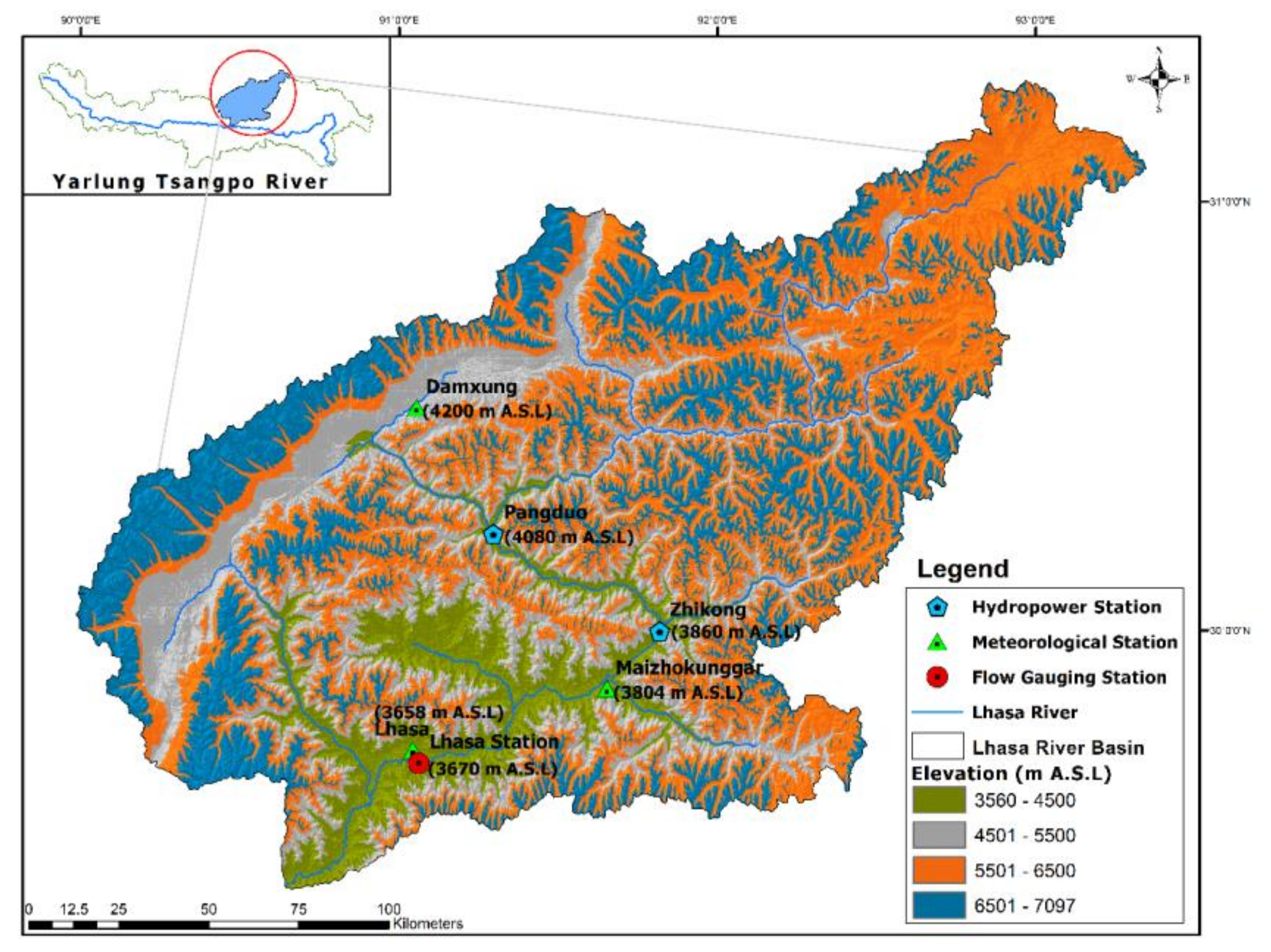
Figure 1. Digital Elevation Model (DEM) of Lhasa River Basin showing river network, hydropower station, meteorological stations and flow gauging stations.
Water 12 01370 g001
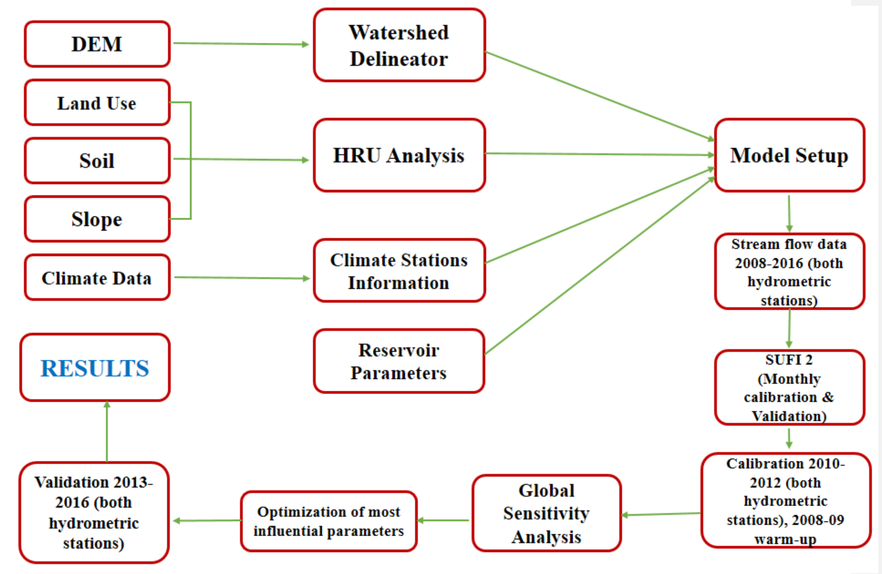
Figure 2. Schematic representation of Soil and Water Assessment Tool (SWAT) model setup for the current study.
Water 12 01370 g002
Figure 3. (a) Soil and (b) land use data raster for Lhasa River Basin.
Water 12 01370 g003
Figure 4. Flow-duration curves for the annual Lhasa River discharge for 2008–2016 observed at Pondo and Lhasa flow gauging stations. The reservoir impoundment year is marked.
Water 12 01370 g004
Figure 5. Monthly Lhasa River observed discharge at Pondo and Lhasa flow gauging stations, 2008–2016.
Water 12 01370 g005
Figure 6. Mann–Kendall trend test on (a) seasonal rainfall and streamflow recorded at Pondo flow gauge and (b) seasonal rainfall and streamflow recorded at Lhasa flow gauge.
Water 12 01370 g006
Figure 7. Hydrograph of monthly discharge calibration (2010–2012) and validation of Lhasa River (2013–2016), showing the simulated and observed monthly streamflow at Pondo flow gauging station.
Water 12 01370 g007
Figure 8. Hydrograph of monthly discharge calibration (2010–2012) and validation of Lhasa River (2013–2016), showing the simulated and observed monthly streamflow at Lhasa flow gauging station.
Water 12 01370 g008
Figure 9. Percent change in monthly observed and simulated streamflow at Pondo flow gauge as a consequence of Pangduo reservoir functioning.
Water 12 01370 g009
Figure 10. Percent change in monthly observed and simulated streamflow at Lhasa flow gauge as a consequence of Pangduo reservoir functioning.
Water 12 01370 g010
Figure 11. Reservoir water level and observed and simulated Lhasa River discharge at Pondo (left) and Lhasa (right) flow gauge stations for the year 2015.
Water 12 01370 g011
Figure 12. Pangduo Reservoir inflow and observed and simulated river discharge at Pondo flow gauging station for the years 2015–2016.
Water 12 01370 g012
Table 1. Pangduo reservoir specifications.
Reservoir SpecificationDetail
total storage capacity of the reservoir (volume of water when the emergency spillway is filled)1.23 billion cubic meters
adjusted storage capacity (volume of water when the principal spillway is filled)811 million cubic meters
dead storage capacity271 million cubic meters
normal water level4095 m
dead water level4066 m
restricted water level during the flood4093.5 m
maximum dam height72.30 m
elevation of the dam at top4100.00 m
dam length1052 m
total installed capacity160 MW
Table 2. Sensitive Parameters for stream flow simulation in Lhasa River Basin at the selected hydrometric stations.
No.ParameterParameter DescriptionMethod Chosen
1.CN2Initial SCS curve number for soil condition IIRelative
2.GW_DELAYGround water delay (days)Replace
3.GW_REVAPGround water “revap” coefficientReplace
4.ESCOSoil evaporation compensation factorReplace
5.EPCOPlant uptake compensation factorReplace
6.SOL_BDSoil bulk density (mg/m3)Relative
7.SOL_KSaturated hydraulic conductivity (mm/h)Relative
8.SOL_AWCAvailable water capacity of soil layer (mm H2O/mm soil)Relative
9.OV_NManning’s “n” value for overland flowRelative
Table 3. Calibration flow parameter range with lower and upper boundaries, fitted value, rank, t-stat and p-value for monthly river discharge simulation of Lhasa River at Pondo flow gauging station.
ParameterRangeFitted ValueRankt-statp-Value
MinMax
r__SOL_K−0.80.5−0.3012.6010.017
r__SOL_BD01.50.6221.6060.123
v__GW_DELAY1505001673−1.4880.152
r__CN2−0.5−0.1−0.244−1.3920.179
r__SOL_AWC−0.90.1−0.1151.2460.226
v__GW_REVAP0.50.90.7760.8980.379
v__ESCO−0.80.2−0.417−0.7530.459
v__EPCO−0.10.8−0.058−0.2870.776
r__OV_N−0.30.50.0390.1670.868
Table 4. Calibration flow parameter range with lower and upper boundaries, fitted value, rank, t-stat and p-value for monthly river discharge simulation of Lhasa River at Lhasa flow gauge station.
ParameterRangeFitted ValueRankt-statp-Value
MinMax
r__SOL_BD−110.84124.3980.000
r__SOL_K−11−0.39218.2430.000
r__CN2−0.25−0.01−0.20310.7610.000
v__ESCO0.0110.9043.4200.000
r__SOL_AWC−11−0.565−2.3000.021
v__GW_REVAP0.020.10.066−1.5820.114
v__GW_DELAY1505004787−1.5540.120
v__EPCO010.7980.3240.745
r__OV_N−11−0.049−0.2770.781