1. Introduction
Digital elevation models (DEMs) have been widely used in many fields such as landform evolution, soil erosion modeling, and other geo-simulations [
1,
2,
3,
4]. In particular, DEMs provide indispensable data to support water resource management and flood risk assessment [
5,
6]. In urban flood risk assessment, the availability of high-resolution urban DEMs is crucial for the accurate representation of complex urban topographic features and is required for a reliable prediction of flood inundation to inform risk calculation [
7,
8].
The common ways of acquiring high-resolution urban DEMs include ground surveying and remote sensing through light detection and ranging (LiDAR) [
9,
10]. For LiDAR data in particular, many data filtering and fusion methods for improving data quality have been developed to support urban flood modelling to achieve better performance [
11,
12,
13,
14,
15]. However, these LiDAR data processing methods are usually applied on high-resolution topographic datasets, and cannot create high-resolution DEMs from low-resolution data. Meanwhile, these data acquisition approaches are usually labor-intensive and financially expensive, hindering their wider application across a large domain. As such, high-resolution urban DEMs are not always available, especially for cities in developing countries. This essentially imposes a barrier for many applications including the development of effective urban flood risk management strategies that are necessary to be informed by high-resolution flood modelling results. Hence, it is necessary to develop alternative and more cost-effective approaches to construct high-resolution urban DEMs to support a wide range of applications.
Although high-resolution urban DEMs are not always available, low-resolution DEMs, on the other hand, are relatively easy to access. For example, there are a range of open-access global or regional DEMs, including Shuttle Radar Topography Mission (SRTM), ALOS World 3D, and pan-Arctic DEM [
16]. Many relevant studies, such as CoastalDEM, show that these datasets provide important resources for water engineering applications including region-scale flood modelling and risk analysis [
17,
18]. However, the resolution of these open datasets is not sufficient to depict urban topographic features, including buildings and street networks, to support high-resolution flood modelling. Thus, it is desirable to develop effective techniques to enhance the quality of low-resolution DEMs to subsequently obtain high-resolution urban DEMs. Most of the existing high-resolution DEM reconstruction methods are developed for natural terrains, which may be generally classified into three categories: DEM interpolation, DEM enhancement, and learning-based DEM reconstruction.
The DEM interpolation methods, commonly including inverse distance weighting (IDW), bilinear interpolation (BI), cubic convolution (CC), and kriging interpolation (KI), are generally implemented according to spatial autocorrelation, that is, the correlation of the ground elevations between two points is inverse to the distance between them (also known as Tobler’s first law of geography) [
19,
20,
21,
22,
23]. These methods have been widely applied to generate high-resolution DEMs, but they commonly smoothen the fine topographic details (i.e., high frequency details) and lead to blurry information in the output products. To relax the limitation of these DEM interpolation methods, DEM enhancement methods are developed to restore the lost topographic features via introducing extra information to enhance the quality of low-resolution DEMs. The extra information may be derived from additional elevation points, contours, land-use maps, and flood extents [
24,
25,
26,
27,
28], among others. DEM enhancement methods may improve the resolution and accuracy of DEMs by fusing multiple DEMs and datasets of different resolutions and from various sources. Nevertheless, the required extra-high-accuracy topographic information for the implementation of this type of method is still hard to acquire, especially for a large extent. The learning-based approaches generate high-resolution DEMs by establishing the correlation between low- and high-resolution DEMs through a training process [
29,
30,
31,
32,
33]. Learning-based models can be trained to learn from multi-dimensional information, which may potentially produce high-resolution DEMs of better quality. However, less research has been done in this direction, and the existing learning-based models are relatively simple and not suitable for application in complex urban environments.
Most of the existing DEM reconstruction methods are developed and applied in natural terrains. Reconstruction of urban high-resolution DEMs faces extra challenges, and direct application of the existing methods in the complex urban environments is questionable and may not be feasible. Due to human interventions, urban topography is typically an intricate synthesis of natural and artificial features (e.g., roads, buildings, and different types of vegetation covers). For flood modelling, these key urban structures/features commonly define flood pathways and predominantly control the underlying hydrological and inundation processes, and must be accurately represented in urban DEMs to produce reliable simulation results [
34,
35,
36]. Basically, the resolution of the topographic data must be consistent with the scale of the involved processes to ensure they can be reliably modelled and correctly interpreted [
37]. Therefore, there is a strong research and practical need to develop new approaches to support multi-scale DEM reconstruction and efficiently reconstruct urban DEMs at a specified higher resolution from a low-resolution equivalent to support more accurate urban flood modeling and other applications.
Although cities are widely covered by artificial topographic features of different types and scales, they are planned and built according to specific regulations and codes. In other words, urban topography commonly presents a high level of self-similar structures or features, especially for cities in the same region. This is particularly suitable for the application of learning-based approaches. For example, convolutional neural network (CNN) [
38,
39] is a deep learning technique designed to automatically and adaptively learn the spatial hierarchies of image features and has been successfully applied in image recognition and many other fields, such as machine translation and autonomous driving [
40,
41,
42]. An urban gridded DEM can be effectively regarded as an image. Using localized urban DEMs of different resolutions, a CNN model may be trained to recognize the patterns of topographic features varying from high to low resolutions or vice versa, and subsequently used to reconstruct high-resolution DEMs from the low-resolution data across a large area. Although it is challenging and expensive to create high-resolution DEMs across a large area covering an entire city, it is more feasible to acquire high-resolution DEMs in localized (small) areas using a range of survey techniques, such as an unmanned aerial vehicle (UAV). This paper presents an innovative multi-scale approach using a deep-learning CNN model to reconstruct high-resolution urban DEMs from a low-resolution dataset. To our best knowledge, this is the first attempt to construct a CNN-based multi-scale mapping framework for efficiently enhancing the resolution of urban DEMs, which may contribute to resolving the issue of data-scarcity for urban flood modelling and water engineering applications.
The rest of this paper is arranged as follows:
Section 2 introduces the proposed multi-scale mapping approach for urban DEM reconstruction, followed by the introduction of a two-level accuracy assessment framework in
Section 3;
Section 4 describes the experiments undertaken to validate the proposed high-resolution urban DEM reconstruction approach; further discussion is given in
Section 5; and finally several remarks are summarized in
Section 6.
2. A CNN-Based Multi-Scale Mapping Approach
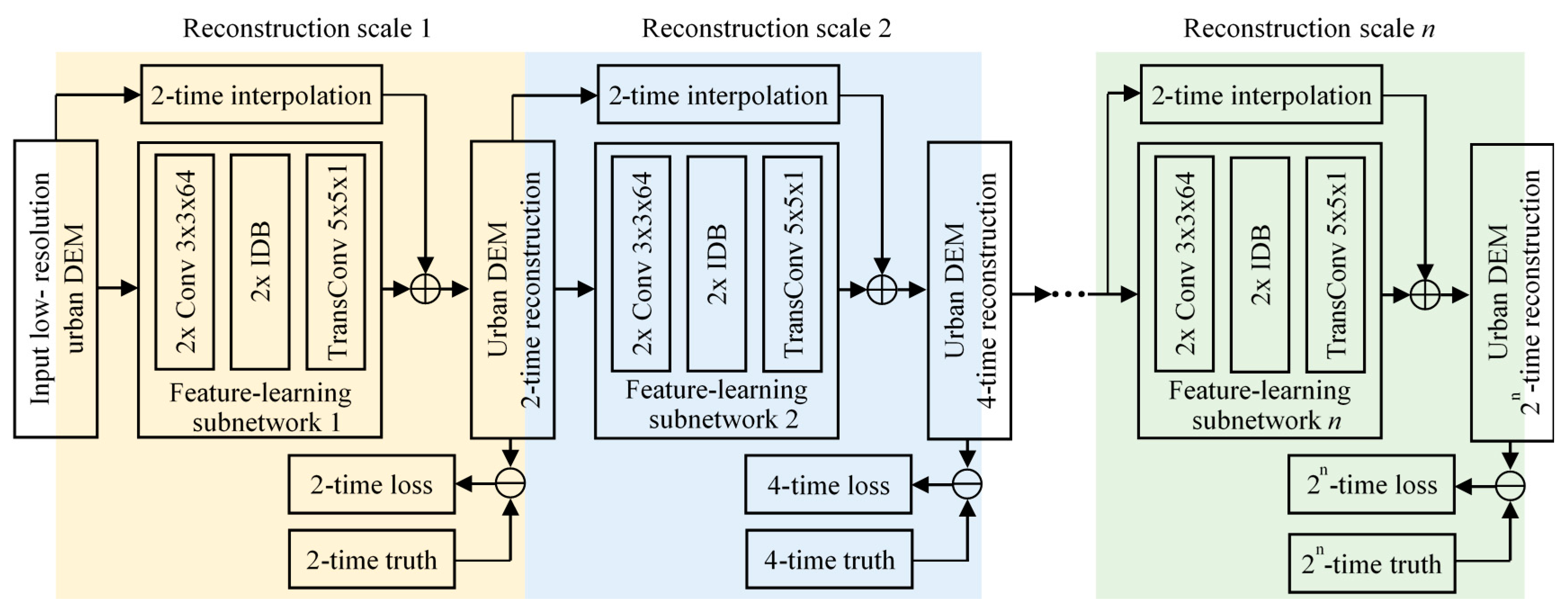
A multi-scale mapping approach based on CNN (MSM-CNN) was developed in this work to reconstruct high-resolution urban DEMs from a low-resolution dataset, which is illustrated in
Figure 1 and
Figure 2. Herein, the low-resolution DEM is denoted as
X, and the corresponding datasets at higher resolutions are denoted as
,
,…,
, where the superscript 2
n indicates that these DEMs are at 2
n times higher resolution than the low-resolution DEM
X, and
n is a positive integer. The goal here was to reconstruct an urban DEM
at a higher resolution from the low-resolution DEM
X to ensure that
was as close to the ground truth dataset
as possible, which was achieved by training a CNN to learn mapping
F.
2.1. Network Architecture
The detailed network architecture is shown in
Figure 1, which consists of several subnetworks. Each of these subnetworks performs a 2-time reconstruction to its input urban DEM. According to the existing state-of-the-art results, a network with skip connections bypassing certain intermediate layers may lead to better performance [
43,
44,
45]. Therefore, we introduced skip connections between the input and output of each of the subnetworks. Specifically, the input urban DEM of each subnetwork is interpolated to become two times its original resolution using a nearest neighbor (NN) method, and the interpolated data are then directly summed to the output of the feature-learning network. NN here was chosen due to its computational efficiency compared to other interpolation methods. The skip connections encourage the feature-learning networks to effectively learn and predict the missing topographic details from the low-resolution datasets to generate high-resolution datasets. Because each subnetwork only performs a 2-time reconstruction, the proposed architecture can effectively train a single network to construct urban DEMs at different higher resolutions.
In the proposed architecture, the feature-learning network is a key component in each of the subnetworks. Each feature-learning network starts with two convolutional layers with the kernel size specified as in
Figure 1. The effect of the two convolutional layers is to extract initial features for further feature learning. The first two convolutional layers in the feature-learning network are followed by two information distillation blocks (IDBs) [
46] to learn more powerful deep features for urban DEM reconstruction. The architecture of IDB is presented in
Figure 2. The IDB starts with a stack of six convolutional layers, with the filter size specified as in
Figure 2. After the first three layers in each IDB, the output feature maps are split into two parts. The 1−1/
s percent of the feature channels are used as the input to the next three layers, whereas the other 1/
s percent feature channels is directly concatenated with the output of the next three layers. Such a structure creates skip connections and combines features in both shallower and deeper layers. The output of the first six blocks in IDB is passed to a seventh convolutional layer. This convolutional layer with 1 × 1 filters acts similarly to a bottleneck layer [
47]; its effect is to combine and compress the shallow and deep features’ output by the previous layers. Herein, although we used IDB as the backbone of the proposed network, other architectures could potentially also be used to replace IDB for feature learning. This paper focused on developing an innovative multi-scale network for urban DEM reconstruction rather than seeking the backbone architecture with the best performance; we selected IDB due to its reported excellent performance in accuracy and efficiency in computational cost. After the two IDBs, a transposed convolutional layer was applied to project the output feature maps of a subnetwork to a reconstruction at 2-time resolution with respect to the input of this subnetwork.
The proposed network uses rectified linear unit (ReLU) activation function, formulated as
y =
max (0,
x), where
x represents the input feature maps and
y the output;
y is equal to
x if
x is positive, otherwise
y is 0. ReLU was adopted due to its widely reported effectiveness in the literature [
43,
44,
45]. Herein, all of the convolutional layers are followed by a ReLU unless it is specifically mentioned otherwise.
A key advantage of the proposed multiple-scale architecture with respect to a single-scale architecture is that the multi-scale supervision was introduced to regularize the intermediate features of an urban DEM, which can faithfully enhance the output of each subnetwork to become as close to the high-resolution “true” DEM as possible. The adopted multi-scale supervision enables effortless and effective reconstruction of urban DEMs with enhanced accuracy at any specified higher resolution. Note that multi-scale design and computing losses at the intermediate network layers to guide the learning process have been widely used in deep neural network architectures [
47,
48,
49,
50]. In this paper, for the first time, we introduced this principle to the topic of urban DEM reconstruction.
2.2. Loss Function
The loss function used to train the network is based on mean absolute error (MAE). Let
Yi be the 2
i-time reconstruction result and
Ri be the corresponding ground truth. The overall loss of network training denoted by MAE
loss is calculated as follows:
where
Ri,j and
Yi,j are the element in
Ri and
Yi, respectively;
C is the cell number; and
n is the number of higher resolution datasets in the multi-scale gradual network.
Theoretically, a weighted sum could achieve better balance among the losses at different reconstructed resolutions. However, preliminary experiments reveal that the sum loss with equal weights is sufficient to achieve a good performance. We also compared the other metrics (e.g., mean squared error, structure similarity index, and peak signal-to-noise ratio) with MAE. MAE is not sensitive towards outliers and encourages less blurry surfaces, which is beneficial to reconstruct the spatial relationship between different artificial objects (e.g., roads and buildings) in urban terrains from the low-resolution data.
2.3. Network Training and Validation
We trained all the layers in the proposed network from scratch on the basis of the standard backpropagation with Adam optimizer [
51] over a Caffe deep learning framework. The weights for convolutional layers were initialized using the method reported in [
52]. The weight decay was set to 0.0001, and the learning rate was set to 0.0001 initially and reduced by a factor of 10 after 250 thousand iterations.
Prior to training the model, we prepared the training data by sampling it from the three selected training areas (see
Section 4.1). Each of these sampled scenes had a spatial dimension of 500 by 500 cells and overlapped with neighboring scenes in both horizontal and vertical directions by 250 cells. The total number of sampled scenes available to train the model was 4107. A batch of 64 scenes was randomly selected from the sampled scenes that were from same training area, and then a patch from each scene was randomly cropped. These patches were then concatenated to form the batch of training data (i.e., we trained the model with a batch size of 64) during each forward–backward pass of the network. The size of a patch was chosen to meet the computational capacity, which depended on the number of scales in the network.
Upon successful completion of the training process, the first step was to examine whether the proposed method worked satisfactorily for scenes that had morphological characteristics similar to the training datasets. Therefore, a set of 456 scenes (not used during the training process) from the same three training areas was used to validate the model. However, investigating the generalization ability and transferability of the trained model in reconstructing high-resolution urban DEMs using spatially separated low-resolution data was more challenging. The effectiveness of the presented method over the test area is further analyzed in
Section 4.
3. Two-Level Accuracy Assessment
To evaluate the performance of the proposed urban DEM reconstruction method, a two-level assessment approach was designed to quantify the numerical accuracy and morphological accuracy of the resulting products. Herein, the numerical accuracy is a quantification of elevation error at the cell locations, whereas the morphological accuracy is a region-scale quantification of morphology variance between the reconstructed urban DEM and ground truth.
3.1. Numerical Accuracy
Numerical accuracy was assessed by quantifying the difference of pointwise elevation between the reconstructed and “true” urban DEMs. Three metrics—MAE, root mean square error (RMSE), and standard deviation (STD)—were employed to quantify the numerical accuracy, which have been used as the standard statistical metrics for DEM vertical accuracy assessment [
17,
53]. The related equations to define RMSE and STD are given as follows:
where
c is the total count of valid grid cells,
x denotes the ground elevations given by the reconstructed urban DEM, and
y refers to the reference values.
3.2. Morphological Accuracy
A DEM not only represents the ground elevation at each of its cells, but also reveals the structure of the topography. As the skeleton of topography, topographic structure decides the spatial pattern of geomorphology [
54]. Hence, the accuracy in representing the topographic structure is an essential indicator for DEM quality assessment. In the case of urban topography for application in flood or hydrological modelling, the topographic structure may be mainly reflected by the road networks and building clusters that have a significant impact on surface runoff and flow processes. Accordingly, the morphological accuracy, that is, the assessment of topographic feature difference, can be quantified by measuring the variances of the road profiles and building boundaries derived from the reconstructed urban DEM and the reference data.
The road-profile variance is measured through the following steps: (1) add vertices along each road centerline stepped by the cell size of the reconstructed urban DEM; (2) generate the road profiles respectively from the reconstructed and reference data; and (3) apply the Pearson’s correlation coefficient (PCC) to quantify the variance between two profiles for each of the roads in the study area, and use the average and STD of PCCs to define the difference. Herein, the first two steps are implemented on the ArcGIS platform, and the last step is done using the Excel. The PCC is calculated as follows:
where
m represents the number of the profile vertices, and
x and
y are the values corresponding to the reconstructed and reference profiles being compared.
On the ArcGIS platform, the variance of the building boundaries can be measured through three steps:
Step 1 is to consider the reference data by (1) preprocessing building polygons via merging the adjacent polygons and deleting those small and discrete patches according to an area threshold of 20 m2, (2) obtaining the reference boundary line of each building patch and converting all lines to a raster aligned with the reference data, and (3) counting the boundary cells as the reference truth.
Step 2 is to extract building boundaries from the reconstructed urban DEM by (1) enhancing edge features (e.g., the boundary where a building meets a road) by a high-pass filter, (2) screening the candidates of boundary cells via an edge threshold of 1, and (3) obtaining the boundary cells using a thinning tool.
Step 3 is to quantify the variance by (1) selecting the boundary cells from step 2 according to the location of the reference boundary lines with no buffer, and buffers of 1, 2, and 3 times of the cell size of the reference data, respectively, and (2) calculating the ratio between the number of selected cells and that of the reference truth from step 1 successively. Finally, these four ratios are used to quantify the building-boundary variance.
4. Experiments and Results
In order to validate the performance of the proposed MSM-CNN method, a series of simulation experiments were undertaken. In the experiments, the MSM-CNN model was trained and applied to reconstruct high-resolution urban DEMs in the case study area. The experiments were performed on a single GPU (i.e., graphics processing unit) server with Nvidia K80 GPUs.
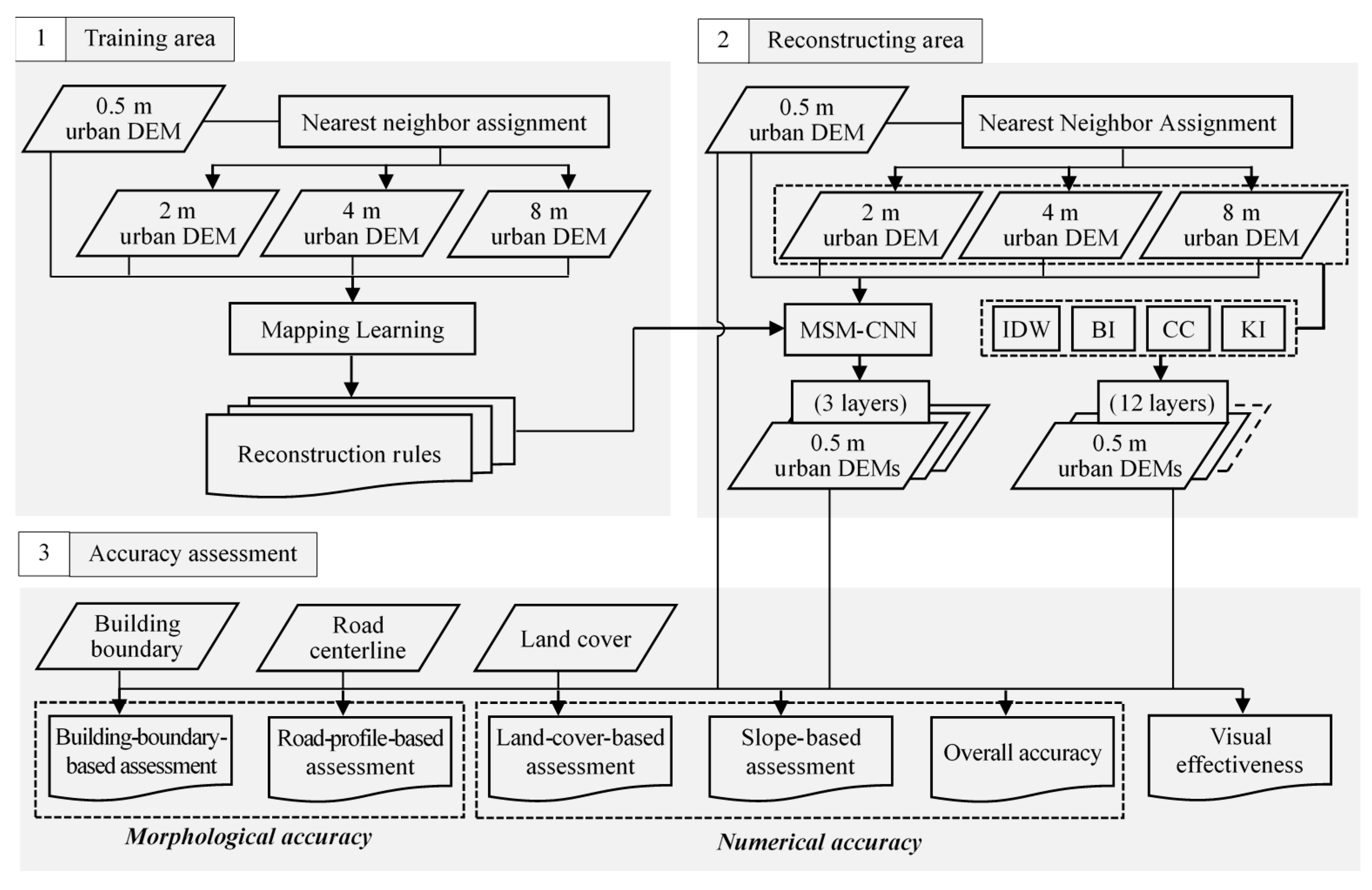
The produced outputs were compared with the results from several other popular interpolation or resample methods, including IDW, BI, CC, and KI. Herein, the ordinary KI was chosen due to its better accuracy among other types of KI for the study area. The experimental setup is illustrated in the flowchart shown in
Figure 3. In the experiments, the urban DEMs at low resolutions of 2, 4, and 8 m were used to reconstruct high-resolution urban DEMs of 0.5 m to evaluate the performance of the multi-scale gradual network. It should be pointed out that, due to the lack of real datasets of 2, 4, and 8 m in the same period, we generated the three datasets by resampling 0.5 m data to ensure the consistency of evaluation benchmark. Herein, in the reconstructing phase, the test dataset was divided into scenes with a size of 250 by 250 cells (including an overlap of 125 cells with their neighbors), and finally, each scene was constructed individually and combined together to obtain the reconstructed urban DEM.
4.1. Study Area and Data
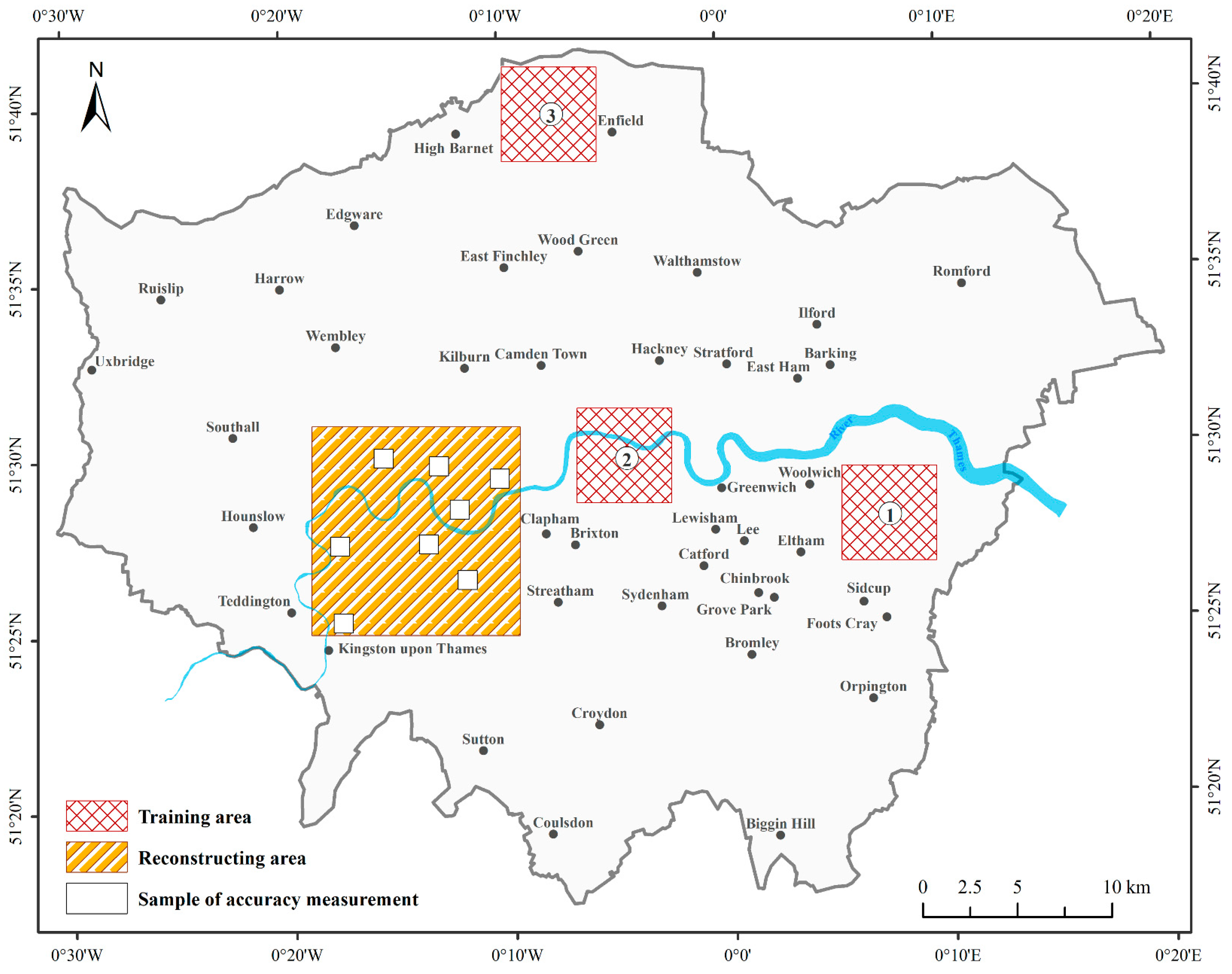
As one of the largest cities in the world, London, United Kingdom, is highly urbanized, with a population of 8 million, and was selected as the study area in this work. We firstly trained the MSM-CNN model using three small areas in the city. The three chosen training areas with significant different topographical features are located in the suburban, urban and rural regions, respectively. Each training site covered a 5 by 5 km area. After being trained, the MSM-CNN model was applied to reconstruct high-resolution DEMs in another larger area of 121 km
2, which is an urbanized area with mixed topographic features. The rationale to perform training and testing in different areas was that, although the overall urban designs could vary in different areas, the local features such as lines, edges, and blocks are similar across different natural and manmade structures; because a CNN focuses on local features, it could be used to reconstruct the urban structures in an area that is unseen in the training data. In this reconstructed area, eight samples of 1 by 1 km blocks were selected to facilitate morphological accuracy assessment.
Figure 4 shows the locations of the training, reconstruction, and sample areas in the City of London.
In this work, a 0.5 m LiDAR DSM was used as the baseline high-resolution urban DEM, which is published by the Environment Agency, United Kingdom (
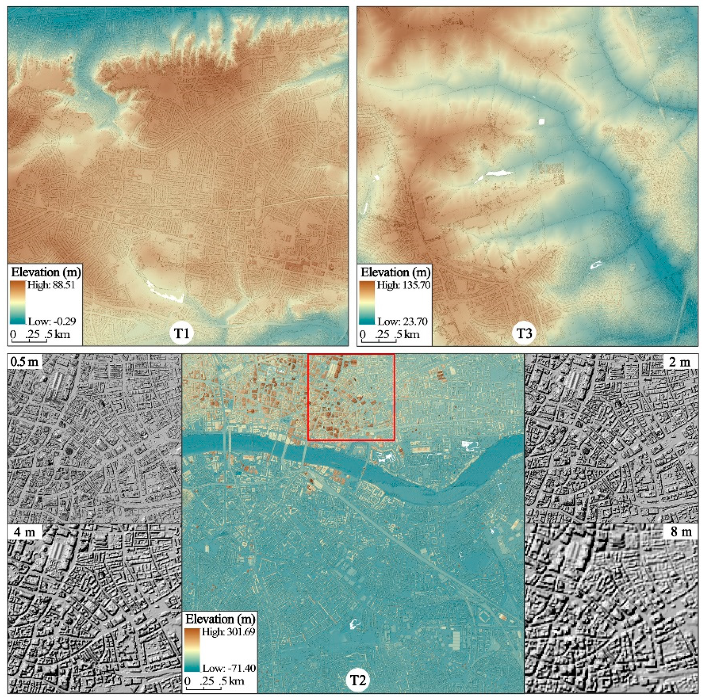
https://environment.data.gov.uk/ds/ survey/index.jsp#/survey). This dataset was employed for training the MSM-CNN model, and was used as the reference truth for assessing the reconstruction accuracy. The low-resolution DEMs for training and testing the MSM-CNN model were obtained from this 0.5 m DEM by resampling it to 2, 4, and 8 m resolutions using NN down-sampling (
Figure 5). We selected NN instead of other alternative approaches such as BI or CC because this paper focused on urban DEM, which includes a large amount of abrupt elevation changes (e.g., a road with high buildings at both sides). For these specific types of data, methods such as BI and CC could be less suitable compared to NN, as they introduce “fake” elevation for the areas with abrupt features. Other relevant datasets of land cover, road centerline, and building were downloaded from Digimap (
https://digimap.edina.ac.uk) for use in the current study. All of the above geospatial data were in the same coordinate reference system. It should be noted that if the coordinate reference systems of the essential data for MSM-CNN are different, geo-referencing (also known as image alignment) must be performed first.
4.2. Visual Assessment
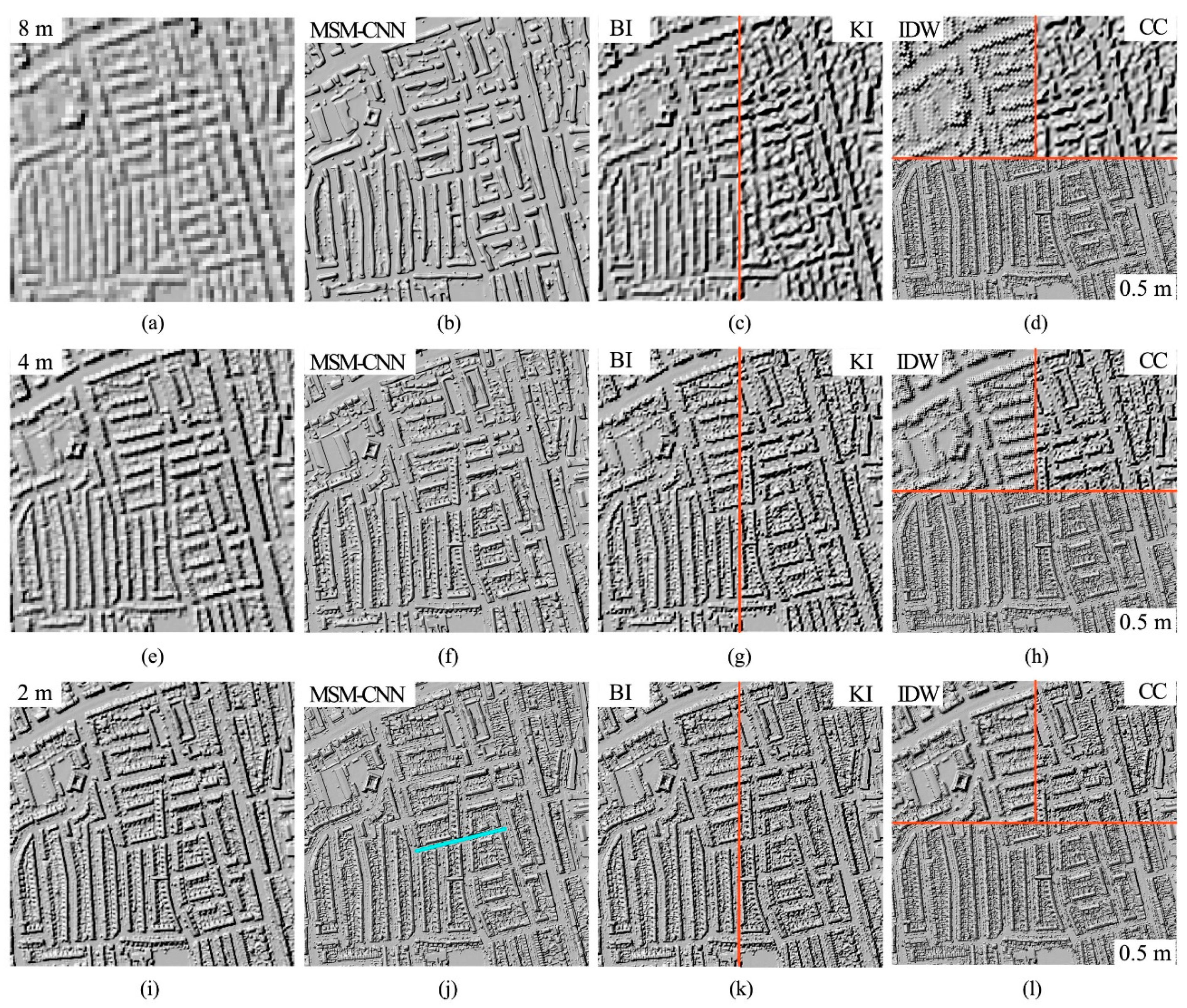
The 0.5 m urban DEMs reconstructed using different methods were plotted together with the low-resolution counterparts of 8, 4, and 2 m in
Figure 6. Naturally, the detailed features of urban topography were gradually lost as the resolution of the DEMs reduced from 0.5 to 2, 4, and 8 m (
Figure 6a,e,i). The topographic structures related to road networks and building groups became blurry when the DEM resolution decreased. On the 8 m DEM, the roads and buildings became hard to identify. As depicted in
Figure 6c,d,g,h,k,l, the BI, KI, CC, and IDW interpolation methods provided a certain level of enhancement in the topographic details. However, the level of enhancement was generally very limited, and in particular, it was not possible to restore most of the topographic structures from the lowest resolution (8 m) urban DEM. Moreover, hillock-like features were created in the three sets of the IDW reconstruction results, which did not conform to the morphological cognition of urban topography. It may be concluded that IDW is not applicable to urban topography, and IDW was therefore not chosen to support further accuracy assessment.
The MSM-CNN evidently achieved better results for the reconstructions from all of the three low-resolution urban DEMs (
Figure 6b,f,j). In the whole area, the topographic structure was restored remarkably well, especially for the result reconstructed from the low-resolution DEM of 8 m, which showed good fidelity to the actual terrain. The MSM-CNN reconstructed DEM well represented both the continuous and abrupt features. Locally, the buildings and roads were clearly reconstructed, with their boundaries consistent with the reference terrain. As expected, the restored level of topographic details greatly depended on the input low-resolution urban DEMs, and more details were shown in the DEMs reconstructed from input datasets of higher resolutions. The results indicated that MSM-CNN can effectively achieve the multi-scale reconstruction to enhance the quality of low-resolution urban DEMs.
4.3. Numerical Accuracy
4.3.1. Overall Accuracy Analysis
Taking the original 0.5 m urban DEM as a reference, the results of numerical accuracy assessment of different reconstruction methods are listed in
Table 1. From the 2 m low-resolution urban DEM, the 0.5 m product reconstructed by MSM-CNN was the most accurate, confirmed by the lowest MAE (0.194 m) and RMSE (0.918 m); meanwhile, the least accurate reconstruction result was obtained by CC, which had the highest MAE (0.234 m) and RMSE (1.028 m). The products reconstructed by BI and KI had the same MAE (0.234 m) but slightly different RMSEs of 1.012 and 1.019 m, respectively. From the lower-resolution DEM of 4 m, the best reconstruction result was still obtained by MSM-CNN, having MAE of 0.316 m and RMSE of 1.295 m. For the results reconstructed from the lowest-resolution dataset of 8 m, the MAE of the MSM-CNN reconstruction was slightly inferior to that of BI, but better than that of CC and KI; MSM-CNN also returned similar, but with slightly higher RMSE than BI and CC, and slightly lower value than KI.
Overall, the numerical accuracy of the MSM-CNN reconstructions was mostly higher than that achieved by other interpolation methods. Meanwhile, it was noted that the variances of the numerical accuracy between MSM-CNN and other interpolation methods were not significant, which appeared to contrast with the visual comparison of the reconstruction results presented in
Figure 5. The reason may be that the local elevation variation of urban topography in the reconstructing area was relatively small, and the overall statistics may not have efficiently reflected the small differences. It was therefore necessary to further investigate the performance of the MSM-CNN model by considering the morphological accuracy as well as conducting numerical accuracy assessment in groups, such as slope ranges and land covers.
4.3.2. Vertical Accuracy based on Slope Classification
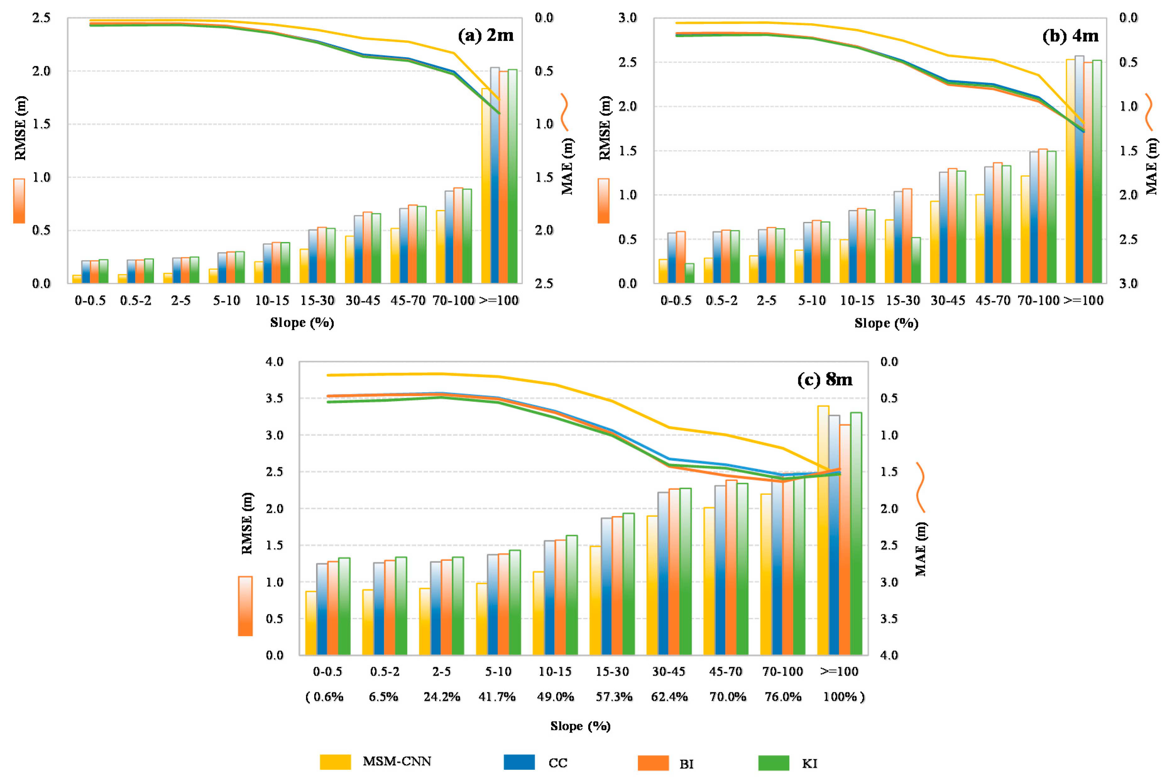
We further investigated the vertical accuracy of the reconstruction methods by considering slope classification. The topographic features were divided into 10 ranges according to the ground surface slopes, and then MAE and RMSE were respectively calculated for each of these ranges (
Figure 7).
Table 2 lists the average MAEs and RMSEs for all of the 10 slope ranges. Herein, the slope data were derived from the original 0.5 m urban DEM. From
Figure 7a–c, a general increasing trend can be observed for both MAEs and RMSEs calculated for the different reconstruction results as the slope gradually increased. This indicated that the urban terrain relief as indicated by the slope factor had an obvious influence on the vertical accuracy of DEM reconstruction. As shown in
Table 2, among all four approaches, MSM-CNN returned the highest accuracy confirmed by low RMSE and MAE for the reconstructions from all of the adopted low-resolution DEMs. The superior accuracy was maintained across all slope ranges until the slope was ≥ 100%, which covered 76% of the whole reconstruction area.
As the slope of the topography increased to ≥ 100%, both MAE and RMSE of the MSM-CNN reconstruction results were slightly higher than those of the other three methods when the reconstruction was conducted for the low-resolution DEM of 8 m. The MAEs of the BI, CC, and KI reconstruction results from the 8 m dataset started to decrease as the slope went beyond 100%, whereas the their RMSEs continued to increase. In cities, the areas with the slope ≥ 100% are mostly featured with abrupt change of terrain. Therefore, the reasons for the two aforementioned abnormalities may have been because the 8 m low-resolution urban DEM had smoothened out those sharp-fronted topographic features in this area, leading to the disappearance of the abrupt urban topography. As such, the MSM-CNN model may have exaggerated the reconstruction error by maximizing the restoration of the abrupt characteristic. For BI, CC, and KI, they essentially smoothened the abrupt terrain during the reconstruction without recreating abrupt change of the topography. Because the area featured with this highest slope range of ≥ 100% took up 24% of the total area, the influence on the reconstruction results was evident. The findings may also explain the overall accuracy assessment result in
Table 1, where the MSM-CNN reconstruction result from the 8 m DEM was slightly less accurate than those obtained using other interpolation methods.
4.3.3. Vertical Accuracy based on Land Cover Classification
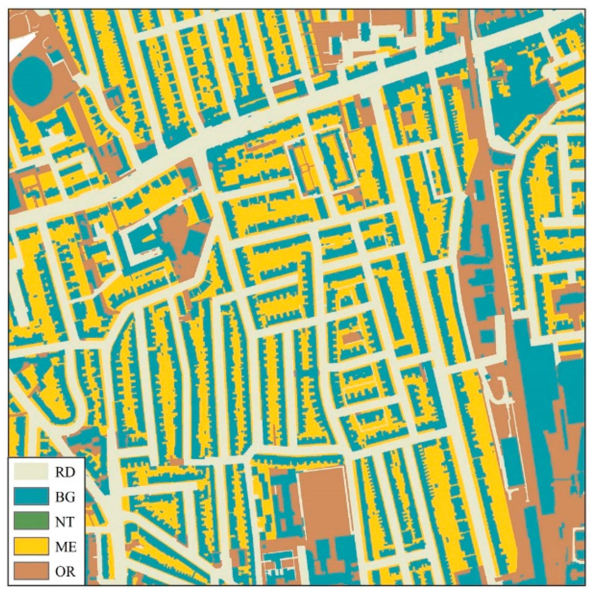
For urban topography, terrain change is closely related to land cover types. Therefore, the vertical accuracy of the reconstructed DEMs from different approaches was also analyzed for various types of land covers. Herein, the urban land covers were divided into five types for analysis, including roads (RD), buildings (BG), natural environments (NT), multi-surfaces (ME), and others (OR). NT included those areas representing geographic extents of natural environments and terrains. ME comprised all of the artificial surfaces that are mainly around buildings, such as yards and plazas. Except for the first four types, the rest were classified as OR.
Figure 8 illustrates the distribution of different land covers in a sample area within the case study site.
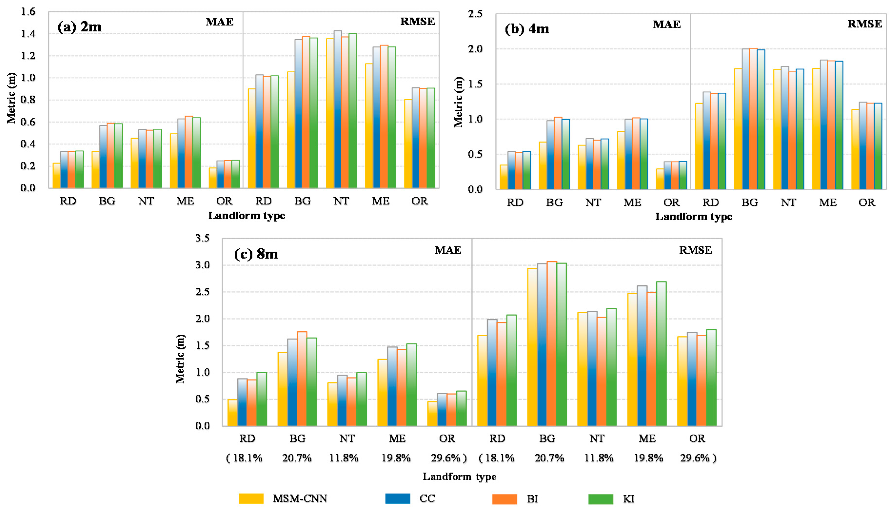
Figure 9 shows the statistics of MAE and RMSE across different land covers for each of the reconstructed DEMs. For all of the land cover types, MSM-CNN returns smaller MAEs than all other alternative approaches for all of the reconstruction experiments. However, for NT, the MSM-CNN products reconstructed from the 4 and 8 DEMs only gave slightly higher RMSE than the results produced by BI. This again demonstrated that MSM-CNN is well applicable to both natural and artificial terrain in urbanized cities, whereas the interpolation methods were more suitable for application to natural terrain, and did not produce favorable results for urban topography. It is interesting to note that for land cover types of RD and BG, the MAEs of the MSM-CNN DEMs reconstructed from all three low-resolution DEMs were much smaller than other reconstruction results. Obviously, these were the two major land cover types in the urbanized areas and covered approximately 40% of the total area in the current study site. The performance analysis results effectively demonstrated that the current MSM-CNN approach offered better capability in restoring urban topographic structures with a high fidelity. In addition, the errors calculated for ME were relatively high for all reconstruction results, although the corresponding topography inherently had a low relief. A possible reason may have been that vegetation was not removed from the original 0.5 m urban DEM created from LiDAR data. Vegetation cover may have significantly affected the reconstruction accuracy because its elevation changed disorderly and behaved like random noise, which is difficult to be reliably reconstructed from low-resolution DEMs.
4.4. Morphological Accuracy
4.4.1. Accuracy Assessment Based on Road Profiles
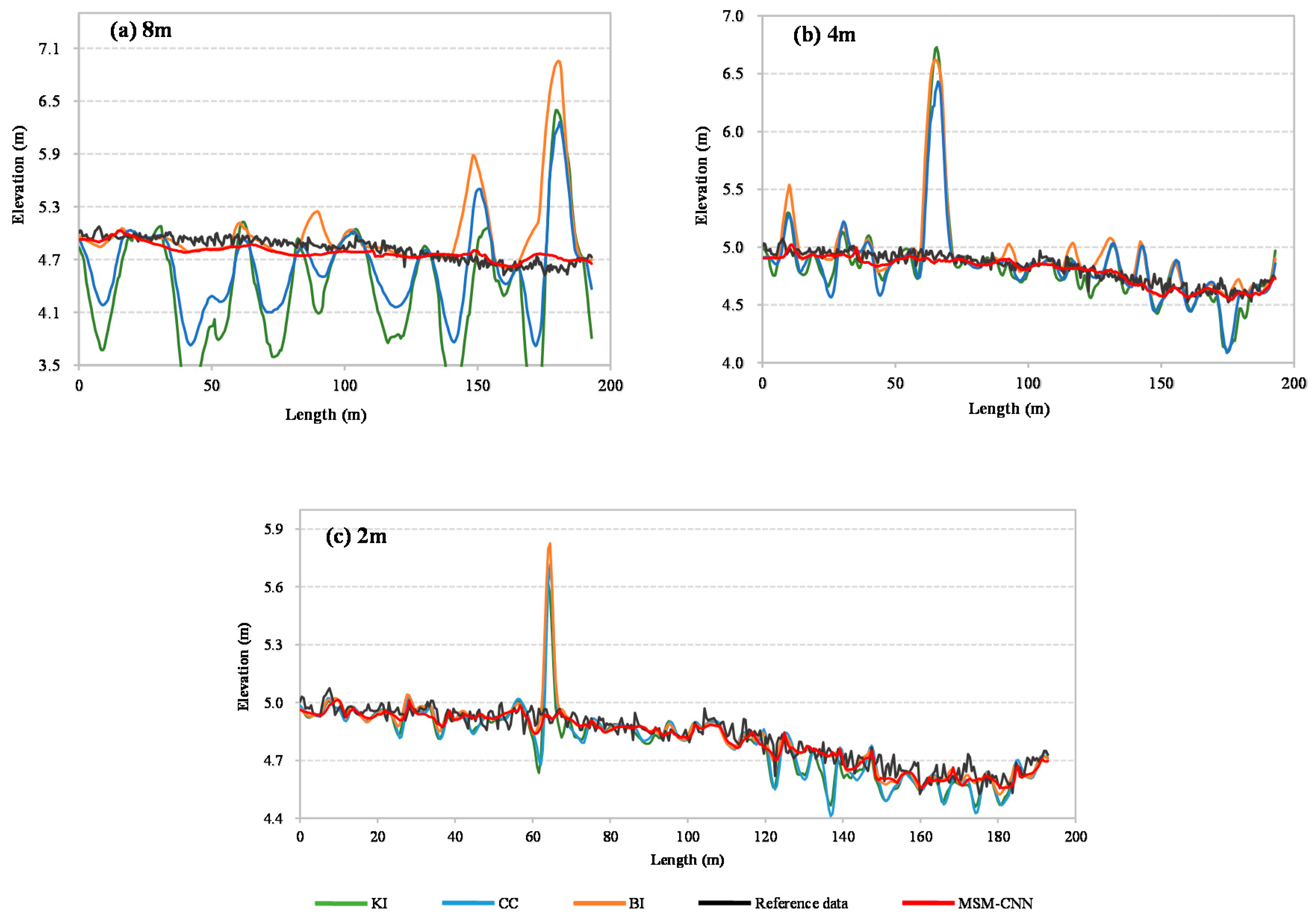
Figure 10 illustrates the centerline profiles of a road extracted from different reconstructed DEMs. The location of the selected road section is shown in
Figure 6j. Obviously, the detailed features of urban topography were gradually lost as the resolution of DEMs reduced from 0.5 to 2, 4, and 8 m (
Figure 6a,e,i), leading to blurry topographic structures related to road networks and buildings. Comparing the results obtained using different reconstruction methods, the MSM-CNN road profiles reconstructed from all three lower-resolution urban DEMs showed great agreement with the reference profiles extracted from the original 0.5 m dataset. On the contrary, the road profiles generated by BI, CC, and KI showed spurious oscillations that were inconsistent with the morphology of urban roads. In particular, for the reconstructed results from the lower-resolution 4 or 8 m urban DEMs, the oscillations in the BI, CC, and KI products were so strong that the centerline profiles were no longer recognizeable as a road. The potential reason for these results may have been that the BI, CC, and KI interpolation methods were implemented according to the spatial correlations between neighbors, whereas MSM-CNN was performed by the learned multi-dimensional patterns of topographic features varying from the high to low resolutions. When the DEM resolution decreased, the cell location where the prediction was being made had weaker or no clear spatial correlation with its neighbors. As such, the three CC or KI road profiles unexpectedly showed many deep ditches, which were again inconsistent with normal urban road morphology. The results confirmed the superior capability of the proposed MSM-CNN model in reliably reproducing urban morphology.
On the basis of the previous accuracy assessment results, BI produced better reconstruction results than the other two interpolation methods. Therefore, the following analysis was focused on comparing the morphological accuracy between the MSM-CNN and BI reconstruction results.
Table 3 summarizes the statistics of the road-profile variance to quantify the morphological accuracy of the results. For the 4-time reconstructions (i.e., the 0.5 urban DEMs reconstructed from the 2 m equivalent), MSM-CNN clearly gave a better result than BI. According to the PCCs calculated for the reconstructed road profiles, 51% of the MSM-CNN reconstructed profiles had a PCC greater than 0.95, whereas only 38% of the BI reconstructed profiles reached the same level. For the MSM-CNN and BI reconstructions from the 4 m urban DEM, the difference in the morphological accuracy was significantly increased, as indicated by the average PCC of 0.79 for the MSM-CNN profiles and 0.66 for the BI profiles. Although 51% of the MSM-CNN reconstructed road profiles had the PCC greater than 0.9, only 29% of the BI profiles were able to reach this level. For 16-time reconstruction, that is, reconstructing the urban DEMs from 8 m coarse resolution to 0.5 m fine resolution, the improved morphological accuracy achieved by MSM-CNN became even more prominent, and an improvement of 42% was achieved when compared with BI. The results demonstrated that the advantage of MSM-CNN in improving the morphological accuracy as represented by road-profile variance became more distinct as the resolution of the input urban DEM became coarser. In summary, the MSM-CNN reconstruction could substantially enhance the quality of low-resolution urban DEMs through improving morphological accuracy.
4.4.2. Accuracy Evaluation Based on Building Boundary Reconstruction
Using the extraction method described in
Section 3.2, building boundaries were delineated from the MSM-CNN and BI reconstructed DEMs for comparison, as shown in
Figure 11, in which the reference boundary data are also presented in the vector format. As shown in
Figure 11a for the 16-time reconstructions, the overall shapes of the boundaries were reasonably well reproduced by MSM-CNN, although certain fine-level details were smoothened out, which was as expected. However, almost no building boundary could be detected from the BI reconstructions.
Figure 11b illustrates the reconstructions from the 4 m DEM. MSM-CNN representation of building boundaries was further improved and building corners could be clearly recognized. However, BI still failed to reconstruct the overall shape of the building boundaries. As exhibited in
Figure 11c, the building boundaries in the MSM-CNN product reconstructed from the 2 m urban DEM were continuous and close to the reference, whereas the building boundaries produced by BI were typically segmented and did not align well with the reference. Evidently, MSM-CNN outperformed BI in restoring detailed features of urban topography and was more suitable for urban applications.
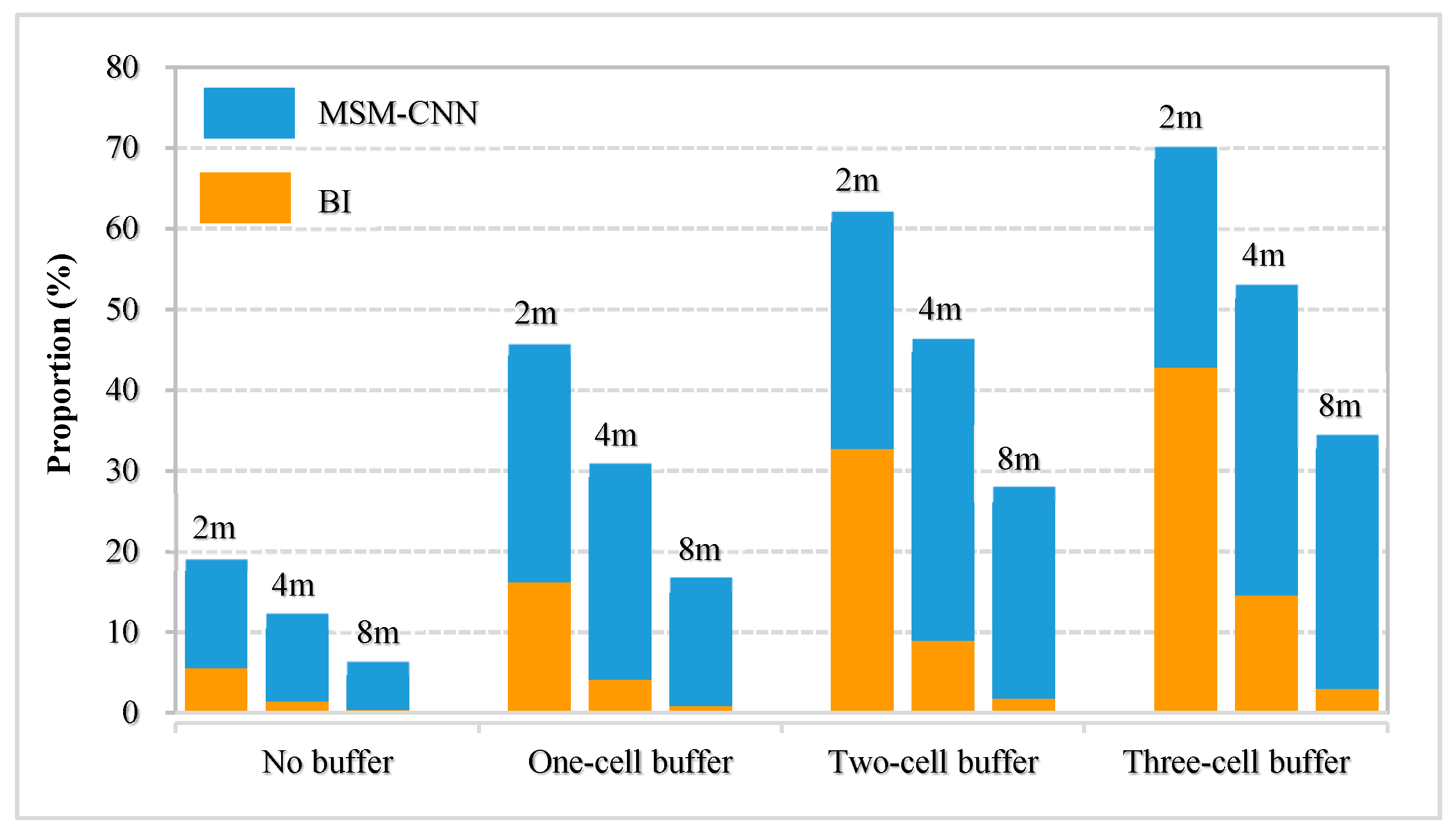
To quantify the morphological accuracy of building boundary reconstruction, the percentage of correctly restored boundary cells was calculated and plotted in
Figure 12. Overall, compared with BI, MSM-CNN presented clear superiority, especially for the reconstructions from lower-resolution DEMs. As expected, regardless the method being used, the morphological accuracy was calculated to be the highest for the 4-time reconstructions for each of the buffer ranges, followed by 8-time and 16-time reconstructions. The accuracy evaluated for the 4-time and 16-time MSM-CNN reconstructions only differed by an average of 2.5 times for the four buffer ranges. However, the accuracy difference unexpectedly reached 16.2 times for the corresponding BI reconstructions. When the buffer distance was chosen as three cells (approximately 2 m where the cell size was 0.5 m), the percentage of correctly restored boundary cells returned by MSM-CNN was 70.23% for the 4-time reconstruction, and 34.52% for 16-time reconstruction where the resolution of the input DEM (8 m) was nearly four times larger than the buffer distance. For BI, only 42.73% of the boundary cells were correctly restored by the 4-time reconstruction; for 16-time, the figure substantially dropped to only 2.91%. This effectively demonstrates that MSM-CNN consistently outperformed BI in restoring building details.
6. Conclusions
In this paper, we proposed an innovative deep machine learning approach to reconstruct high-resolution urban DEMs from low-resolution equivalents. In order to effectively account for the complexity of urban topography, a multi-scale CNN model was utilized to enhance the reconstruction quality. After the correlations between the low- and high-resolution urban DEMs are learned by the developed MSM-CNN model, an urban DEM at a specified high resolution can be accurately restored from a low-resolution dataset.
To evaluate the performance of MSM-CNN, a two-level accuracy assessment procedure involving both numerical accuracy and morphological accuracy was also designed and was used to compare the MSM-CNN with other DEM reconstruction methods including IDW, BI, CC, and KI. The results confirmed that MSM-CNN can effectively restore the high-resolution urban DEMs of 0.5 m from the low-resolution DEMs of 2, 4, and 8 m. The MSM-CNN products were also consistently better than those produced using alternative methods, in terms of visual assessment, and also numerical and morphological accuracy.
The promising results demonstrated that MSM-CNN provides a promising tool in generating high-resolution DEMs in cities from low-resolution DEMs, instead of surveying the whole region. In recent years, a number of global DEM products have been released to provide better resolution to represent urban topography, such as ALOS AW3D, NEXTMAP World 10, and WorldDEM. These open datasets can be explored and used to support the application of MSM-CNN to reconstruct high-resolution DEMs in cities across the world, which may potentially help address the challenging data scarcity issue and will have profound implications in many water-related applications, particularly in many of the developing countries.
