Article

A Generic Method for Predicting Environmental Concentrations of Hydraulic Fracturing Chemicals in Soil and Shallow Groundwater

1
CSIRO Land Water, Glen Osmond, SA 5064, Australia
2
CSIRO Land Water, Floreat, WA 6014, Australia
3
Departamento de Engenharia Sanitária e Ambiental, Federal University of Santa Catarina, Florianópolis 88040, Brazil
4
Schmidt Institute of Physics of the Earth of Russian Academy of Sciences, Moscow 123242, Russia
5
Department of Agriculture, Water and the Environment, Australian Government, Canberra 2600, Australia
*
Author to whom correspondence should be addressed.
Water 2020, 12(4), 941; https://doi.org/10.3390/w12040941
Submission received: 19 February 2020 / Revised: 22 March 2020 / Accepted: 23 March 2020 / Published: 26 March 2020
(This article belongs to the Section Water Quality and Contamination)

Abstract

:
Source-pathway-receptor analyses involving solute migration pathways through soil and shallow groundwater are typically undertaken to assess how people and the environment could come into contact with chemicals associated with coal seam gas operations. For the potential short-term and long-term release of coal seam gas fluids from storage ponds, solute concentration and dilution factors have been calculated using a water flow and solute transport modelling framework for an unsaturated zone-shallow groundwater system. Uncertainty about dilution factors was quantified for a range of system parameters: (i) leakage rates from storage ponds combined with recharge rates, (ii) a broad combination of soil and groundwater properties, and (iii) a series of increasing travel distances through soil and groundwater. Calculated dilution factors in the soil increased from sand to loam soil and increased with an increasing recharge rate, while dilution decreased for a decreasing leak rate and leak duration. In groundwater, dilution factors increase with increasing aquifer hydraulic conductivity and riverbed conductance. For a hypothetical leak duration of three years, the combined soil and groundwater dilution factors are larger than 6980 for more than 99.97% of bores that are likely to be farther than 100 m from the source. Dilution factors were more sensitive to uncertainty in leak rates than recharge rates. Based on this dilution factor, a comparison of groundwater predicted environmental concentrations and predicted no-effect concentrations for a subset of hydraulic fracturing chemicals used in Australia revealed that for all but two of the evaluated chemicals the estimated groundwater concentration (for a hypothetical water bore at 100 m from the solute source) is smaller than the no-effect concentration for the protection of aquatic ecosystems.

1. Introduction

In June 2012 the Australian Government commissioned the National Assessment of Chemicals Associated with Coal Seam Gas Extraction in Australia (henceforth referred to as the Assessment). The Assessment was undertaken in recognition of increased scientific and community interest in understanding the risks of chemical use in this industry. The Assessment aimed to develop an improved understanding of the occupational, public health and environmental risks associated with chemicals used in drilling and hydraulic fracturing for coal seam gas (CSG) in an Australian context [1].
The Assessment investigated and characterized the risks to human health and the environment from surface handling of chemicals used in CSG extraction during the period 2010 to 2012. This included the transport, storage and mixing of chemicals, and the storage and handling of water pumped out of CSG wells (flowback and produced water) that contain chemicals originating from coal seam formations [2,3,4,5,6] and chemical residues from the hydraulic fracturing operation [7,8,9,10,11,12,13]. The risks of chemical use are likely to be greatest during surface handling because prior to mixing and injection, the chemicals are present in undiluted form [14,15,16,17,18,19,20,21,22,23,24]. The risks associated with injection of hydraulic fracturing fluids in deep underground coal seams, shale or tight gas formations have been shown to be very small, mainly because of geological factors that control vertical hydraulic fracture growth out of the gas formations and proper design and monitoring of the hydraulic fracturing process [25,26,27].
Reviews in the US and Europe have shown that the greatest risks associated with unconventional gas exploitation are associated with the accidental release or spill of hydraulic fracturing fluids associated with surface operations, resulting in contamination of soil, shallow groundwater, and surface water [12,23,28]. We define “shallow groundwater” as groundwater that occurs in shallow, mainly alluvial aquifers and weathered hard rock aquifers adjacent to the alluvial aquifers, bounded by a water table above and by deeper aquifer or aquitard systems below. Mallants et al. [27] reported that between the years 2009 and 2013, the majority of compliance-related incidents from coal seam gas extraction in Australia were spills involving the accidental release of coal seam gas water (i.e., flowback and/or produced water). Most incidents occurred during the pre-operational phase and the de-pressurization phase, during which gas is extracted while the co-produced water requires proper management such as treatment in a desalination facility using reverse osmosis. The incidents had a probability of less than one per cent for each phase, which is exceptionally unlikely based on the calibrated uncertainty language [29]. Moreover, environmental consequences were reported to be minor [30].
The objectives of this paper are to document the development and application of a numerical modelling framework for predicting, in soil and groundwater, environmental concentrations of individual chemicals associated with spills from surface handling of chemicals used in coal seam gas extraction in Australia. To this end, the source-pathway-receptor modelling concept is adopted where the source is a contaminant source at the soil surface, the pathway is the contaminant migration route through soil and groundwater, while the receptor is a groundwater bore, a river, or wetland. Numerical models of chemical migration through soil and shallow groundwater are developed to predict environmental concentrations and dilution factors in a case study area being proposed for coal seam gas production. The research objectives are to quantify the effect of key factors of uncertainty (parameters and external driving forces) such as soil type, depth to groundwater table, water holding pond leak rate, groundwater recharge rate, and hydrogeological parameters on chemical dilution. From such an uncertainty analysis, the most influential parameters can then be identified, which should be measured with the greatest care once site-specific assessments are required. Calculated dilution factors are then used to determine under which condition concentrations of hydraulic fracturing chemical will decrease to levels that are no longer considered harmful to the environment. This study is a typical impact assessment study where hypothetical, but not implausible, scenarios are evaluated using real, site-specific information. If site-specific data is not available, realistic proxy data are used instead. However, the transferability of the results depends on how representative the case study data is relative to other sites. For that reason, the key factors of variability have been varied such that a range or results are obtained to increase the transferability to other areas.
Although the methodology has been developed and applied here to assess potential risks from unconventional gas developments, it is a generic approach that can equally be applied to assess the migration risks associated with per- and polyfluoroalkyl substances (PFAS), agro-chemicals, and heavy metal pollution, to name only a few.
Despite the short reporting period of chemical use by the Australian CSG industry (2010–2012), the data from an industry survey [31] provides a good cross-section of the type of chemicals used for hydraulic fracturing. Results of this work are part of a broader assessment about ‘modelling how people and the environment could come into contact with chemicals during coal seam gas extraction’ [1,32].

2. Materials and Methods

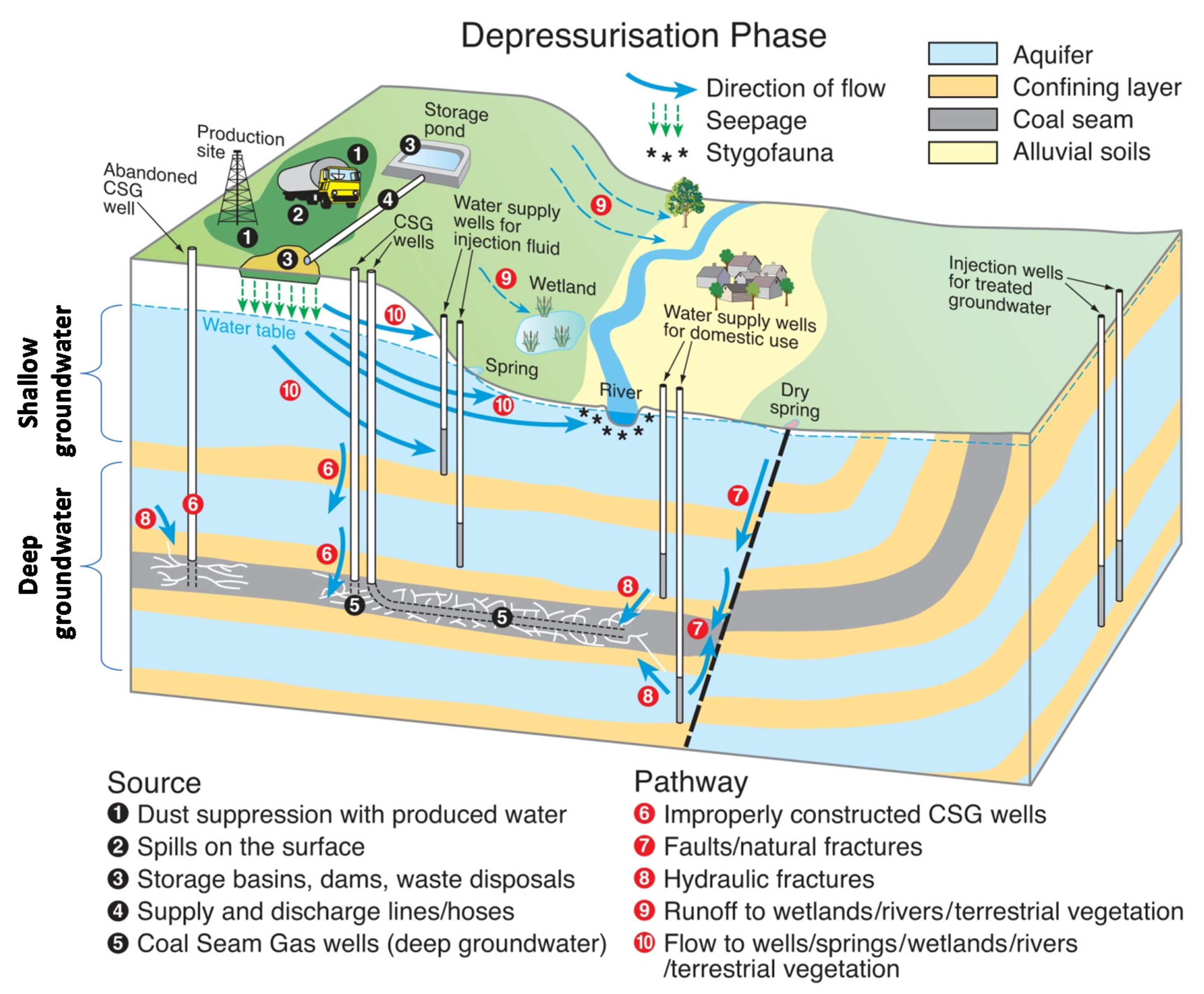
2.1. Leakage Pathways

A summary of potential leakage pathways associated with surface handling of drilling and hydraulic fracturing chemicals is available from [27]. They derived an inventory of potential scenarios of incidents involving fluid releases to soil and groundwater that is required to assess contamination risks from such surface handling activities (the assessment itself is the subject of this study). For each scenario a contamination source, migration pathway and receptor had been defined for the different phases of a typical coal seam gas project. Most reported incidents had occurred in the pre-operational phase when the well pad is prepared, including drilling and completing the well (incident probability of 0.73%) and the depressurization or gas production phase when gas is extracted and generally large volumes of produced water are transported in dedicated pipes to storage ponds and custom plants and/or treatment facilities (incident probability of 0.46%). A probability of less than one per cent is referred to as exceptionally unlikely using a calibrated uncertainty language [29]. Although the likelihood for incidents is slightly larger during the pre-operational phase compared to the depressurization phase, the focus in this study is on incidents from the latter phase (i.e., gas production phase). This is because the volume of (unlikely) fluid spills during the pre-operation phase is relatively small, easy to contain and would not normally infiltrate to great depths that would make remediation difficult.
For the gas production phase, [27] summarized multiple potential sources of chemical contamination with surface spills and leaks and multiple potential pathways and receptors for the contaminant transport of fluids associated with surface-based hydraulic fracturing operations at the CSG site (Figure 1). We report here only on the coupled soil-groundwater pathway (Pathway 10 in Figure 1) for a leaking storage pond at the land surface (Source 3 in Figure 1).
Source 3 considers infiltration from fluid holding ponds or waste disposal ponds, pond wall collapse, and hazardous events including flooding. A similar chemical migration pathway exists if pipes transporting produced water leaked (Source 4 in Figure 1). Even when appropriately designed and installed, lined ponds are known to cause small leaks over time [33,34,35,36]. Moreover, when highly saline fluids are stored, the permeability of clay lined ponds will increase [37,38]. Additionally, it has been shown that organic compounds—even when dissolved in aqueous solutions—permeate much faster through geomembranes than water [35].
Lining systems can vary considerably in complexity. The simplest lining systems consist of a compacted clay liner (CCL), a geosynthetic clay liner (GCL), or a geomembrane (GM) liner overlain by a granular drainage collection layer. A more sophisticated and effective lining system incorporates a composite liner comprised of a GM placed directly on top of a clay liner (or other type of soil liner). The most effective design considers a double composite liner with a leak detector and/or leachate collection system. The advantage of GCLs over traditional clay liners is that they are easy to install, have a low hydraulic conductivity and they have the ability to self-repair holes upon contact with leachate water, caused by the swelling and self-healing bentonite. Current engineering practices for lining landfills and storage ponds consider double liner systems which incorporate leakage collection systems. While generally low, leakage (the combination of advective and diffusive migration of chemicals) from a composite liner (GM combined with either a CCL or a GCL) cannot be avoided and is mainly due to the fact that a GM installed as part of liner system will generally have some holes [36,39,40].
Leakage rates compiled from waste containment systems range from 5 × 10⁻¹³ m/s (0.016 mm/year) to 5 × 10⁻⁹ m/s (158 mm/year) depending on the type of liner [41]. Any selection of a leak rate for solute transport calculations should represent normal operations of the storage pond, i.e., a performance that is at least as good as the design specifications and possibly better. The selected leak rate has to account for additional factors, including the variation in liner designs across the Australian landscape, the uncertainty about the leak rate for a specific liner design, and the advances in installation quality and construction quality assurance practices, yielding better performing liners. Therefore, a range of leak rates is considered rather than a single “best estimate” leak rate. Three leak rates are selected here for solute transport calculations: 0.35, 3.5, and 35 mm/year. The range 0.35 to 35 mm/year corresponds approximately with the range of leakage rates compiled for an extensive dataset of landfill liner systems [42]. The 0.35 mm/year (~10−11 m/s) could be considered a reference value for designs that include a GM/GCL composite liner. The 35 mm/year (~10−9 m/s) is considered typical for a design with a single GM liner, or a compacted clay liner if sufficiently thick.
These three classes of leakage rates assume a single liner system (i.e., a single composite liner); in case of a double liner system, the leak rates can be expected to be even lower. In addition, it is further important to note that the three classes of leak rates selected here represent a very slow, diffuse, but long-term leakage rate across the entire pond under normal operation. This is different from considering an accidental leak, in which case much higher fluid rates exist. From a preliminary assessment of a real breach in a pond liner presented in [43], it is demonstrated that much higher leak rates exist than the 10−10 m/s considered here. However, such high leak rates usually occur only over a limited surface area of the pond and the loss of considerable volumes of water generally leads to timely detection and subsequent remediation.
Pathway 10 considers subsurface flow from surface sources into the unsaturated soil/rock, potentially leaching into groundwater and further migration to water supply bores, recharge springs and groundwater-fed wetlands, and rivers. The other surface-based sources (including incidental spills) were found to be contained within the unsaturated zone [43]. For modelling subsurface contaminant sources involving drilling and/or hydraulic fracturing fluids, alternative modelling approaches have been developed [44].

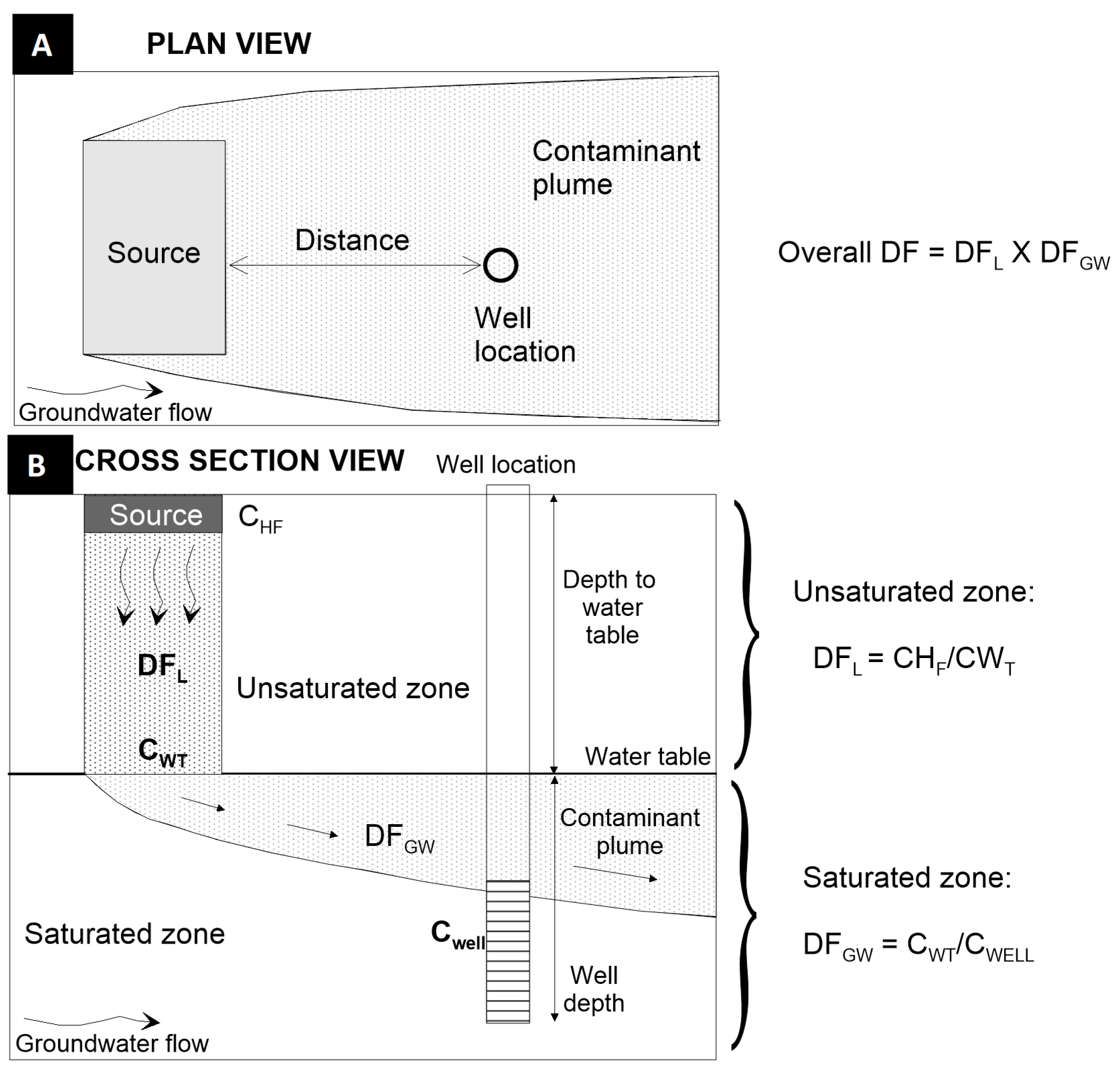
2.2. Soil-Groundwater Pathway Coupling

Although conceptually, the soil and groundwater pathway are coupled, in the calculations they will be uncoupled, i.e., into a separate soil pathway calculation and a groundwater pathway calculation. The combined effect of both pathways on solute dilution will be obtained by combining the dilution calculated for the separate pathways (Figure 2). This is done as follows: first the dilution factor is calculated at the soil/groundwater interface, then the dilution factor in groundwater is calculated separately. The soil and groundwater pathway will be discussed in detail in Section 2.3 and Section 2.4, respectively. The two dilution factors are then combined to give the overall dilution (see Section 2.5).

2.3. Soil Pathway

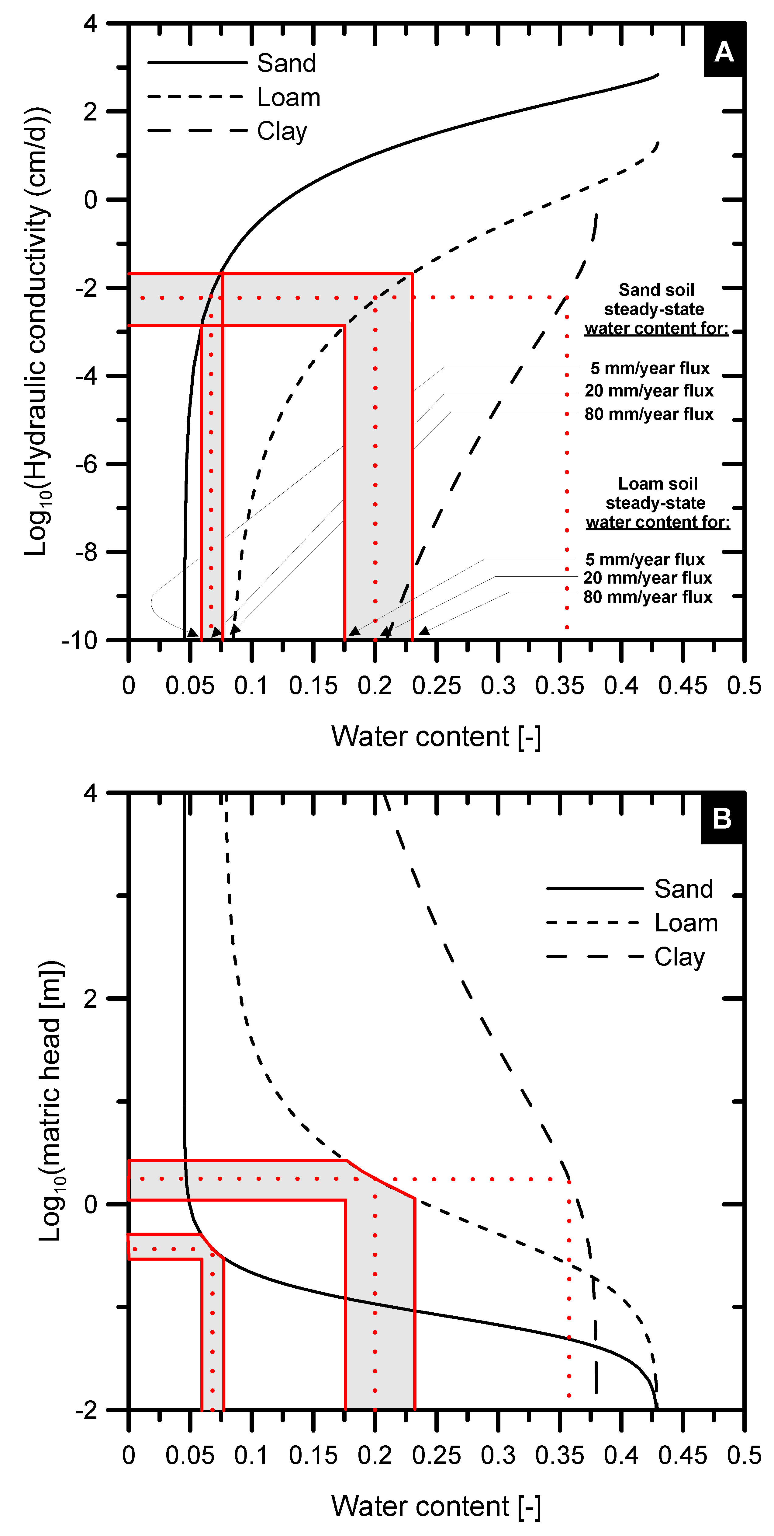
2.3.1. Soil Hydraulic Model

Simulation of variably-saturated flow in soil requires a mathematical relationship between (i) the soil water content (θ) and the soil pressure head (h), i.e., the soil water retention curve θ (h), and (ii) either the water content or the pressure head and the unsaturated hydraulic conductivity K(θ) and K(h), respectively. We applied the analytical model of van Genuchten to describe the soil water retention curve, θ (h) [46], since it permits a relatively good description of θ (h) for many soils using only a limited number of parameters. The van Genuchten soil moisture retention characteristic is defined as:
θ ( h ) = θ r + ( θ s θ r ) ( 1 + | α h | n ) m
where θr is the residual water content (cm3/cm3), θs is the saturated water content (cm3/cm3), and α (1/cm), n (dimensionless), and m = 1 − 1/n (dimensionless) are the retention curve shape parameters. The van Genuchten θ (h) equation has the additional advantage that when coupled with the unsaturated hydraulic conductivity K(h) model of [46], it produces the following closed-form expression:
K ( h ) = K s S e l [ 1 ( 1 S e 1 m ) m ] 2
where Ks is the saturated hydraulic conductivity (cm/day), Se = (θθr)/(θsθr) is the effective saturation (dimensionless), and n and m are as defined previously. The pore-connectivity parameter (l) was estimated by [47] to be about 0.5 as an average for many soils. In this study, we use Equation (2) with the l parameter fixed at 0.5.

2.3.2. Solute Transport Model

Migration of chemicals in soil is primarily by advection (transport as a result of flowing water) and hydrodynamic dispersion (transport as a result of mechanical dispersion and molecular diffusion) (ignoring gaseous transport) [48]. Simulations for the transport of contaminants during steady-state or transient water flow were undertaken with the one-dimensional HYDRUS-1D simulator [49,50]. The use of a one-dimensional model is justified because leaching processes over short or longer depths are typically one-dimensional in flat areas where lateral subsurface flows are negligible. A two-dimensional approach may be more appropriate when soil layers with a sloping interface are present, which may exist on hillslopes [51]. However, given the very flat topography of the study region, lateral flows are not expected.
Solute advection is determined by the pore-water velocity v, which is defined by the soil water flux q and the soil water content θ, i.e., v = q/θ. For transport of inert, non-adsorbing contaminants during transient water flow the advection-dispersion equation is as follows [49]:
θ c t = z ( θ D 2 c z 2 ) q c z
where c is the solute concentration in the water phase (mg/L), t is time (d), D is the hydrodynamic dispersion (m2/day), z is the soil depth (m), q is the soil water flux (m/d), and θ is the soil water content (cm3/cm3). Hydrodynamic dispersion is the sum of molecular diffusion (very small relative to advection) and mechanical dispersion (governed by the longitudinal dispersivity AL (m)). The approach adopted here for solute transport through unsaturated soil assumes an asymptotic longitudinal dispersivity AL is reached after a transport distance of 5 m with a corresponding dispersivity AL = 0.1 m. This is based on the review of dispersivities for soils, where for field tracer tests the 75th percentile of dispersivity values was 0.1 m for both coarse and fine textured soil [52]. We choose this dispersivity value from field tests that excluded ponding conditions and with flow velocities less than 10 cm/day. These conditions are the most representative of our study, where the reference water flux for recharge is 20 mm/year (or 0.0055 cm/day) and the reference leak rate is 0.35 mm/year (0.000096 cm/day). For our long-term simulations, the dispersivity is kept constant during the simulations as the long-term water profile is at steady-state, except for a short period when the recharge rate from the warming-up period changes to the leak rate and then back to long-term recharge. For transport distances from 0 to 5 m, a linear increase in dispersivity has been assumed here (i.e., at x = 1 m, AL = 0.02 m; at x = 2 m, AL = 0.04 m; at x = 3 m, AL = 0.06 m; at x = 4 m, AL = 0.08 m; and at x = 5 m, AL = 0.1 m). For transport distances from 5 to 30 m a constant value of AL = 0.1 m is adopted. Such low values better reflect the observed dispersivities for steady-state unsaturated flow in soil [52].
The only physical transport processes accounted for in the current assessment are advection and hydrodynamic dispersion. Together with the dilution or the mixing of dissolved chemicals with uncontaminated soil water, these are thus the only attenuation processes that result in reducing the contaminant concentration while vertically migrating through the unsaturated zone. In other words, our conservative transport calculations do not account for chemical interactions between contaminants and the solid phases (e.g., clay minerals, organic matter, metal oxides, and hydroxides) and further ignore biogeochemical transformations [53] that would otherwise further reduce solute concentrations [4].
An important parameter determining solute transport calculations through soil is recharge: the fraction of infiltration water that reaches the water table [48]. In other words, the rate of percolation water arriving at the groundwater table. This value was used as an upper boundary condition for the solute transport modelling, and was assumed constant throughout the soil profile. The current approach simplifies typical water balance calculations by imposing previously determined groundwater recharge rates on the solute transport model (i.e., q = recharge rate in Equation (3)). Recharge was thus not calculated here by applying mass balance principles but instead was taken from previous studies (for details, see below and [43]); given the uncertainty about this parameter, uncertainty bounds were imposed on recharge in this study. Furthermore, different soil materials (fine textured, coarse textured, and their mixtures) will result in different hydraulic conductivity and water content profiles in the unsaturated zone for any given recharge rate (see e.g., [46]). For the same water flux at the soil surface, such differences in water content will also result in different solute transport velocities. To account for this effect on solute dilution, different soil hydraulic properties were implemented (see further).
This approach is a simplification of the true infiltration process, where under dry conditions the infiltrating water at the soil surface may fill up pore space, with water being subsequently lost via evapotranspiration, while under near-saturated conditions all the infiltrating water may reach the groundwater table. However, for long-term simulations such as ours, these short-term transient processes average out and can be replaced by a steady-state flux. Note that the model still has a transient period when the water flux changes from a given leak rate (reference value of 0.35 mm/year) to a given recharge rate (reference value of 20 mm/year), after the water holding pond has been dismantled and natural recharge takes over.
Average groundwater rainfall recharge in the case study area (Namoi catchment, New South Wales) was found to range from 5 to 70 mm/year [54,55,56]. Because our study area falls within the areas of reported recharge values, and has similar soil coverage and hydrogeology, the reported values were considered representative. Based on these literature values, a best estimate of 20 mm/year recharge for the study area was selected. To account for variability in the recharge values, model simulations consider three values: a best estimate (BE) of 20 mm/year, a minimum value of 5 mm/year (BE/4), and a maximum of 80 mm/year (BE × 4). The minimum and maximum were considered suitable to capture the range of reported recharge values.
These recharge values were obtained through numerical modelling using different models with different spatial and temporal domains. For the Upper Namoi Groundwater Model (2500 km2), recharge was model-calibrated for the period 1985–2002 [54]. For the Liverpool Plains, the catchment model SWAT (437 km2) was used to calculate long-term average recharge for the period 1957–2000 [55]. Diffuse recharge for Lake Goran (1550 km2) was derived from various modelling studies [56].
Dominant soil groups within the case study area of the Namoi alluvium are grey, brown, and red clays and black earths, commonly known as Vertosols (Table S1). Despite their high clay content (at least 35% field-based clay content for the Vertosols), the grey, brown, and red clays have a relatively high infiltration capacity as a result of cracking clay throughout the soil profile [57]. However, such preferential flow features are typically of short duration as the cracks close upon wetting which reduces considerably soil infiltration capacity. Furthermore, the effect of cracks would be most noticeable under conditions of surface irrigation (furrow), but much less so for natural rainfall conditions when surface saturation is less common. Soils with a predominantly sandy texture include lithosols, non-calcic brown soils, and earthy sands. While any of the Great Soil Groups is highly variable in terms of texture class, such textural information was not provided with the available digital soil map. We have therefore taken two contrasting texture classes (i.e., sand and loam) that were assumed to provide a realistic though simplified representation of the natural variation in water contents, hydraulic conductivity, and hence solute velocities for the defined recharge rates. Based on the distribution of soil groups in Table S1, a loam textured soil would be representative for most of the mapped soils (92% based on Vertosols and Chromosols Orders), whereas a sand textured would represent only a small fraction of the soils (8% based on Sodosols and Other Orders). The results obtained with the loam soil are therefore considered as a reference, recognizing however, that the unsaturated sediments underlying the soil may have a different texture and structure and thus different hydraulic properties.
Because soil hydraulic properties for each of the different soil groups were not available at the time of the assessment, the soil hydraulic properties for the analytical functions of van Genuchten-Mualem (Equations (1) and (2)) associated with the loam and sand soil were taken from [58]. The loam and sand textures considered by [58] represent two out of the 12 textural classes of the United States Department of Agriculture (USDA) soil textural triangle [59]. A similar data base with soil hydraulic properties is not available for Australian soils. For the purpose of calculating a broad range of unsaturated zone flow conditions, the use of the Carsel and Parrish hydraulic properties was deemed justified. As can be seen from the unsaturated hydraulic conductivity and soil water retention characteristics in Figure 3, the sand and loam soils represent a fairly broad range of hydraulic conditions in unsaturated soil for the selected range of recharge rates (at the groundwater table).
The grey-shaded area in Figure 3 represents the variation in soil water content conditioned by the range in water fluxes (i.e., recharge rates), and thus is a measure of the variation in solute velocity, which has been considered in the solute transport calculations. The imposed variation in water fluxes at the soil surface (i.e., from 5 to 80 mm/year) results in a larger range of steady-state soil water contents for the loam (i.e., from 0.175 to 0.23 cm3/cm3) than for the sand textural class (i.e., from 0.059 to 0.074 cm3/cm3). For the relevant water fluxes (i.e., recharge rates) considered in this study (from 5 to 80 mm/year), the clay textural class would result in the highest steady-state water content of approximately 0.35 cm3/cm3. Because solute velocity is inversely related to soil water content (v = q/θ), solute leaching will be slowest in clay and fastest in sand. In other words, a study that considers sand, loam, and clay would have the earliest arrival of the solute plume at the groundwater table for the sand and the latest arrival for the clay soil. The loam would provide an intermediate arrival time. In the current assessment, only the soil textures providing the two earliest arrival times are considered, i.e., sand and loam. This way, high-end estimates of solute behavior—in terms of arrival time—have been derived. Given that loam type soils represent 92% of the study area, only the results for loam are reported here. The results for sand soil are available from [43].

2.3.3. Accounting for Variations in Depth to Groundwater

Depth to groundwater plays an important role in determining the contaminant concentration at the soil-groundwater interface, with greater depths providing more opportunity for attenuation by dilution, dispersion, and biogeochemical processes [4]. Depth to groundwater describes the distance from the land surface down through the unsaturated zone to the average water table depth and was used to define the domain geometry in HYDRUS-1D (vertical length or depth). This depth is mildly variable in our case study area, as is evident from the water table map for the Narrabri Alluvial aquifer (see Figure S1 and [60]). The depth to shallow groundwater was determined from groundwater level measurements available in the National Groundwater Information System (NGIS) database (Bureau of Meteorology); depths vary from 1.7 to 24 m for the sub-regional (or local) groundwater model domain (Figure S1). The average depth to the shallow water table for the entire sub-regional model domain is 21.3 m, based on a model domain of 108 km2 with grid cells of 1 × 1 km2. This study assumes a long-term average groundwater level without any increase or decrease in groundwater level due to external factors (such as seasonal climate, climate change, coal seam gas extraction, mining, agricultural extraction, etc.).
Spatial distributions of depth to groundwater for both the site groundwater model (which covers a surface area of 24 km2) and sub-regional groundwater model (108 km2) are provided in Tables S2 and S3, respectively. Based on the site model, most soils in the Namoi Alluvium have depths to groundwater in the range 0 to 5 m (Figure S1 and Table S2). For the sub-regional model, most soils have a relatively shallow water table with approximately 66% of the area in the 0 to 5 m depth range. For approximately 20% of the area, depth to groundwater is up to 30 m and more (Table S3).
Although unsaturated zones with depths to groundwater beyond 10 m do not seem to occur in the relatively small site groundwater flow model domain (Figure S1, Table S2), depth to groundwater was extended in the soil model domain up to 30 m to also account for deeper soils determined from the larger sub-regional model (Table S3). In other words, the soil model domain depth varies to match the varying depth to groundwater across the larger study domain. Due to the lack of deep unsaturated zone soil data, a homogenous soil domain was assumed for all simulations. However, if site-specific calculations are carried out, it is recommended to collect stratigraphic information for the entire unsaturated zone for more detailed calculations.
The one-dimensional (1D) soil domain was discretized in a large number of numerical layers with layer thickness, Δz, depending on the soil depth: Δz = 0.01 m for soil depths of 1 and 2 m (i.e., all numerical layers from the soil surface down to 2 m have a thickness of 0.01 m); Δz = 0.015 m for soil depths from 3 to 4 m; Δz = 0.1 m for soil depths of 5 to 30 m. The numerical grid was implemented in the finite element code HYDRUS-1D [49].
The study has been simplified by performing solute transport calculations for the depth range 0 to 30 m, independent of the location of the source. In this way a concentration–depth (or dilution factor–depth) relationship can be established for further use. For existing coal seam gas sites, the relevant depth of the unsaturated zone can be derived from the combination of the land surface topographic level and groundwater level, followed by the derivation of the unsaturated zone dilution factor (DFL) associated with that depth (subscript L refers to leakage). The DFL can be linked to the groundwater dilution factor (DFGW) to calculate the solute concentration in a receiving water bore (Figure 2). It is also possible to produce a simplified map displaying the spatial variation in groundwater dilution factors. Such a map allows for a quick assessment of the dilution risk in different parts of the landscape, and spatial variation in groundwater concentrations for specific chemicals in relation to the proximity of receptors.
A further simplification of the domain geometry relates to the assumptions made about how soil layers have been represented in the model. This simplification is commensurate with the generic nature of this study, as the flow and solute transport simulations directly use groundwater recharge as the key soil hydrologic parameter rather than using specific soil physical properties of each layer to calculate recharge. For site specific assessments, detailed information such as soil horizons and their respective soil hydraulic properties for recharge estimation is recommended.

2.3.4. Boundary Conditions for Unsaturated Solute Transport

Boundary conditions for advective-dispersive solute transport accommodate the previously defined solute source for a leaking water holding pond (Source 3 in Figure 1) with the following hypothetical parameters: an area of 100,000 m2, leaking for 3 or 30 years [43]. Leakage calculations assume three hypothetical leak rates: a reference value of 0.35 mm/year, a 10 times higher value of 3.5 mm/year, and a high-end value of 35 mm/year (see [60] and the discussion on its derivation). These leak rates represent the leakage over the entire surface area of the pond under normal operation; the leak rates are determined by the design criteria of the liner of the water holding pond (see Section 2.1). A full discussion on all the other solute sources is available from [43]. A hypothetical unit concentration value has been used for the purpose of deriving dilution factors, travel times, fluxes, and concentrations. Since all transport processes are linear, a simple rescaling allows the results obtained from a unit concentration to be rescaled for any other concentration [60].
The conceptual model further assumes (i) a period with a constant natural recharge prior to the leak period and (ii) a period, following the ending of the leak, with the same natural recharge. The first period (‘warming-up’ period of 100 years) allows the soil profile to achieve a steady-state water content along the entire unsaturated zone profile. The period following the ending of the leak is continued until the peak concentration is reached at the bottom of the unsaturated zone profile (up to 1400 years for a 30-m-deep loam soil, see further).

2.4. Groundwater Pathway

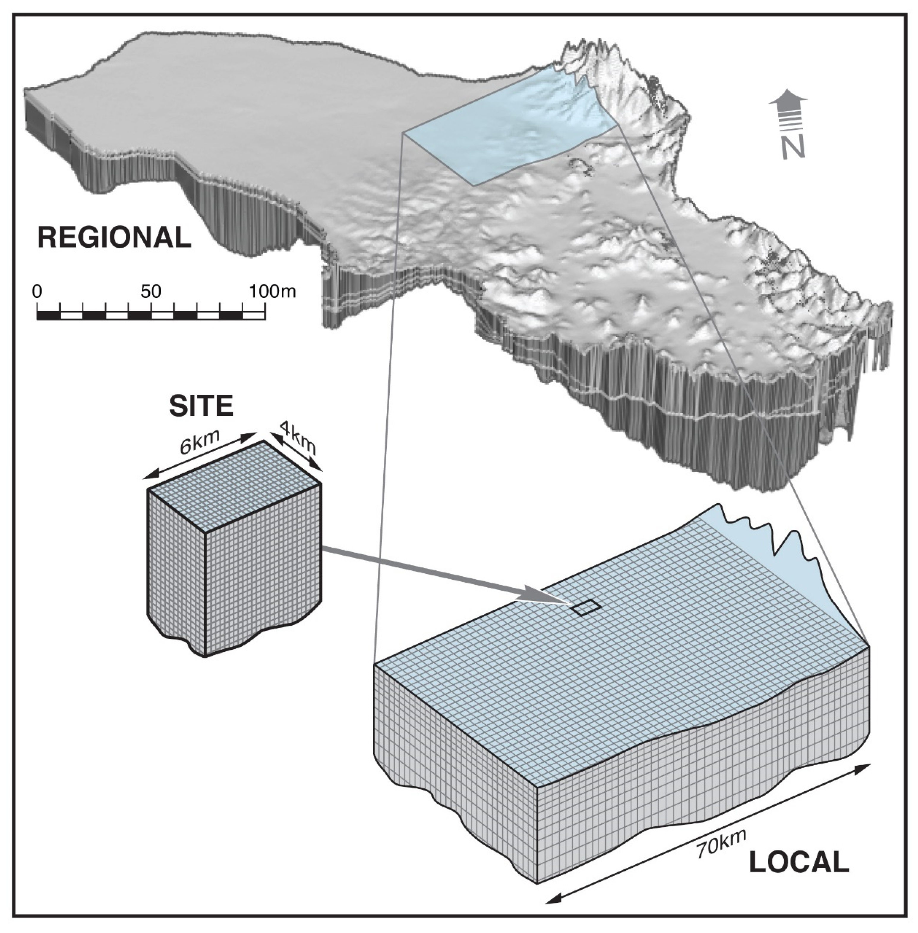
2.4.1. Groundwater Flow Model

Our case study area was a subregion within the Namoi Catchment, which straddles the boundary between the Gunnedah and Surat Sedimentary Basins (New South Wales). The three-dimensional numerical groundwater model used for this study has previously been calibrated specifically for this study area. We used the site-specific calibration as a starting point for developing more detailed small-scale flow and transport models that were used to develop generalized predicted environmental concentrations. The alluvial model components—the shallow aquifers along river channels—have been rigorously tested [61,62].
The model used a relatively coarse spatial discretization of 1 × 1 km2, which means that many of the small-scale (i.e., within-grid) heterogeneities in geological and hydrogeological properties were not effectively captured. This means that, for instance, small-scale heterogeneity in hydraulic conductivity (K) was not present in the groundwater flow model. While effects of such small-scale heterogeneity in K on groundwater flow and solute transport have been amply demonstrated in the literature [63,64,65], such effects were to some degree indirectly accounted for in this study through the use of the dispersivity parameters. As the dispersivity parameter is predominantly the result of spatial variations in pore-water velocity, variations which are driven by spatial variability in K, it determines the degree of solute mixing in groundwater and is an effective parameter that captures the average large-scale solute mixing process. This study used block-scale effective parameters to simulate solute transport. As a result, the true field-scale heterogeneity was likely underestimated. However, the main objective was to determine the maximum solute concentration, not early arrivals. The maximum concentration was less affected by heterogenous flow field compared to early solute arrival. To capture early solute arrivals, the hydraulic conductivity of the aquifer was varied over a reasonable parameter range. In this way, early, mean, and late arrivals could be captured (see further).
Furthermore, the 1 × 1 km2 grid cells of the 108 km2 large sub-regional groundwater model would not be able to represent contaminant sources, large concentration gradients, and receiving environments at a sufficiently detailed spatial resolution; it would also not be suitable for solute transport calculations where small grid cells are a pre-requisite for reducing numerical dispersion and oscillations. A finer discretization offers the additional advantages of enabling the user to accurately delineate the contaminant source area and the target receiving environments, while minimizing numerical dispersion and oscillations [66]. The local grid refinement technique [67] was used in this study, with a site model being developed from the existing groundwater model (see Figure 4). The refinement resulted in a 24 km2 site model with 50 × 50 m2 grid cells designed for solute transport simulations.

2.4.2. Solute Transport Modelling

For the purpose of solute transport simulations, the groundwater flow simulations carried out with MODFLOW were used to provide the three-dimensional velocity fields to run the solute transport model in MT3DMS [68]. A spatially uniform reference value for effective porosity (ƞe) of 0.2 cm3/cm3 for all stratigraphic units was used to obtain pore-water velocities (v) from groundwater fluxes (q): v = q/ƞe (note: as discussed above, in soils, ƞe was replaced by soil water θ). The three-dimensional advection dispersion model assumed a longitudinal dispersivity AL of 5 m, and a horizontal (ATH) and vertical (ATV) transverse dispersivity of 0.5 and 0.05 m, respectively. The value of 5 m for longitudinal dispersivity (AL) was based on the literature review by Gelhar et al. [69] where for a transport distance between 100–1000 m the average dispersivity is about 5 m. The transport distance 100–1000 m is appropriate for this study where observation points range from 100 to 2000 m (see further). For the horizontal (ATH) and vertical (ATV) transverse dispersivity, the value of AL was divided by 10 and 100, respectively, consistent with [70].
The solute transport model considered a chemical source in 40 cells, 50 × 50 m2 each, or a total source area of 100,000 m2 (0.1 km2 or 10 ha) (Figure 5). The source area is in the center of the model and corresponds to the location of a hypothetical water holding pond with fluids leaking into the subsurface at very slow rates; at the soil-groundwater interface, a solute flux with a unit concentration of 1 mg/L and a reference water flux of 20 mm/year was assumed. The latter water flux corresponds to the reference long-term average recharge rate and was used to produce a solute flux (solute flux = water flux × solute concentration) from the soil into the groundwater. The recharge rate rather than the leak rate was used to describe the solute flux into the groundwater because for the deeper soil depths, the solute does not reach the soil-groundwater interface during the three-year leak period [43]. The solute reaches the interface as a result of infiltrating rainwater (i.e., recharge) pushing the solute plume further down; hence, the solute will reach the groundwater at a rate mainly defined by the recharge and less so by the leak rate.
Solute fluxes at the soil-groundwater interface have been calculated with the HYDRUS-1D simulator for a total of 96 parameter combinations (2 soil types × 3 recharge rates × 2 leakage rates × 8 soil depths = 96 combinations). Rather than applying each of these different solute flux predictions separately to the groundwater transport model, a simplification was introduced by assuming a hypothetical unit concentration source (1 mg/L) at the top of the aquifer. This concentration was then multiplied with the recharge rate to obtain a solute flux entering the aquifer. This solute flux in the 0.1 km2 (10 ha) source area was kept at a constant value for a time long enough for the concentration at the different water bores to reach a steady-state value. This approach of uncoupling the soil and groundwater solute transport calculations is consistent with Figure 2, which shows that the dilution factors for the soil-groundwater pathway were split in two components: first, the dilution factor was calculated at the soil/groundwater interface, then, the dilution factor in groundwater was calculated separately. The two dilution factors were then combined to give the overall dilution as per Equation (6). This way, the calculations were made highly efficient such that many realizations could be tested as part of the uncertainty analysis.
Consistent with the need to derive high-end estimates, the assumption of a continuous input function results in an overestimation of the solute concentration for cases where the solute flux at the soil-groundwater interface is a narrow, short-duration pulse. This method also avoids running the solute transport model multiple times to account for the different input functions originating from the solute transport calculations in soil (i.e., 96 input functions are replaced by a single one with constant solute flux).
Solute concentrations were recorded at hypothetical water bores located at increasing distances from the source, i.e., at 100, 200, 400, 800 and 2000 m (Figure 5). The location of the bores coincides with the center of the solute plume for most of the calculation cases; in this way, maximum concentrations were used to derive dilution factors. Exceptions existed for cases where the solute plume was diverted along a more curved path westward towards the river owing to changes in the hydraulic gradient consistent with the decrease in aquifer hydraulic conductivity by a factor of 5 and increases in riverbed conductance by a factor of 7. The location of water bores was not adjusted to keep the same water bores for calculating and comparing dilution factors across different scenarios.
The water bores were assumed to be screened over their entire 50-m depth. Depth-weighted mean concentrations are obtained for all bores: C = ΣCi × Zi/Ztotal, where Ci is the concentration in layer i (with i = child model layers 2, 3, and 4 of the Gunnedah Formation), Zi is the depth of layer i, and Ztotal is the total depth (i.e., 50 m). While water bores are typically sunk to different depths, the highest solute concentrations are likely to be closest to the water table, therefore justifying the consideration of shallow depths only (i.e., up to 50 m). Furthermore, considerable mixing of groundwater—and thus also solutes—from different layers occurs while pumping. It is thus justified to assume a depth-averaged concentration to represent this mixing process.
The groundwater flow calculations further included three perturbations of hydraulic conductivity (low K = reference K/5, reference K, high K = reference K × 5) and of riverbed conductance, respectively (low = reference river conductance/7, reference river conductance, high = reference river conductance × 7), thus producing nine groundwater flow scenarios for subsequent transport calculations. Changing hydraulic conductivity and riverbed conductance resulted in changes to the groundwater gradient and surface water–groundwater flux. The solute transport simulations further considered perturbations of the effective porosity, again with three values: 0.10, 0.20 (reference), and 0.40 cm3/cm3. This range in porosity corresponded to the range of reported vales from 0.15 to 0.39 [60], with 0.2 selected here as a reference value. As a result, 27 solute transport simulations were carried out with the site model. While this number of parameter perturbations was smaller than what is typically used in a full-scale Monte Carlo analysis (typically several hundred or thousand runs to achieve convergent statistics), it nevertheless provides a reasonable range of parameter variations while at the same time being very efficient in terms of computational resources. Moreover, note that the perturbations were applied uniformly throughout the groundwater model domain.
Solute transport calculations were carried out using the Implicit Finite Difference solution scheme with upstream weighting to calculate advection [71]. Among the finite difference schemes in MT3DMS (explicit and implicit finite difference (FD), third order Total Variation Diminishing (TVD)), this scheme is the most stable, is computationally efficient, often gives the best mass balance (i.e., it is mass conservative), and is also less computationally demanding than a TVD solver [71].
An important path to achieving confidence in model simulations is to perform the numerical simulations in a way that is consistent with established principles and guidelines. As far as groundwater modelling is concerned, the Australian groundwater modelling guidelines [72] provide a point of reference for groundwater flow and transport calculations. In the current exposure assessment, the Australian groundwater modelling guidelines have been used as a guide for groundwater flow and transport calculations.

2.5. Dilution Factors

Dilution of chemicals occurs both in the unsaturated soil zone and in groundwater. A dilution factor is therefore defined for the unsaturated zone (DFL) and groundwater (DFGW), where DFL is the ratio of contaminant concentration in the fluid (hydraulic fracturing-related or produced water) leaked at the surface (CHF) to the maximum contaminant concentration at the bottom of the unsaturated zone, i.e., at the water table (CWT): DFL = CHF/CWT (Figure 2). The calculation of DFL typically involves a one-dimensional solute transport model for the unsaturated zone. The DFGW is calculated as the ratio of the maximum contaminant concentration at the bottom of the unsaturated zone (CWT) to the maximum concentration at the water bore (CWB): DFGW = CWT/CWB. The combined dilution in unsaturated zone and groundwater (DF) is defined as:
D F = D F L × D F G W
All dilution factors thus defined are dimensionless, and larger than one. This approach is consistent with that applied by [60].
The dilution factor for soil is mainly determined by the soil type and depth, recharge rate, and leak rate from a storage pond. Calculations that neglect chemical interactions with soil materials will considerably overestimate the consequences and therefore deliver conservative risk assessments. If it can be shown that under such conservative assumptions the impact is negligible, impacts under more realistic conditions with considerable degradation and sorption will be even smaller. The degree of overestimation or conservatism will be less for calculations that account for chemical interactions or biogeochemical transformations. In such case, dilution (or attenuation) can be shown to be very sensitive to such reactions resulting in considerable decreases in concentration [4].
For the dilution factors (and other computational endpoints) to be broadly applicable, i.e., covering a sufficiently broad range of soil and groundwater flow conditions, multiple calculations of such dilution factors have been undertaken with different soil and groundwater parameters that govern solute migration.
Once the dilution factors for the various receiving environments have been defined, the concentration at the water table (CWT) or at the water bore (CWB) for any concentration of a specific chemical at the surface (CHF) can be calculated. Calculation of CWT and CGW is as follows:
C   W T = C   H F D F L
C WB = C WT D F GW = C HF ( D F GW × D F L )
The calculation of dilution factors must be done only once for a given source-pathway-receptor combination. Further note that the linkage between soil and groundwater pathway is provided via coupling (i.e., multiplication) of their respective dilution factors. The combined dilution (DF) from travelling through the unsaturated soil (DFL) and subsequently through groundwater (DFGW) was calculated as the product of the dilution associated with each system separately (see Equation (6)). This assumes that transport and hence dilution occurred independently in both pathways. This was true for most circumstances: transport in soil (especially deep soils) occurred independently from groundwater flow. Only in shallow soil with large groundwater level fluctuations can solute migration be significantly influenced. Therefore, once recharge was accounted for, transport in groundwater was considered independently from all other soil processes.

3. Results

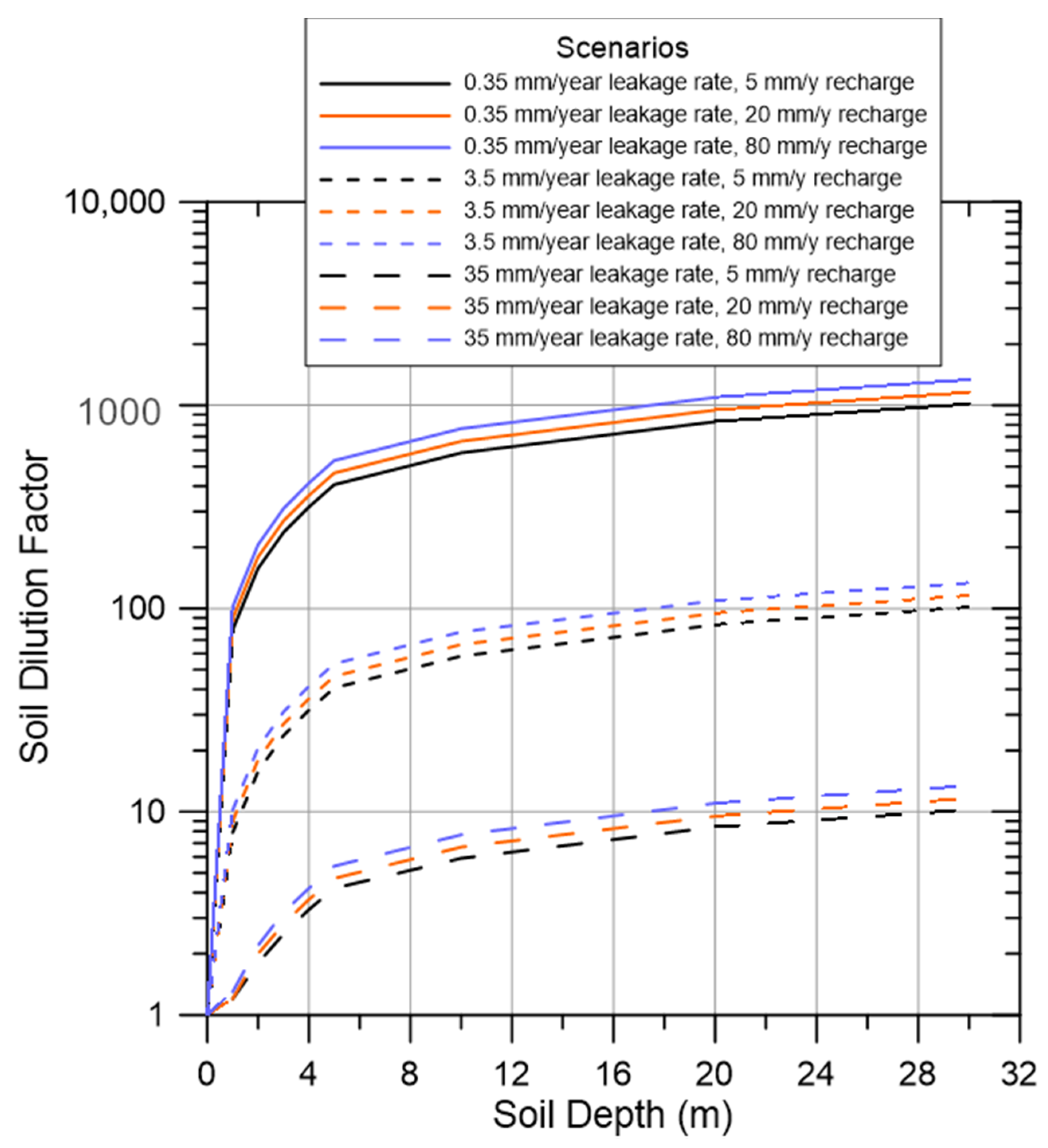
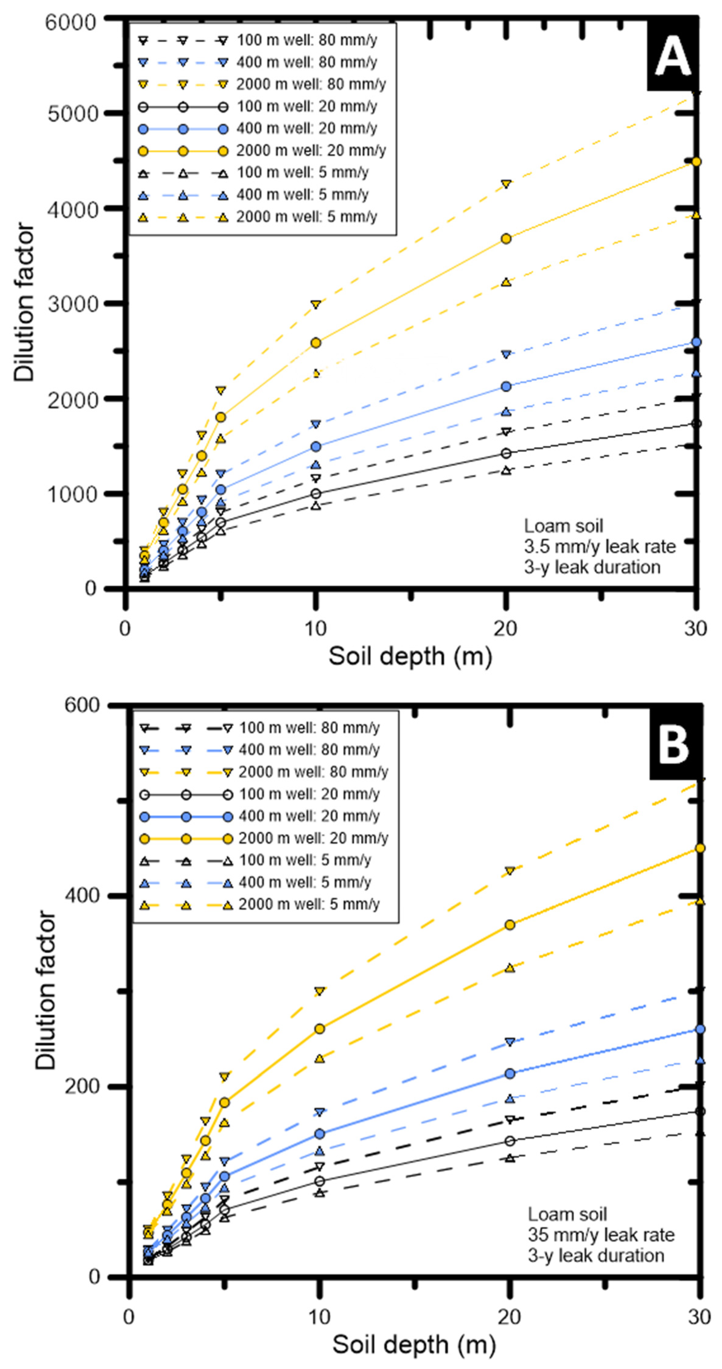
3.1. Soil Dilution Factors

The time for solutes to travel from the source to the bottom of the soil profile (soil–groundwater interface) is discussed first. As mentioned above, these are conservative arrival times without considering the retardation effect due to sorption. Additional solute retardation due to chemical-solid interactions can be easily a factor 100 to 1000 based on previous assessments [4].
Solute transport in the loam soil was slower than the sand due to the lower pore-water velocity (v = 0.1 mm/year for the loam and 0.3 mm/year for the sand); earliest arrival in the loam soil was after 12 years for the 1-m-deep soil and 40 years for the 4-m-deep soil (for a three-year leak duration, reference leak rate of 0.35 mm/year and 20 mm/year recharge). For the sand soil the earliest arrival was after six years for the 1-m-deep soil (same conditions as for the loam soil) and 15 years for the 4-m-deep soil (same leak rate).
For the 5- to 30-m-deep soils, the results are as follows. The earliest arrival for the loam soil was after 50 years for the 5-m-deep soil (for the reference leak rate of 0.35 mm/year and 20 mm/year recharge) and 300 years for the 30-m-deep soil (same leak rate and recharge rate). Solute transport in the sand soil was faster due to the higher pore-water velocity; the earliest arrival was after 19 years for the 5-m-deep soil (for the reference leak rate of 0.35 mm/year and 20 mm/year recharge) and 100 years for the 30-m-deep soil (same leak rate and recharge rate).
Vertical profiles of solute concentration and water content during and after the leak event provide an insight in the dynamics of coupled water and solute transport (Figure S2). The solute concentration profiles at different times displayed a characteristic bell-shaped behavior, as was expected for a leak event of a relatively short duration. As time progresses and the solutes move down, the shape of the curve widens and the maximum concentration decreases owing to dispersion. The time-dependent water content profile displays a draining soil the first three years, then a wetting profile until equilibrium is again achieved. Drainage occurs because the leak rate (0.35 mm/year) is considerably less than the initial recharge rate (20 mm/year); after the leak event, the water flux becomes again equal to the recharge rate (20 mm/year), effectively wetting up the soil profile until the water content becomes equal again to its initial value.
Dilution factors as a function of soil depth for a three-year leak are shown in Figure 6 for the loam soil and account for uncertainty in the leak rate and recharge rate. A 10-fold increase in leak rate decreases the dilution factors by a factor of 10. The overall uncertainty is attributable mainly to the leak rate and less so to the recharge rate. As the depth increases, dilution factors also increase; however, the rate of increase decreases quickly beyond the 5 m soil depth due to the dispersivity parameter becoming constant at 5 m (AL = 0.1 m).
For loam soil, the range in dilution factors at 1 m depth due to uncertainty in the recharge rate was from 79 (89% of the reference value) to 102 (115% of the reference value); at 30 m depth the range was from 1013 (87% of the reference value) to 1334 (115% of the reference value). For sand, the range in dilution factors at 1 m depth was from 26.5 (91%) to 33.1 (113%); at 30 m depth the range was from 340 (91%) to 426 (114%). Dilution in loam was roughly three times larger than in sand, irrespective of depth. This is due to the three times higher water content in loam compared to sand; under those conditions, chemicals entering a loam soil will be three times stronger mixed with solute-free water compared to sand.
When a leak duration of three years is considered, the solute travel time to a given depth is insensitive to the magnitude of the leak rate. This is because the leak duration is short relative to the duration of solute migration, i.e., the latter is close to 200 years if the groundwater table is at 10 m. Under such conditions, the travel time is predominantly determined by the water flux (i.e., recharge rate) following the leak event. Unlike the travel time, the maximum solute concentration at any depth is significantly affected by the leak rate: a 10-fold increase in the leak rate increases the maximum concentration by about a factor of 10. With the higher leak rate more solute mass enters the soil profile which becomes less easily diluted when solute-free water enters the soil after the leak has stopped. Dilution factors for a 30-year leak rate are 10 times smaller for all parameter combinations (for details, see [43].
It is important to emphasize that the above results have been obtained using a 1D flow and transport model that does not consider preferential flow. Increasing evidence exists that water in many soils does not move according to the uniform flow pattern typically predicted with the Richards equation [73,74,75]. This is due to the presence of macropores, fractures or other structural voids or biological channels through which water and contaminants may move preferentially, while bypassing a large part of the matrix pore-space. Preferential flow and transport processes limit accurate predictions of contaminant transport in soils and fractured rocks [76]. While several studies have indicated the importance of preferential flow on solute transport in soil, little evidence is available about the significance of such processes for the soils and sediments considered here, although catchment-scale water balance modelling involving cracking soils in the Liverpool Plains (New South Wales) was considered by [55]. It is important to note though that preferential flow via macropores, fractures and similar soil structural features becomes important when the flow regime is close to saturation (i.e., when the macropores are filled with water and effectively contribute to flow and transport). Under the flow conditions of this study, i.e., soil conditions that are far from saturated, preferential flow is likely less important. Nevertheless, it remains an important uncertainty that requires further corroboration.

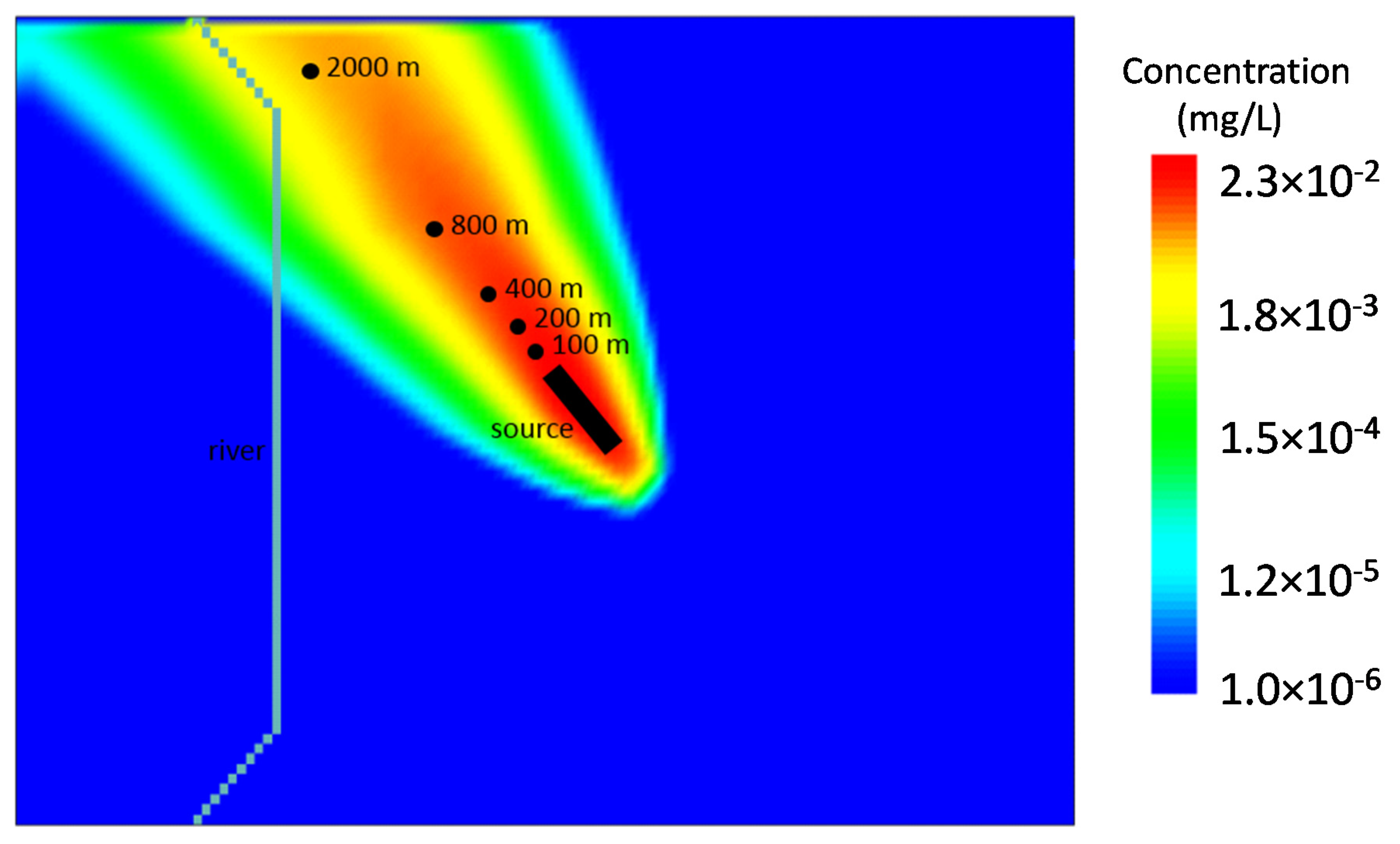
3.2. Groundwater Dilution Factors

Development of the solute plume for the reference scenario based on the reference groundwater flow model with spatially uniform effective porosity (ƞe) of 0.2 cm3/cm3 and a continuous input function is shown in Figure 5. The water bores are located along the center of the solute plume and record the maximum concentration for the purpose of calculating dilution factors. Note the long simulation times applied to all scenarios to ensure the maximum concentration was reached in each of the observation bores. The travel time to the water bores at 100 and 800 m distance is 62 and 180 years, respectively. Solute arrival times were calculated as the time needed for the solute to travel through groundwater and reach one half of its maximum concentration at a particular water bore; half the maximum concentration was chosen as a reference point in time for calculating the arrival time, as this would be the time the continuous pulse would reach the water bore in absence of dispersion [77]. The advantage of this approach is that it made the determination of solute arrival times independent from the hydrodynamic dispersion, a process that is highly variable in space.
The reference scenario represents the realistic high-end scenario (i.e., a scenario that captures the upper end of the exposure distribution for a given exposure pathway [78]), while the other 26 scenarios represent the results for a realistic range of parameters typical of the investigation area. With a total of 27 parameter combinations, a total of 27 breakthrough curves (BTCs) have been calculated for each water bore.
Dilution factors for the groundwater receiving environments (water bores) have been calculated in the same way as for the soil pathway. Dilution increases in a nearly linear way with increasing distance, i.e., at 200, 400, 800, and 2000 m dilution is on average, respectively, 1.2, 1.5, 2.1, and 4.1 times larger than at 100 m (Table 1). An exception exists for the low aquifer conductivity–high riverbed conductance and reference aquifer conductivity–high riverbed conductance parameter combination: under these conditions, the direction of the plume is different, i.e., bending towards the river and less to the north-west. As a result, the center of the plume diverges from the observation bores at large distance (800 and 2000 m), which explains the lower maximum concentrations and hence larger dilution factors. Dilution factors at 2000 m were not calculated for those parameter combinations because the center of the plume completely bypasses the bores at 2000 m; this would produce artificially high dilution factors.
Although three porosities were used (0.1, 0.2, and 0.4 cm3/cm3) for any given aquifer conductivity–riverbed conductance combination, identical dilution factors have been obtained. This was, as expected: increasing (here by a factor of 2) or decreasing (also by a factor 2) porosity compared to the reference value results in higher (2 times) and lower (2 times) pore volumes in which the solutes were dissolved. The resulting concentrations were, respectively, lower by a factor of 2 and higher by a factor of 2. However, just underneath the source zone, there was a counteracting effect of the pore-water velocity in groundwater. Indeed, a two-time higher porosity resulted in a two-time lower pore–water velocity under the source zone: as a result, more mass will be taken up in a volume of groundwater per unit of time (exactly two times more), and thus, more mass can be transported away from the source. At the source, these two phenomena (lower concentration and higher mass transfer) cancel each other. The same was true for a lower porosity. Because different porosities result in different pore-water velocities, there was however an effect on the arrival time of the plume in a given water bore. Additionally, in cases where degradation processes would be considered, the longer the residence times in groundwater, the larger the effect of degradation.
The effect of hydraulic conductivity on the dilution factor was apparent too (Table 1): the higher K, the higher the dilution factor (or the lower the concentration). This is explained as follows: simulations with a higher K result in higher groundwater velocities, which means that per unit time less solute mass can seep into the groundwater under the source zone compared to simulations with slower velocities. In other words, the groundwater (per unit volume of flowing water) was less loaded with chemicals when it traveled fast compared to the case when it traveled slowly; mixing and dilution of the chemical as it entered the groundwater increased with increasing flow velocities [79].

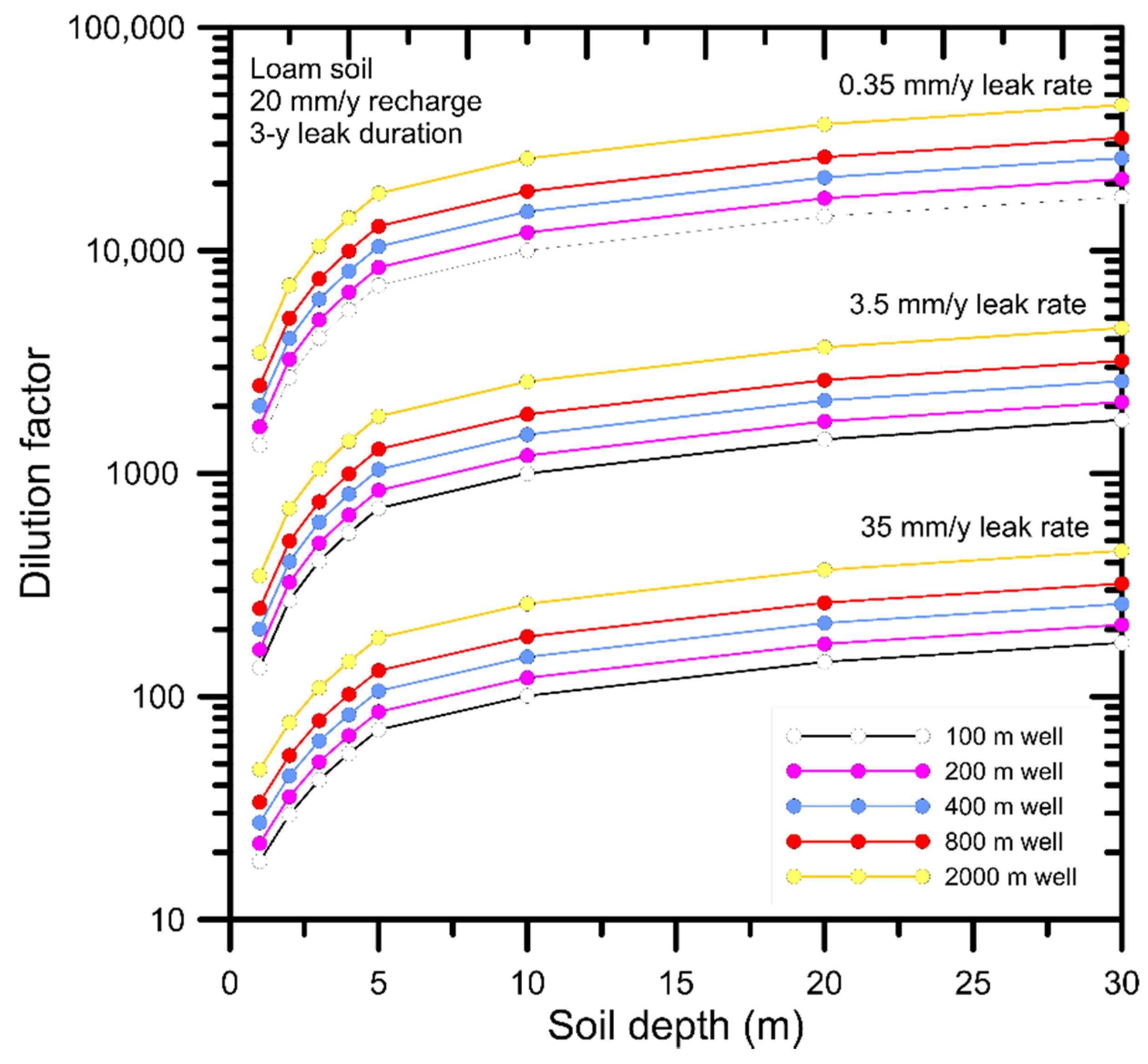
3.3. Combined Dilution Factors

The combined dilution factors (DF) from travelling through the unsaturated soil (DFL) and subsequently through groundwater (DFGW) were calculated as the product of the dilution associated with each system separately and are shown in Table 2. DF values for a three-year leak range from 1340 for the shallowest soil depth (1 m) and the 100 m water bore to just over 45,000 for the deepest soil depth (30 m) and the 2000 m water bore.
The spatial distribution of the soil depth classes shows that 66% of soils have a depth of up to 5 m, 5% between 5 to 10 m, 7% between 10 to 20 m, 4% between 20 to 30 m, and 18% have a depth larger than 30 m. These probabilities are based purely on the spatial extent of the depth to groundwater classes; there is no relationship with the occurrence of certain coal seam gas wells.

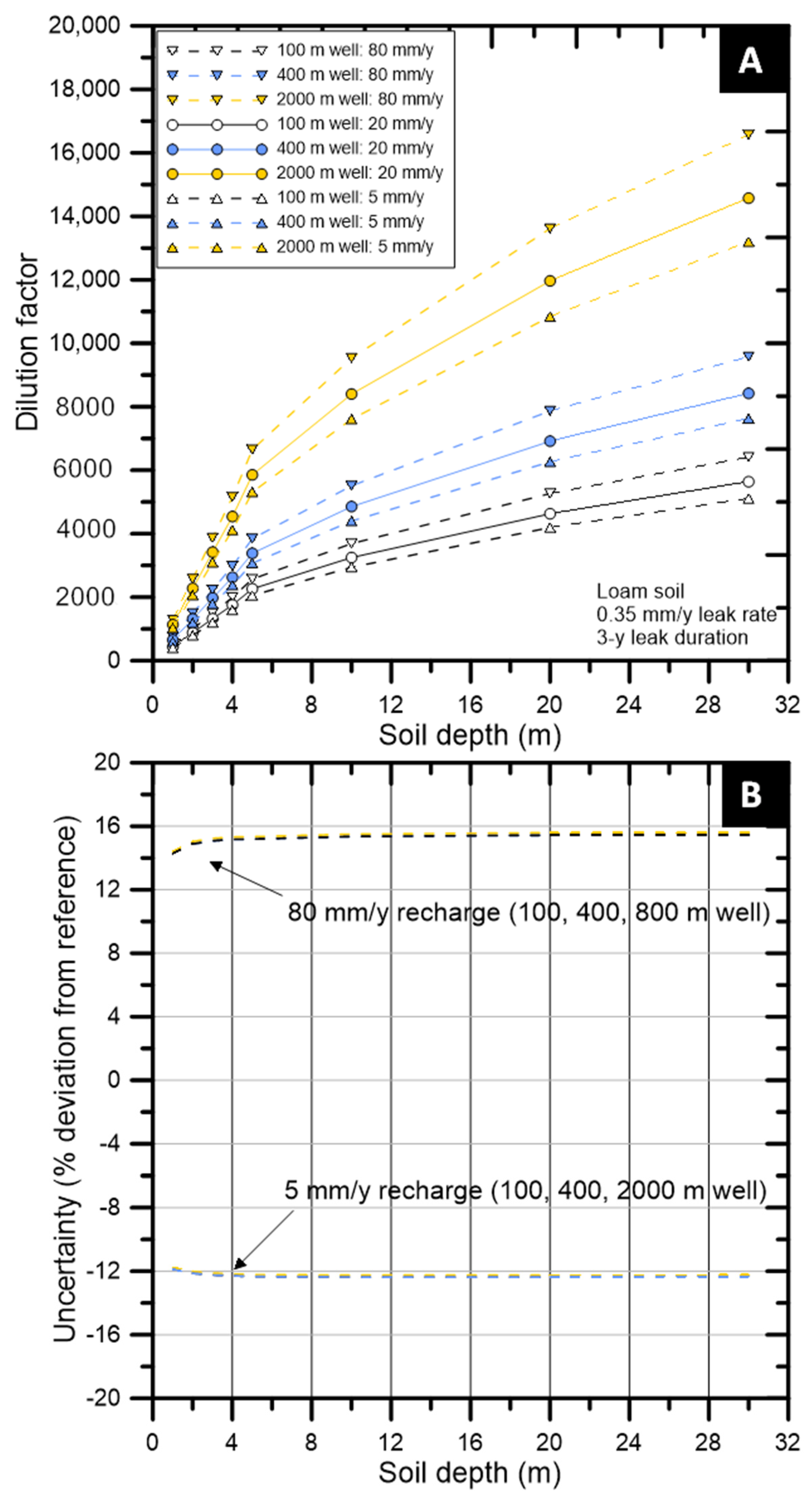
3.4. Uncertainty Propagation

The impact of the uncertainty about two key parameters—leak rate and recharge rate—on the combined soil and groundwater dilution factors were investigated next. The uncertainty around the leak rates stems mainly from uncertainty around liner performance and the long-term evolution of such performance (see Section 2.1). Uncertainty around recharge rates originates from hydroclimate variability (rainfall and evapotranspiration) combined with soil hydrologic variability (soil water balance). The propagation of uncertainty in the calculation of the dilution factor was demonstrated for different soil depths and different travel distances in groundwater. The discussion focuses first on the uncertainty in the leak rate followed by the uncertainty in the recharge rate, using loam soil as example.
The effect of the uncertainty in the leak rate (0.35–3.5–35 mm/year) produced an uncertainty in dilution factors that is more or less constant with the soil depth; for a given water bore distance, the range in dilution factors was approximately two orders of magnitude (Figure 7). The two orders of magnitude uncertainty range in input parameters (from 0.35 to 35 mm/year) returned a two orders of magnitude uncertainty in prediction (i.e., dilution factors).
Uncertainty in recharge rate is from 5 to 80 mm/year, with 20 mm/year as reference value. The propagation of uncertainty was demonstrated as function of soil depth and travel distance in groundwater for three leak rates, i.e., 0.35 mm/year (Figure 8a), and 3.5 and 35 mm/year (Figure 9). For the 0.35 mm/year leak rate, uncertainty was nearly independent of soil depth: there was a slight increase until a soil depth of 5 m, when the uncertainty (expressed as % deviation from reference, i.e., 20 mm/year) remained constant (Figure 8b). The highest recharge rate of 80 mm/year produced a slightly larger uncertainty compared to the lowest recharge of 5 mm/y, i.e., 15% (positive deviation because the 80 mm/year recharge is larger than the reference) versus 12% (negative deviation because the 5 mm/year recharge is smaller than the reference).
For the higher leak rates of 3.5 (Figure 9a) and 35 mm/year (Figure 9b) a similar behavior was observed: uncertainty (range in dilution factors) was independent of the groundwater travel distance and was nearly independent of the soil depth, except for a small increase until 5 m. Note that the magnitude of the dilution factor decreased as the leak rate increased.
The general behavior of the uncertainty propagation in dilution factors for the sand soil was very similar to that of the loam soil; the largest differences were the lower dilution factors for the sand, approximately three times less, owing to the lower water content in the sand. Propagation of uncertainty around leak rates was very similar at depths greater than 5 m; the exception was for the 35 mm/year leak rate at depths less than 5 m, for which the dilution did not increase at the same rate as it did for the lower leak rates (0.35 and 3.5 mm/year). This was due to the combined effect of a large leak rate in a relatively dry soil providing limited opportunity for dilution.

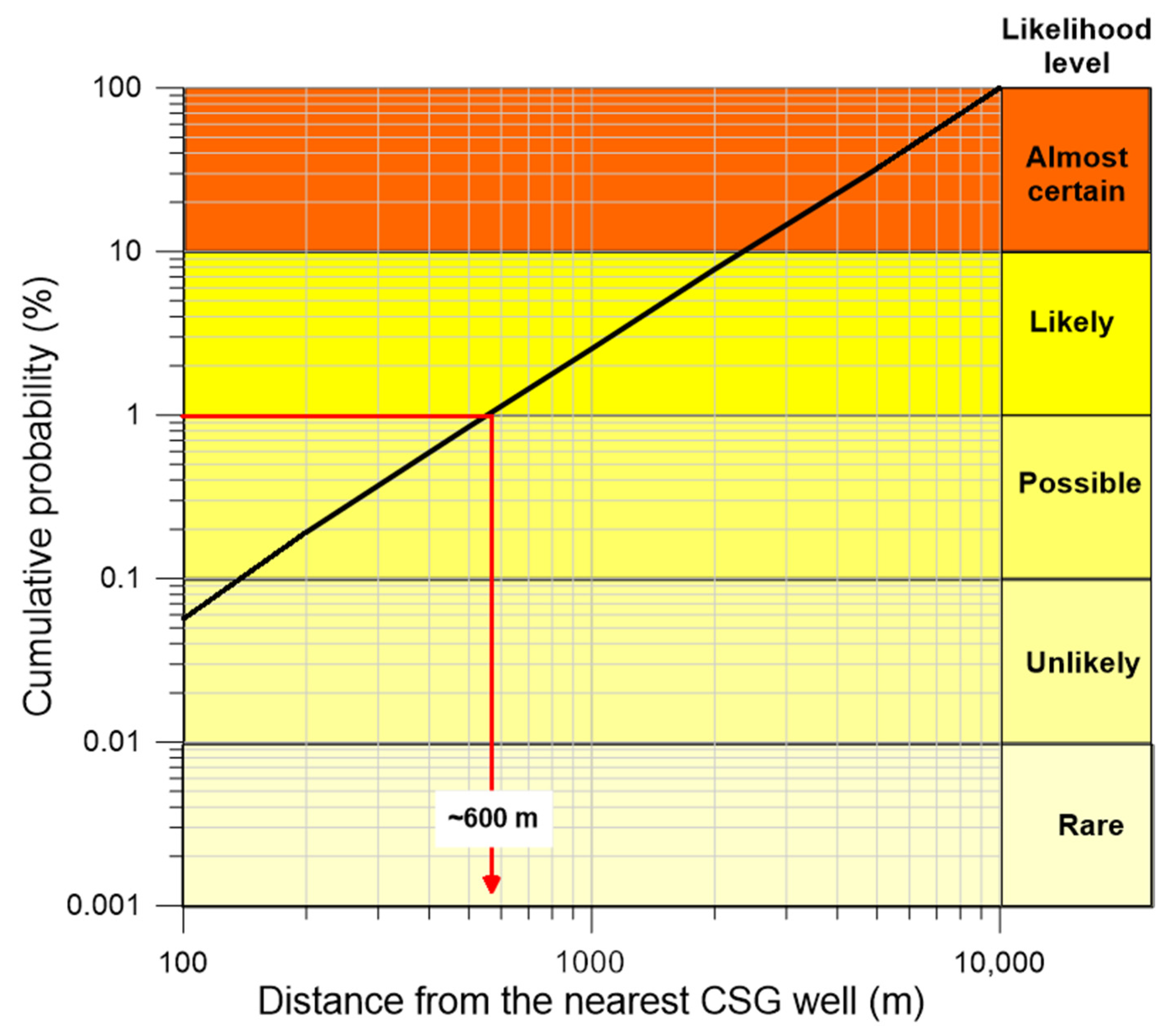
3.5. Likelihood of Dilution Factors

To assess the likelihood of occurrence for each of the different dilution factors in the case study area, the dilution factor for different travel distances and soil depth classes for the three-year leak were combined with a spatial analysis of the proximity between existing water bores and coal seam gas well using data from the Namoi catchment [80]. It was assumed for reasons of simplicity that the coordinates of the coal seam gas well corresponded to the location of a hypothetical leak (water holding pond or pipe breakage). This allowed the determination, for the currently known locations of coal seam gas wells and water bores, of the likelihood that a water bore was in close proximity to a potential contamination plume. This distance-likelihood function was then linked to the dilution factors obtained from the previous transport simulations.
The corresponding empirical cumulative distribution function of proximity between water bores and coal seam gas well is shown in Figure 10. Note that only water bores within a distance of 10,000 m were included in the graph, as at such large distances, the predicted concentrations most likely become negligible due to very large dilution factors. All water bores up to 10,000 m distance from coal seam gas wells represented 17,691 (52%) out of a total of 34,215 water bores considered in Figure 10. The cumulative distribution reveals there was only a 1% chance of finding water bores within a distance of approximately 600 m of a coal seam gas well, or, conversely, in 99% of all cases, water bores were at distances greater than approximately 600 m from a coal seam gas well. The closest distance reported between a coal seam gas and water bore was 100 m. The probability of this occurring was only 0.03% (10 out of a total of 34,215 water bores).
Similar to the likelihood analysis for proximity of water bores, the number of endangered flora species and water dependent animal species within a given radial distance from a coal seam gas well were spatially defined and quantified [60].

3.6. Predicted Environmental Concentrations for CSG Chemicals

Predicted environmental concentrations (PECs) of individual chemicals used in actual hydraulic fracturing operations were calculated for groundwater bores using Equations (5) and (6). The hydraulic fracturing chemicals were identified as being used for coal seam gas extraction in Australia between 2010 and 2012, and for which concentrations prior to injection were known [31]. From the 19 chemicals listed in Table 3, four (sodium chloride, magnesium chloride, citric acid, and guar gum) were of low concern for human health [81]. Not all of these products were used or proposed for use at any given site, and at some sites, hydraulic fracturing was neither required nor proposed [27]. The input concentrations used in Table 3 (i.e., the concentration of formulated hydraulic fracturing fluids immediately prior to injection) were based on data compiled as reported in an industry survey carried out during the Assessment [31]. The hydraulic fracturing chemicals shown in Table 3 were those for which ecotoxicological data was available for a quantitative assessment, including the derivation of predicted no-effect concentrations (PNEC) [1]. The PNEC was typically used during risk assessments to characterize the potential concern in the receiving environments.
The study of chemical mixtures and what effect this can have on organisms in the environment when they are exposed, simultaneously, to different chemicals was beyond the scope of this study. For a review of approaches to evaluate the effect of mixtures, the reader is referred to [82].
A comparison of groundwater PEC and PNEC values shows that for all but two chemicals the conservatively estimated groundwater concentration was smaller than the no-effect concentration for the protection of aquatic ecosystems. The parameters used to estimate the PECs assumed a 0.35 mm/year leak rate for a total duration of three years in a 5-m-deep loam soil under a 20 mm/year recharge rate and a groundwater bore at 100 m from the point where the solute plume enters the groundwater table. The corresponding dilution factor DF = 6980 (Table 2). The previous likelihood analysis highlighted the very low probability of 0.03% of encountering a groundwater bore within 100 m from a CSG well. In other words, for more than 99.97% of the water bores the dilution in soil and groundwater was even higher, and therefore, PNEC values were even smaller than those in Table 3. Further model assumptions that contributed to the dilution factor (and thus the PNEC) being conservative include (i) chemical interactions with the solid phase and biogeochemical transformations were ignored, (ii) continuous solute input function at the groundwater table rather than a pulse input function, causing overestimation of the maximum bore concentration by a factor of 5 at 100 m distance (for details, see [43]), and (iii) use of steady-state flow conditions that overestimate the maximum plume concentrations compared to transient flow (see, e.g., [83]).
For the two exceptions, hypochlorous acid sodium salt (or sodium hypochlorite) and guar gum, the dilution factor would need to be 360 and 1.7 larger to bring their PEC values below their respective PNEC value. The latter value of 1.7 may be obtained for a travel distance of approximately 800 m; this information can be used to set minimum separation distances between unconventional gas facilities such as water holding ponds and water bores or environmental receptors such as wetlands, streams, or sensitive ecosystems. A further increase of the DF values (by a factor 360) to reduce sodium hypochlorite concentrations below its PNEC value would require larger buffer distances and/or a control of the source concentration. We note that guar gum was identified as a polymer of low concern to human health on the basis of a set of validation rules developed to identify polymers of low concern [81].
The methodology for dilution calculations presented here is not restricted to chemicals associated with coal seam gas (or unconventional gas more broadly) activities. One of the backbones of the approach is the (uncoupled) water flow component in the vadose zone and the aquifer, both of which have broad applicability for solute migration of dissolved chemical species. Once chemical (sorption) and biological (degradation) attenuation parameters have been defined for the chemicals of interest, the current methodology can be readily applied to assess, for instance, pollution risk from soil to groundwater associated with PFAS, fertilizers and pesticides, or heavy metals.

4. Conclusions

Source-pathway-receptor modelling was undertaken for chemicals associated with coal seam gas extraction that are present in produced water temporarily stored in water holding ponds. Fluids leaking from such ponds can end up in soil and subsequently shallow groundwater; such migration results in significant solute dilution. Solute concentrations determined in soil and groundwater bores have been used to produce dilution factors for a set of leak rates and recharge rates and a broad combination of soil and groundwater parameter combinations.
Dilution factors increase with increasing recharge rate and decreasing leak rates and leak duration. Dilution in loam is roughly three times larger than in sand, irrespective of depth. This is the result of the three times higher water content in loam compared to sand. Under such conditions, chemicals entering a loam soil will be three times stronger mixed with solute-free water compared to sand.
For a hypothetical leak duration of three years, the dilution factors for the reference loam soil and reference flow conditions (0.35 mm/year leak rate and 20 mm/year recharge rate) ranged from 89 at the 1 m soil depth to 1155 at the 30 m soil depth. Increasing the 0.35 mm/year leak rate 10 or 100 times decreased the dilution factor approximately 10 or 100 times, respectively. For a 5 mm/year recharge rate the maximum dilution factor at 30 m decreased to 1013; for the 80 mm/year recharge it increased to 1334 for a 30 m deep soil profile.
Long solute transport times in the unsaturated soil provided considerable opportunity for chemical attenuation (although not calculated). In a loam soil, the earliest arrival at the groundwater table was after 152 years at 5 m depth and after 499 years at 30 m depth (leak rate of 0.35 mm/year).
Further attenuation occurred along the groundwater pathway. Dilution factors in groundwater were calculated considering typical realistic variations of key groundwater flow and solute transport parameters (aquifer hydraulic conductivity, riverbed conductance, and porosity) for wells at various distances from the chemical source. General results were that the higher the hydraulic conductivity and riverbed conductance, the greater the dilution. Dilution factors ranged from 15 for a travel distance of 100 m to 38 for a travel distance of 2000 m.
The combined soil-groundwater dilution factors across the soil-groundwater pathway were obtained by multiplying the dilution factors for soil and groundwater. Lookup tables allowed an easy determination of combined dilution by integrating the effects of parameter variations on dilution factors, and dilution from connected pathways. For a three-year leak, the combined dilution factors ranged from 1340 for the shallowest soil depth (1 m) and the 100 m water bore to just over 45,000 for the deepest soil depth (30 m) and the 2000 m water bore.
The empirical cumulative distribution function of proximity between water bores and coal seam gas wells revealed that for the most common soil depths (66% of the study area has soils from 0–5 m depth), more than 99% of the water bores had a dilution factor larger than 6980. Furthermore, for more than 99% of the water bores, the dilution in soil and groundwater was high enough to decrease the chemical concentrations of 17 out of 19 hydraulic fracturing chemicals below their PNEC values for the protection of aquatic ecosystems.
This information can be used to set minimum separation distances between unconventional gas facilities such as gas wells or water holding ponds (to avoid possible additive effects), and between gas facilities and water bores or environmental receptors such as wetlands, streams, or sensitive ecosystems. A further increase of the DF values, to reduce chemical concentrations below PNEC values, simply requires larger buffer distances and/or more stringent control of the source concentrations. In addition, the predictions could be used to strategically design a cost-effective and purpose-built monitoring network for shallow groundwater in the vicinity of surface storage ponds.
The PECs and the dilution factors obtained in this study are high-end estimates, at least for those chemicals that would normally display considerable sorption in soil. The degree of overestimation is likely several orders of magnitude, but needs confirmation through more in-depth studies including measurements of sorption behavior. Developing high-end estimates is an accepted approach when undertaking assessments with uncertain conceptual models, data, and scenarios.
Another source of uncertainty is associated with the description of the chemical source term, especially for storage ponds. More reliable data need to be collected about type of chemicals, concentration time-series, and potential leak rate from ponds. Leak monitoring data could be used to reduce such uncertainty. Furthermore, sufficient concentration of flowback and produced water has to be collected to have a broad spatial coverage of coal seam formations across Australia.

Supplementary Materials

The following are available online at https://www.mdpi.com/2073-4441/12/4/941/s1, Figure S1: Depth to water table within the alluvial groundwater modelling domains. Source: [1]. Table S1: Major soil types in the Namoi alluvium (areal coverage was derived with the ARCGISTM software). Source [1]. Table S2: Soil depth expressed as depth to groundwater based on the site groundwater flow model (24 km2). Table S3: Soil depth expressed as depth to groundwater based on the sub-regional groundwater flow model (108 km2).

Author Contributions

Conceptualization, D.M.; methodology, D.M.; software, E.B., W.S., K.M., A.T., and K.G.; formal analysis, D.M., E.B., W.S., K.M., A.T., and K.G.; writing—original draft preparation, D.M.; writing—review and editing, E.B., W.S., K.M., A.T., K.G., and B.G.; supervision, B.G.; project administration, B.G.; All authors have read and agreed to the published version of the manuscript.

Funding

This research was funded by the Office of Water Science, Department of the Environment and Energy, Australian Government.

Acknowledgments

Constructive comments from two anonymous reviewers helped improve the quality of the paper.

Conflicts of Interest

The authors declare no conflict of interest.

References

  1. DoEE. Environmental Risks Associated with Surface Handling of Chemicals Used in Coal Seam Gas Extraction, Project Report Prepared by the Chemicals and Biotechnology Assessments Section (Cbas) of the Department of the Environment and Energy (Doee) as Part of the National Assessment of Chemicals Associated with Coal Seam Gas Extraction in Australia; Commonwealth of Australia: Canberra, Australia, 2017.
  2. Balaba, R.S.; Smart, R.B. Total arsenic and selenium analysis in Marcellus shale, high-salinity water, and hydrofracture flowback wastewater. Chemosphere 2012, 89, 1437–1442. [Google Scholar] [CrossRef] [PubMed]
  3. Farag, A.M.; Harper, D.D. A review of environmental impacts of salts from produced waters on aquatic resources. Int. J. Coal Geol. 2014, 126, 157–161. [Google Scholar] [CrossRef] [Green Version]
  4. Mallants, D.; Simunek, J.; van Genuchten MTh Jacques, D. Using Hydrus and its Modules to Simulate the Fate and Transport of Coal Seam Gas Chemicals in Variably-Saturated Soils. Water 2017, 9, 385. [Google Scholar] [CrossRef] [Green Version]
  5. Skalak, K.J.; Engle, M.A.; Rowan, E.L.; Jolly, G.D.; Conko, K.M.; Benthem, A.J.; Kraemer, T.F. Surface disposal of produced waters in western and southwestern Pennsylvania: Potential for accumulation of alkali-earth elements in sediments. Int. J. Coal Geol. 2014, 126, 162–170. [Google Scholar] [CrossRef]
  6. Stearman, W.; Taulis, M.; Smith, J.; Corkeron, M. Assessment of Geogenic Contaminants in Water Co-Produced with Coal Seam Gas Extraction in Queensland, Australia: Implications for Human Health Risk. Geosciences 2014, 4, 219–239. [Google Scholar] [CrossRef] [Green Version]
  7. DiGiulio, D.C.; Jackson, R.B. Impact to Underground Sources of Drinking Water and Domestic Wells from Production Well Stimulation and Completion Practices in the Pavillion, Wyoming, Field. Environ. Sci. Technol. 2016, 50, 4524–4536. [Google Scholar] [CrossRef] [PubMed]
  8. Kahrilas, G.A.; Blotevogel, J.; Stewart, P.S.; Borch, T. Biocides in Hydraulic Fracturing Fluids: A Critical Review of Their Usage, Mobility, Degradation, and Toxicity. Environ. Sci. Technol. 2014, 49, 16–32. [Google Scholar] [CrossRef]
  9. Olsson, O.; Weichgrebe, D.; Rosenwinkel, K.H. Hydraulic fracturing wastewater in Germany: Composition, treatment, concerns. Environ. Earth Sci. 2013, 70, 3895–3906. [Google Scholar] [CrossRef]
  10. Orem, W.H.; Tatu, C.A.; Lerch, H.E.; Rice, C.A.; Bartos, T.T.; Bates, A.L.; Tewalt, S.; Corum, M.D. Organic compounds in produced waters rom coalbed natural gas wells in the Powder River Basin, Wyoming, USA. Appl. Geochem. 2007, 22, 2240–2256. [Google Scholar] [CrossRef]
  11. Rogers, J.D.; Burke, T.L.; Osborn, S.G.; Ryan, J.N. A Framework for Identifying Organic Compounds of Concern in Hydraulic Fracturing Fluids Based on Their Mobility and Persistence in Groundwater. Environ. Sci. Technol. Lett. 2015, 2, 158–164. [Google Scholar] [CrossRef] [Green Version]
  12. US EPA. Hydraulic Fracturing for Oil and Gas: Impacts from the Hydraulic Fracturing Watr Cycle on Drinking Water Resources in the United States; Office of Research and Development: Washington, DC, USA, 2016.
  13. Vengosh, A.; Jackson, R.B.; Warner, N.; Darrah, T.H.; Kondash, A. A Critical Review of the Risks to Water Resources from Unconventional Shale Gas Development and Hydraulic Fracturing in the United States. Environ. Sci. Technol. 2014, 48, 8334–8348. [Google Scholar] [CrossRef]
  14. Adgate, J.L.; Goldstein, B.D.; McKenzie, L.M. Potential public health hazards, exposures and health effects from unconventional gas development. Environ. Sci. Technol. 2014, 48, 8307–8320. [Google Scholar] [CrossRef]
  15. Groat, C.G.; Grimshaw, T.W. Fact-Based Regulation for Environmental Protection in Shale Gas Development; The Energy Institute, University of Texas at Austin: Austin, TX, USA, 2012. [Google Scholar]
  16. Flewelling, S.A.; Sharma, M. Constraints on Upward Migration of Hydraulic Fracturing Fluid and Brine. Groundwater 2014, 52, 9–19. [Google Scholar] [CrossRef] [PubMed] [Green Version]
  17. Jeffrey, R.; Wu, B.; Bunger, A.; Zhang, X.; Chen, Z.; Kear, J.; Kasperczyk, D. Literature Review: Hydraulic Fracture Growth and Well Integrity, Project Report Prepared by the Commonwealth Scientific and Industrial Research Organisation (CSIRO) as Part of the National Assessment of Chemicals Associated with Coal Seam Gas Extraction in Australia; Commonwealth of Australia: Canberra, Australia, 2017.
  18. Mallants, D.; Bekele, E.; Schmid, W.; Miotlinski, K.; Bristow, K. Literature Review: Identification of Potential Pahways to Shallow Groundwater of Fluids Associated with Hydraulic Fracturing, Project Report Prepared by the Commonwealth Scientific and Industrial Research Organisation (CSIRO) as Part of the National Assessment of Chemicals Associated with Coal Seam Gas Extraction in Australia; Commonwealth of Australia: Canberra, Australia, 2017.
  19. Myers, T. Potential contaminant pathways from hydraulically fractured shale to aquifers. Groundwater 2012, 50, 872–882. [Google Scholar] [CrossRef] [PubMed]
  20. Rozell, D.J.; Reaven, S.J. Water pollution risk associated with natural gas extraction from the Marcellus Shale. Risk Anal. 2012, 32, 1382–1393. [Google Scholar] [CrossRef] [PubMed]
  21. Rutovitz, J.; Harris, S.M.; Kuruppu, N.; Dunstan, C. Drilling down: Coal Seam Gas-a Background Paper, Institute for Sustainable Futures; University of Technology Sydney (UTS): Sydney, Australia, 2011; pp. 1–83. Available online: http://cfsites1.uts.edu.au/find/isf/publications/rutovitzetal2011sydneycoalseamgasbkgd.pdf (accessed on 12 October 2015).
  22. Stringfellow, W.T.; Domen, J.K.; Camarillo, M.K.; Sandelin, W.L.; Borglin, S. Physical, chemical, and biological characteristics of compounds used in hydraulic fracturing. J. Hazard. Mater. 2014, 275, 37–54. [Google Scholar] [CrossRef] [PubMed]
  23. The Royal Society and Royal Academy of Engineering. Shale Gas Extraction in the UK: A Review of Hydraulic Fracturing; The Royal Society and Royal Academy of Engineering: London, UK, 2012. [Google Scholar]
  24. Vidic, R.D.; Brantley, S.L.; Vandenbossche, J.M.; Yoxtheimer, D.; Abad, J.D. Impact of shale gas development on regional water quality. Science 2013, 340, 6134. [Google Scholar] [CrossRef] [PubMed] [Green Version]
  25. Dusseault, M.; Jackson, R. Seepage pathways assessment for natural gas to shallow groundwater during well stimulation, in production, and after abandonment. Environ. Geosci. 2014, 21, 107–126. [Google Scholar] [CrossRef]
  26. Engelder, T.; Cathless, L.M.; Bryndzia, L.T. The fate of residual treatment water in gas shale. J. Unconv. Oil Gas Resour. 2014, 7, 33–48. [Google Scholar] [CrossRef]
  27. Mallants, D.; Jeffrey, R.; Kear, J.; Chen, Z.; Wu, B.; Bekele, E.; Apte, S.; Gray, B. Review of migration pathways for hydraulic fracturing chemicals. Int. J. Coal Geol. 2018, 195, 280–303. [Google Scholar] [CrossRef]
  28. Lechtenböhmer, S.; Altmann, M.; Capito, S.; Matra, Z.; Weindorf, W.; Zittel, W. Impacts of Shale Gas and Shale Oil Extraction on the Environment and on Human Health, Wuppertal Institute for Climate, Environment and Energy and Ludwig-Bölkow-Systemtechnik GmbH, Study Requested by the European Parliament’s Committee on Environment; Public Health and Food Safety: Brussels, Belgium, 2011. [Google Scholar]
  29. Mastrandrea, M.D.; Field, C.B.; Stocker, T.F.; Edenhofer, O.; Ebi, K.L.; Frame, D.J.; Held, H.; Kriegler, E.; Mach, K.J.; Matschoss, P.R.; et al. Guidance Note for Lead Authors of the IPCC Fifth Assessment Report on Consistent Treatment of Uncertainties; Intergovernmental Panel on Climate Change (IPCC): Geneva, Switzerland, 2011. [Google Scholar]
  30. DERM. CSG/LNG Compliance Plan 2011 Update: January 2011 to June 2011; Department of Environment and Resource Management: Brisbane, Australia, 2011. Available online: http://www.ehp.qld.gov.au/management/coal-seam-gas/pdf/csg-lng-compliance-update1.pdf (accessed on 12 October 2015).
  31. NICNAS. Identification of Chemicals Associated with Coal Seam Gas Extraction in Australia, Project Report Prepared by the National Industrial Chemicals Notification and Assessment Scheme (NICNAS) as Part of the National Assessment of Chemicals Associated with Coal Seam Gas Extraction in Australia; Commonwealth of Australia: Canberra, Australia, 2017.
  32. NICNAS. Human Health and Environmental Risks Associated with Surface Spills and Leaks of Chemicals, Project Report, Report Prepared by the National Industrial Chemicals Notification and Assessment Scheme (NICNAS) as Part of the National Assessment of Chemicals Associated with Coal Seam Gas Extraction in Australia; Commonwealth of Australia: Canberra, Australia, 2017.
  33. Chapuis, R.P. Full-scale hydraulic performance of soil–bentonite and compacted clay liners. Can. Geotech. J. 2002, 39, 417–439. [Google Scholar] [CrossRef]
  34. Council of Canadian Academies. Environmental Impacts of Shale Gas Extraction in Canada; Council of Canadian Academies: Ottawa, ON, Canada, 2014. [Google Scholar]
  35. Giroud, J.P.; Bonaparte, R. Leakage through liners constructed with geomembranes -1. Geomembrane liners. Geotext. Geomembr. 1989, 8, 27–67. [Google Scholar] [CrossRef]
  36. Rowe, R.K. Short- and long-term leakage through composite liners, the 7th Arthur Casagrande Lecture. Can. Geotech. J. 2012, 49, 141–169. [Google Scholar] [CrossRef] [Green Version]
  37. Benson, C.H. Waste containment: Strategies and Performance. Aust. Geomech. 2001, 36, 1–25. [Google Scholar]
  38. Folkes, D.J. Control of contaminant migration by the use of liners. Can. Geotech. J. 1982, 19, 320–344. [Google Scholar] [CrossRef]
  39. Rowe, R.K.; Quigley, R.M.; Brachman, R.W.I.; Booker, J.R. Barrier Systems for Waste Disposal Facilities; Taylor and Francis Books Ltd. (E and FN Spon): London, UK, 2004. [Google Scholar]
  40. Rowe, R.K.; Hosney, M.S. A systems engineering approach to minimizing leachate leakage from landfills. In Proceedings of the 9th International Conference on Geosynthetics, Guaruja, Brazil, 23–27 May 2010; pp. 501–510. [Google Scholar]
  41. Bonaparte, R.; Daniel, D.; Koerner, R.M. Assessment and Recommendations for Improving the Performance of Waste Containment Systems; EPA Report EPA/600/R-02/099; U.S. Environmental Protection Agency (US EPA): Washington, DC, USA, 2002.
  42. Beck, A.L. A Statistical Approach to Minimizing Landfill Leakage. In Proceedings of the Solid Waste Association of North America (SWANA) Wastecon, Washington, DC, USA, 14–16 August 2012. [Google Scholar]
  43. Mallants, D.; Bekele, E.; Schmid, W.; Miotlinski, K.; Taylor, A.; Gerke, K. Human and Environmental Exposure Assessment: Soil to Shallow Groundwater Pathways—A Study of Predicted Environmental Concentrations, Project Report Prepared by the Commonwealth Scientific and Industrial Research Organisation (CSIRO) as Part of the National Assessment of Chemicals Associated with Coal Seam Gas Extraction in Australia; Commonwealth of Australia: Canberra, Australia, 2017.
  44. Mallants, D.; Apte, S.; Kear, J.; Turnadge, C.; Janardhanan, S.; Gonzalez, D.; Williams, M.; Chen, Z.; Kookana, R.; Taylor, A.; et al. Deeper Groundwater Hazard Screening Research; The Commonwealth Scientific and Industrial Research Organisation (CSIRO): Canberra, Australia, 2017. [Google Scholar]
  45. USEPA. Soil Screening Guidance: Technical Background Document; EPA/540/R95/12.8; Office of Solid Waste and Emergency Response, US Environmental Protection Agency: Washington, DC, USA, 1996.
  46. Van Genuchten, M.T.H. A closed-form equation for predicting the hydraulic conductivity of unsaturated soils. Soil Sci. Soc. Am. J. 1980, 44, 892–898. [Google Scholar] [CrossRef] [Green Version]
  47. Mualem, Y. A new model for predicting the hydraulic conductivity of unsaturated porous media. Water Resour. Res. 1976, 12, 513–522. [Google Scholar] [CrossRef] [Green Version]
  48. Mallants, D.; van Genuchten MTh Simunek, J.; Jacques, D.; Seetharam, S. Leaching of contaminants to groundwater—Chapter 18. In Dealing with Contaminated Sites. from Theory towards Practical Application; Swartjens, F., Ed.; Springer: Dordrecht, The Netherlands, 2011; pp. 787–850. ISBN 978-90-481-9756-9. [Google Scholar] [CrossRef]
  49. Šimůnek, J.; Sejna, M.; Saito, H.; Sakai, M.; van Genuchten, M.T. The HYDRUS-1D Software Package for Simulating the Movement of Water, Heat, and Multiple Solutes in Variably Saturated Media, Version 4.08; HYDRUS Software Series 3; Department of Environmental Sciences, University of California Riverside: Riverside, CA, USA, 2009; p. 330. [Google Scholar]
  50. Rassam, D.; Šimůnek, J.; Mallants, D.; van Genuchten, M.T. The HYDRUS-1D Software Package for Simulating the Movement of Water, Heat, and Multiple Solutes in Variably Saturated Media: Tutorial, Version 1.00; CSIRO Land and Water: Canberra, Australia, 2018; p. 183. ISBN 978-1-4863-1001-2. [Google Scholar]
  51. Gerke, K.M.; Sidle, R.C.; Mallants, D. Preferential flow mechanisms identified from staining experiments in forested hillslopes. Hydrol. Process. 2015, 29, 4562–4578. [Google Scholar] [CrossRef]
  52. Vanderborght, J.; Vereecken, H. Review of dispersivities for solute transport modeling in soils. Vadose Zone J. 2007, 6, 29–52. [Google Scholar] [CrossRef]
  53. US EPA. Overview of the Ecological Risk Assessment Process in the Office of Pesticide Programs; Report Prepared by the Office of Prevention, Pesticides and Toxic Substances and Office of Pesticide Programs for the US Environmental Protection Agency (USEPA); US EPA: Washington, DC, USA, 2004.
  54. McNeilage, C. Upper Namoi Groundwater Flow Model, Model Development and Calibration; NSW Government Department of Natural Resources: Parramatta, Australia, 2006.
  55. Sun, H.; Cornish, P.S. A catchment-based approach to recharge estimation in the Liverpool Plains, NSW Australia. Aust. J. Agric. Res. 2006, 57, 309–320. Available online: http://www.publish.csiro.au/cp/AR04015 (accessed on 12 October 2015). [CrossRef]
  56. Zhang, L.; Stauffacher, M.; Walker, G.R.; Dyce, P. Recharge Estimation in the Liverpool Plains (Nsw) for Input to Groundwater Models; CSIRO Land and Water Technical Report 10/97; CSIRO: Canberra, Australia, 1997.
  57. Daniells, I.G.; Brown, R.; Deegan, L. (Eds.) Northern Wheat-belt SOILpak. NSW Agriculture: Tamworth, UK, 1994; p. 47. [Google Scholar]
  58. Carsel, R.F.; Parrish, R.S. Developing joint probability distributions of soil water retention characteristics. Water Resour. Res. 1988, 24, 755–769. [Google Scholar] [CrossRef] [Green Version]
  59. Soil Survey Staff. Keys to Soil Taxonomy. United States Department of Agriculture-Natural Resources Conservation Service, 12th ed.; NRCS: Lincoln, NE, USA, 2014.
  60. Mallants, D.; Bekele, E.; Schmid, W.; Miotliński, K. Human and Environmental Exposure Conceptualisation: Soil to Shallow Groundwater Pathways, Project Report Prepared by the Commonwealth Scientific and Industrial Research Organisation (CSIRO) as Part of the National Assessment of Chemicals Associated with Coal Seam Gas Extraction in Australia; Commonwealth of Australia: Canberra, Australia, 2017.
  61. SWS. The Namoi Catchment Water Study Independent Expert Final Study Report, Prepared by Schlumberger Water Services for the Department of Trade and Investment; Regional Infrastructure and Services, NSW (DTIRIS NSW): Sydney, Australia, 2012.
  62. SWS. Namoi Catchment Water Study Independent Expert Phase 3 Report, Prepared by Schlumberger Water Services for the Department of Trade and Investment; Regional Infrastructure and Services, NSW (DTIRIS NSW): Sydney, Australia, 2012.
  63. Engesgaard, P.; Jensen, K.H.; Molson, J.; Frind, E.O.; Olsen, H. Large-scale dispersion in a sandy aquifer: Simulation of subsurface transport of environmental tritium. Water Resour. Res. 1996, 32, 3253–3266. [Google Scholar] [CrossRef]
  64. Mallants, D.; Espino, A.; Van Hoorick, M.; Ferson, S.; Feyen, J.; Vandenberghe, N.; Loy, W. Dispersivity estimates from a tracer test in a sandy aquifer. Groundwater 2000, 38, 304–310. [Google Scholar] [CrossRef]
  65. Sudicky, E.A.; Illman, W.A.; Goltz, I.K.; Adams, J.J.; McLaren, R.G. Heterogeneity in hydraulic conductivity and its role on the macroscale transport of a solute plume: From measurements to a practical application of stochastic flow and transport theory. Water Resour. Res. 2010, 46, W01508. [Google Scholar] [CrossRef]
  66. Gedeon, M.; Mallants, D. Description of the hydrogeology. In Project Near Surface Disposal of Category a Waste at Dessel; NIRAS/ONDRAF: Brussel, Belgium, 2009; p. 174. [Google Scholar]
  67. Mehl, S.; Hill, M.C. MODFLOW-2005, the U.S. geological survey modular ground-water model. In Documentation of Local Grid Refinement (LGR) and the Boundary Flow and Head (BFH) Package; US Geological Survey Techniques and Methods 6-A12; US Geological Survey: Denver, CO, USA, 2005; p. 68. [Google Scholar]
  68. Zheng, C.; Wang, P. MT3DMS: A Modular Three-Dimensional Multispecies Transport Model for Simulation of Advection, Dispersion, and Chemical Reactions of Contaminants in Groundwater Systems; Documentation and User’s Guide; US Army Corps of Engineers: Washington, DC, USA, 1999.
  69. Gelhar, L.W.; Welty, C.; Rehfeldt, K.R. A critical overview of data on field-scale dispersion in aquifers. Water Resour. Res. 1992, 28, 1955–1974. [Google Scholar] [CrossRef]
  70. Anderson, M.P.; Cherry, J.A. Using models to simulate the movement of contaminants through groundwater flow systems. Crit. Rev. Environ. Sci. Technol. 1979, 9, 97–156. [Google Scholar] [CrossRef]
  71. Rumbaugh, J.; Rumbaugh, D. Groundwater Vistas, Tutorial Manual for Groundwater Vistas; Version 6; Environmental Simulations; Reinholds: Lancaster County, PA, USA, 2011. [Google Scholar]
  72. Barnett, B.; Townley, L.R.; Post, V.; Evans, R.E.; Hunt, R.J.; Peeters, L.; Richardson, S.; Werner, A.D.; Knapton ABoronkay, A. Australian Groundwater Modelling Guidelines; Waterlines Report Series No 82, June 2012; Sinclair Knight Merz and the National Centre for Groundwater Research and Training for the National Water Commission: Canberra, Australia, 2012. [Google Scholar]
  73. Flury, M.; Fluhler, H.; Jury, W.; Leuenberger, J. Susceptibility of soils to preferential flow of water: A field study. Water Resour. Res. 1994, 30, 1945–1954. [Google Scholar] [CrossRef]
  74. Hendrickx, J.M.H.; Flury, M. Uniform and preferential flow, mechanisms in the Vadose zone. In Conceptual Models of Flow and Transport in the Fractured Vadose Zone; National Research Council, National Academy: Washington, DC, USA, 2001; pp. 149–187. [Google Scholar]
  75. Mallants, D. Field-scale solute transport parameters derived from tracer tests in large undisturbed soil columns. Soil Res. 2014, 52, 13–26. [Google Scholar] [CrossRef]
  76. Šimůnek, J.; van Genuchten, M.T.H. Contaminant transport in the unsaturated zone: Theory and modeling, chapter 22. In The Handbook of Groundwater Engineering, 2nd ed.; Delleur, J., Ed.; CRC: Boca Raton, FL, USA, 2006; pp. 22.1–22.46. [Google Scholar]
  77. Palmer, C.D.; Johnson, R.L. Physical Processes Controlling the Transport of Contaminants in the Aqueous Phase: Transport and Fate of Contaminants in the Subsurface; U.S. Environmental Protection Agency, Center for Environmental Research Information: Cincinnati, OH, USA; Robert S. Kerr Environmental Research Laboratory: Ada, OK, USA, 1989.
  78. USEPA. Guidelines for Exposure Assessment; Federal Register 57:22888-22938. EPA/600/Z-92/001 May 1992; U.S. Environmental Protection Agency: Washington, DC, USA, 1992; p. 139. Available online: http://cfpub.epa.gov/ncea/cfm/recordisplay.cfm?deid=15263#Download (accessed on 12 October 2015).
  79. USEPA. Determination of Groundwater Dilution Attenuation Factors for Fixed Waste Site Areas Using EPACMTP-Appendix E; US Environmental Protection Agency Office of Solid Waste: Washington, DC, USA, 1994.
  80. NSW Government. Pinneena Database, New South Wales Government. 2014. Available online: waterinfo.nsw.gov.au/pinneena/ (accessed on 12 October 2015).
  81. NICNAS. Chemicals of Low Concern for Human Health, Project Report Prepared by the National Industrial Chemicals Notification and Assessment Scheme (NICNAS) as Part of the National Assessment of Chemicals Associated with Coal Seam Gas Extraction in Australia; Commonwealth of Australia: Canberra, Australia, 2017.
  82. Heys, K.A.; Shore, R.F.; Pereira, M.G.; Jones, K.C.; Martin, F.L. Risk assessment of environmental mixture effects. RSC Adv. 2016, 6, 47844–47857. [Google Scholar] [CrossRef] [Green Version]
  83. Gedeon, M.; Mallants, D. Sensitivity analysis of a combined groundwater flow and solute transport model using local-grid refinement: A case study. Math. Geosci. 2012, 44, 881–900. [Google Scholar] [CrossRef]
Figure 1. Possible contaminant sources at the coal seam gas site (1 to 5), migration pathways in shallow (10) and deep (6 to 8) groundwater, and via surface runoff (9) during the depressurization phase. Source: [27].
Water 12 00941 g001
Figure 2. Plan view (A) and cross section view (B) of components of the soil-groundwater pathway used to assess solute migration from storage ponds via soil and groundwater pathways. Each component provides a set of computational endpoints. For derivation of dilution factors for unsaturated and saturated zone, see the main text [45].
Water 12 00941 g002
Figure 3. Example of hydraulic conductivity curves (A) and soil water retention curves (B) for the sand, loam, and clay soil textural classes. Source: based on soil hydraulic parameters from [58].
Water 12 00941 g003
Figure 4. Developing a detailed small-scale site groundwater model (grid cells are 50 × 50 m2 each) for solute transport simulation within a local (sub-regional) groundwater model (108 km2 with grid cells of 1 × 1 km2 each) using the local grid refinement (LGR) method.
Water 12 00941 g004
Figure 5. Example solute plume after 1500 years following a long-term release from a leaking storage pond. A unit input concentration at the soil–groundwater interface is assumed (i.e., C0 = 1 mg/L). Solute concentrations are collected at 100, 200, 400, 800, and 2000 m.
Water 12 00941 g005
Figure 6. Soil dilution factor (DFL) as function of soil depth for loam soil. DFL is calculated at the soil-groundwater interface (three-year leak).
Water 12 00941 g006
Figure 7. Combined dilution factor (DF) for loam soil and groundwater. Reference groundwater conditions used.
Water 12 00941 g007
Figure 8. Combined dilution factor (DF) for loam soil (0.35 mm/year leak rate) with three recharge rates and groundwater pathway for reference groundwater conditions (A). Uncertainty (in % deviation from reference) as function of soil depth, groundwater travel distance, and recharge rate (B).
Water 12 00941 g008
Figure 9. Combined dilution factor (DF) for loam soil and groundwater pathway. Reference groundwater conditions used. Loam soil with three recharge rates and leak rates of 3.5 mm/year (A) and 35 mm/year (B).
Water 12 00941 g009
Figure 10. Empirical cumulative distribution of proximity between water bores and coal seam gas wells for the Narrabri catchment.
Water 12 00941 g010
Table 1. Dilution factors in groundwater for different values of aquifer hydraulic conductivity (K) and riverbed conductance. Gradient was modified by changing riverbed conductance: L = low, M = medium, H = high. Dilution factors are identical for different porosities (0.1, 0.2, and 0.4). Results have been rounded to two significant numbers. nc = not calculated because solute plume bypasses the water bore at 2000 m.
Distance to Water BoreHydraulic Conductivity, K
Low KReference KHigh K
Riverbed ConductanceRiverbed ConductanceRiverbed Conductance
LMHLMHLMH
100 m3.02.99.6151520596066
200 m3.83.515181824707077
400 m4.94.437242331848593
800 m6.46.5469322857103104120
2000 m1527Nc5738nc142142212
Table 2. Combined dilution factor for the soil-groundwater pathway for the loam soil and groundwater reference cases (three-year leak period, 0.35 mm/year leak rate, 20 mm/year recharge).
Bore Distance→100 m200 m400 m800 m2000 m
Soil Depth↓
1 m13401613199924663450
2 m27003246402549656968
3 m405048766055746510,478
4 m541065168085996513,988
5 m6980839610,42512,85518,038
10 m999512,03814,93218,41825,839
20 m14,24517,13821,27226,23836,799
30 m17,43520,99126,04332,11945,055
Table 3. Calculated groundwater predicted environmental concentrations (PECs) for chemicals present in hydraulic fracturing products or fracturing pre-treatment formulations (loam soil parameters: 0.35 mm/year leak rate, 5 m soil depth, 20 mm/year recharge, three-year leak duration; reference groundwater parameters, water bore at 100 m). Source: concentration after final dilution based on [32]; Predicted no-effect concentration (PNEC) for the protection of aquatic freshwater biota based on [1]. @Revised water quality guideline submitted to the Department of Agriculture and Water Resources, September 2016 (very high reliability). #chemical of low concern for human health.
CAS No.CAS Chemical Name (Common Name/Formula)Concentration after Final Dilution Prior to Injection (g/kg or g/L)Groundwater PEC (mg/L)PNEC (mg/L)
10,043-35-3Boric acid (H3BO3)0.2160.0310.83@
107-21-11,2-Ethanediol (Ethylene glycol)0.4960.07110
111-76-22-Butoxyethanol (Butoxyethanol)0.040.00570.165
1310-73-2Sodium hydroxide (Na(OH))0.13750.0202.4
26,172-55-43(2H)-Isothiazolone, 5-chloro-2-methyl- (Methyl-chloroisothiazolinone)0.00370.000530.00062
2682-20-43(2H)-Isothiazolone, 2-methyl- (Methyliso-thiazolone)0.00110.000160.0007
497-19-8Carbonic acid sodium salt (1:2) (Soda ash)0.3160.0454.24
55,566-30-8Phosphonium, tetrakis(hydroxymethyl)-, sulfate (2:1) (salt) (THPS)0.041250.00590.94
64-19-7Acetic acid (Acetic acid)0.5250.07515
67-63-02-Propanol (Isopropanol)0.01340.0019500
7447-40-7Potassium chloride (KCl)22.963.33.73
75-57-0Methanaminium, N,N,N-trimethyl-, chloride (1:1) (Tetramethylammonium chloride)1.2730.184.62
7647-14-5#Sodium chloride (Common salt)0.40.0573.14
7647-01-0Hydrochloric acid (Hydrochloric acid)0.05250.00756.2
7681-52-9Hypochlorous acid, sodium salt (1:1) (Sodium hypochlorite)0.05780.00830.000023
7727-54-0Peroxydisulfuric acid ([(HO)S(O)2]2O2), ammonium salt (1:2) (Ammonium persulfate)0.45210.0650.92
7786-30-3#Magnesium chloride (MgCl2)0.00340.000492.12
77-92-9#1,2,3-Propanetricarboxylic acid, 2-hydroxy- (citric acid)1.7650.2515.3
9000-30-0#Guar gum (Guar gum)2.60.370.22

