Modified Maximum Pseudo Likelihood Method of Copula Parameter Estimation for Skewed Hydrometeorological Data

Abstract

For multivariate frequency analysis of hydrometeorological data, the copula model is commonly used to construct joint probability distribution due to its flexibility and simplicity. The Maximum Pseudo-Likelihood (MPL) method is one of the most widely used methods for fitting a copula model. The MPL method was derived from the Weibull plotting position formula assuming a uniform distribution. Because extreme hydrometeorological data are often positively skewed, capacity of the MPL method may not be fully utilized. This study proposes the modified MPL (MMPL) method to improve the MPL method by taking into consideration the skewness of the data. In the MMPL method, the Weibull plotting position formula in the original MPL method is replaced with the formulas which can consider the skewness of the data. The Monte-Carlo simulation has been performed under various conditions in order to assess the performance of the proposed method with the Gumbel copula model. The proposed MMPL method provides more precise parameter estimates than does the MPL method for positively skewed hydrometeorological data based on the simulation results. The MMPL method would be a better alternative for fitting the copula model to the skewed data sets. Additionally, applications of the MMPL methods were performed on the two weather stations (Seosan and Yeongwol) in South Korea.

1. Introduction

Hydrological phenomena have multidimensional characteristics; therefore, more than one variable is required to be considered in simultaneous analyses of the hydrological phenomena [1]. The multivariate probability model accounts for the multidimensional characteristics. However, traditional multivariate probability models that are widely used in the analysis of hydrological data were derived on the basis of univariate probability distribution [2,3,4,5,6]. They assume that random variables follow the distribution model that is utilized in the derivation of multivariate probability distribution model [7]. Hence, they provide limited performances for analysis of the random variables when each random variable follows a different distribution model.

The copula model has been widely adopted as an alternative to mitigate the limitation of the traditional multivariate probability model in the frequency analysis of multidimensional data. In field of the hydrology, the copula model has been used in the analyses of various hydrometeorological phenomena, such as rainfall, flood, drought, and groundwater. For modeling rainfall events, a rainfall event can be characterized by rainfall volume, duration, and intensity. Reference [8] performed a bivariate frequency analysis of extreme rainfall events to determine design criteria of hydro-infrastructure. Two of the total volume, duration, and peak intensity were selected as random variables of the bivariate probability distribution. Reference [9] investigated bivariate frequency analysis of rainfall data specifically for urban infrastructure design. They employed the copula model to derive more realistic design storms.

For drought, many studies have modeled and analyzed drought characteristics and indices, such as SPI, SPEI, and PDSI [10,11,12,13,14]. Since droughts are characterized by more than one variable, the copula model has gained popularity in risk assessment of drought [15]. Reference [16] analyzed droughts by utilizing three variables (duration, severity, and minimum flow) with bivariate and trivariate Plakett copulas. Reference [17] showed multi-site real-time assessment of droughts with variables of drought duration and average intensity. Reference [18] developed a regional drought frequency analysis based on trivariate copulas by considering the spatio-temporal variations of drought events.

Flood characteristics can be characterized by peak discharge, flood volume, and duration. Reference [19] derived bivariate distributions of flood peak and volume, as well as flood volume and duration, by using the copula model for flood data of Louisiana and Canada. Reference [20] performed flood frequency analysis and compared return periods of univariate and multivariate probability distributions.

Since use of the copula model has been widely used for hydrometeorological data, accurate estimation of copula parameter has become an important issue to be investigated. Reference [21] suggested the semiparametric estimator based on dependence measurement, such as Kendall’s tau (τ) statistic for Archimedean copula, which is called method of moments (by using the function relationship between copula parameter and dependence measure) or Non-Parametric (NP) method. But the NP method cannot be applicable for all of the copulas when a direct relation between the copula parameter and Kendall’s tau does not exist [10].

Reference [22] proposed the copula parameter estimator by using a pseudo-likelihood which is called the Maximum Pseudo-Likelihood (MPL) method or canonical maximum likelihood method. In this method, before estimating the copula parameter, the marginal empirical distribution function is converted by $R/\left(n+1\right)$, where $R$ is rank of the data and $n$ is the sample size. This Weibull plotting position formula could underestimate the return period due to its own formula as referred by Reference [23]. As a parametric inference, Reference [24] suggested the estimation method of Inference Functions for Margins (IFM) for multivariate models. This method makes inference computationally feasible for many multivariate models. Other notable methods have also been recently developed. Reference [25,26] performed bivariate frequency analysis under the Bayesian paradigm for flood and drought, respectively. Furthermore, Reference [27] developed the Multivariate Copula Analysis Toolbox (MvCAT) which includes 26 copula families and a Bayesian parameter estimation framework. Reference [28] introduced a new estimation method for bivariate copula parameters with bivariate L-moments and performed extensive simulation experiment.

Among these parameter estimation methods, the MPL method is one of the most popular methods due to its simplicity and flexibility. However, skewness of the random variable may degrade the capacity of the MPL method because of the Weibull plotting position formula. Since most hydrometeorological data in extreme frequency analysis have a positive coefficient of skewness, the MPL method should be modified to improve the accuracy of parameter estimation.

This study proposes the modified maximum pseudo-likelihood (MMPL) method by replacing the plotting position formula, which considers skewness of the data in the bivariate case. Various plotting position formulas were tested for the MMPL method. To evaluate the performance of the MMPL method for copula, a simulation experiment was carried out with various conditions, such as dependence between variables, marginal distribution type, sample size, and coefficient of skewness. Its performance was compared to the performance of the MPL and IFM methods for conventional semi-parametric and parametric methods. A bivariate frequency analysis of extreme rainfall events in South Korea was then performed for a case study of a real data set. Performances of the three tested methods were evaluated in the case study. Results of this study may provide an alternative to fit the copula model in multivariate frequency analysis of the hydrometeorological variables.

This study is organized as follows: Section 2 describes theoretical backgrounds about copula and conventional parameter estimation methods. Section 3 describes the MMPL method. Section 4 presents the simulation procedure and its results. Section 5 includes application contents for weather stations in South Korea. Section 6 includes a discussion on the results of this paper, and Section 7 presents the conclusions.

2. Theoretical Background

2.1. Copula Model

The copula model was first suggested by Reference [29]. A copula function is a joint multivariate distribution that binds each univariate distribution on [0,1]. The $d$-dimensional copula function can be expressed simply as $C:{\left[0,1\right]}^d\to \left[0,1\right]$ and is defined in Equation (1):

$$H\left[x_1,x_2,\dots ,x_d\right]=C\left[F_1\left(x_1\right),F_2\left(x_2\right),\dots ,F_d\left(x_d\right)\right]=C\left(u_1, u_2, \dots , u_d\right)$$

(1)

where $H$ is the joint probability, $C$ is the copula function, $x_i$ is a random variable, $F_i$ is the marginal distribution of the $i$-th random variable that can be considered as the cumulative distribution function (CDF) of $i$-th random variable, and $u_i$ is a non-exceedance probability of marginal distribution variable of the copula function.

Archimedean copulas have been broadly and frequently used for modeling hydrometeorological data because it is easy to derive their probability functions and estimate their parameters [12,30,31,32,33,34]. A bivariate Archimedean copula $C$ is a solution of the functional equation

$$C\left(u, v\right)={\phi }^{-1}\left(\phi \left(u\right)+\phi \left(v\right)\right)$$

(2)

where $\phi$ is the generator which should be continuous strictly decreasing in $\left[0,1\right]$ with $\phi \left(0\right)=\infty$ and $\phi \left(1\right)=0$, and the inverse ${\phi }^{-1}$ should be strictly monotonic [8,35].

Among the copula models, the multivariate extreme value copulas were developed for modeling the dependence structure between rare events, such as extreme rainfall, flood, and drought [36]. The Gumbel copula model, one of the extreme value copula, is the most common choice to model the dependence due to its simplicity [37,38,39,40]. The selection of Gumbel copula would be a good choice to evaluate the performances of the proposed parameter estimation for the copula model in the current study because data of extreme events often has high skewness. Hence, the Gumbel copula model is used for the skewed hydrometeorological data in the current study. In addition, it is worth noting that the Gumbel copula model is the only extreme value copula in Archimedean family [35,41].

The bivariate Gumbel copula function and its generator function are given in Equations (3) and (4).

$$C\left(u, v\right)=\exp \left(-{\left[{\left(-\ln u\right)}^{\theta }+{\left(-\ln v\right)}^{\theta }\right]}^{1/\theta }\right)$$

(3)

$$\phi \left(u\right)={\left(-\ln u\right)}^{\theta }$$

(4)

where $\theta$ is a copula parameter.

2.2. Conventional Parameter Estimation Methods

Depending on the assumptions made for the copula models considered, the copula estimation method can be classified into parametric (e.g., the maximum likelihood estimation), semiparametric (e.g., the MPL method), and nonparametric methods. The maximum likelihood estimations usually include the exact maximum likelihood (EML), IFM, and MPL methods. The EML method is considered a more accurate method than the IFM method, but the EML method requires high dimensional derivations and the solutions from optimization approaches sometimes tend to be stuck in local optima [42]. The NP method is available for a few copula models because there is no existence of an explicit form of a relation between the copula parameter and dependence measure, $\tau$, for all the copulas [10]. Thus, the IFM and MPL methods are considered conventional estimation methods for the parameter of copula in this study.

2.2.1. Inference Function for Margin (IFM)

The IFM method is a parametric estimation method and is also known as a two-step maximum likelihood method. In the first step, the marginal distributions are fitted by any fitting method of univariate probability distribution for each random variable. In the second step, the parameter of the copula model is estimated by using the maximum likelihood method. In the bivariate case, the log-likelihood function of the copula model is given by Equation (5):

$$LL={\displaystyle \sum }_{i=1}^n\log c\left(\widehat{F}\left(x_i\right),\widehat{G}\left(y_i\right)\right)={\displaystyle \sum }_{i=1}^n\log c\left(u_i,v_i\right)$$

(5)

where $n$ is the number of data, and $\widehat{F}\left(x\right)$ and $\widehat{G}\left(y\right)$ are marginal probability distributions which are estimated in the first step, respectively. $u_i$ and $v_i$ are the non-exceedance probabilities from each marginal distribution, and $c$ is the density copula function of the copula function $C$.

In the IFM method, application of an inappropriate distribution model for the marginal distribution can lead to inaccurate estimation of non-exceedance probabilities and incorrect estimation of the copula parameter.

2.2.2. Maximum Pseudo-Likelihood Method (MPL)

The MPL method is a semi-parametric method because it includes both parametric and nonparametric procedures. The MPL method also consists of two steps like the IFM method. The copula parameter $\theta$ is estimated by the maximum likelihood method, which is a parametric approach. However, $u_i$ and $v_i$ are estimated by order statistics of each sample data which is a nonparametric approach. Because parametric and nonparametric approaches are used in the MPL method, it is called a semiparametric method. In the bivariate case, the log-likelihood function of the MPL method is given by Equation (6) and the copula parameter $\theta$ is obtained by maximizing the log-likelihood function.

$$LL={\displaystyle \sum }_{i=1}^n\log c\left(\frac{R_i}{n+1},\frac{S_i}{n+1}\right)={\displaystyle \sum }_{i=1}^n\log c\left(u_i,v_i\right)$$

(6)

where the $R_i$ and $S_i$ are the ranks of each variable $X$ and $Y$, respectively.

The MPL method uses the empirical distribution function (Weibull plotting position formula) for each marginal distribution. Thus, the method can attenuate impact from the wrong assumption of marginal distribution type in parameter estimation of the copula model [43]. Because marginal distributions, obtained by the Weibull plotting position, are unable to represent all distribution types, application of the MPL method can cause loss of information of marginal distributions. Performance of this method is worse than the IFM and EML methods when marginal distribution information is available.

3. Modified Maximum Pseudo-Likelihood Method (MMPL)

In the original MPL method, the probability obtained by the Weibull plotting position formula is used for random variables of the copula model. As mentioned above, the Weibull plotting position formula cannot reproduce the proper characteristics of some type of distributions. Many hydrometeorological variables follow skewed distribution types, such as Gamma, Weibull, Gumbel, and generalized extreme value (GEV). In the current study, the MMPL method is proposed in which the Weibull plotting position formula is replaced by several plotting position formulas which consider skewness of data set. The MMPL method proposed in this study is designated for modeling extreme events.

Many studies have examined plotting position formulas for extreme value analysis [44,45,46]. In this study, six plotting position formulas were derived based on the extreme value distribution which were utilized for the MMPL method on behalf of the existing (Weibull) plotting position formula of the original MPL method: (1) three formulas which employ additional parameters to consider the embedded skewness [47,48,49]; and (2) three formulas which employ sample coefficient of skewness in the plotting position formula [50,51,52]. The six plotting position formulas utilized in this study are shown in

Table 1. Employed plotting position formulas which can consider skewness of the data.

Formula	Equation
MMPL-C (Cunnane) [47]	$P_i=\frac{i-0.44}{n+0.12}$
MMPL-G (Gringorten) [48]	$P_i=\frac{i-0.4}{n+0.2}$
MMPL-A (Adamowski) [49]	$P_i=\frac{i-0.25}{n+0.5}$
MMPL-IN (In-na and Nguyen) [50]	$P_i=\frac{n-i+0.55C_s+0.65}{n-0.08C_s+0.38}$
MMPL-GD (Goel and De) [51]	$P_i=\frac{i-0.02C_s-0.32}{n-0.04C_s+0.36}$
MMPL-K (Kim) [52]	$P_i=\frac{i-0.32}{n+0.0149C_s{}^2-0.1364C_s+0.3225}$

where $P_i$: exceedance probability, $i$: order, $n$: sample size, and $C_s$: coefficient of skewness.

.

Reference [48] suggested the general plotting position formula for various probability distributions and defined as Equation (7):

$$P_i=\frac{i-\alpha }{n+1-2\alpha }$$

(7)

where $i$ is order, $n$ is sample size, and $\alpha$ is the parameter of the plotting position formula. The Weibull formula takes $\alpha =0$ and reproduces for the uniform distribution. The GEV takes $\alpha =0.44$ [48]. The unbiased plotting position formula based on reduced variates was developed by Reference [47], which takes $\alpha =0.4$. Reference [46] proposed the plotting position formula for extreme value (EV) nested distributions, which takes $\alpha =0.25$.

Reference [50] introduced an unbiased plotting position formula for the GEV distribution by using the probability weighted moment method to estimate the exact plotting positions. Similarly, Reference [51] suggested that the plotting position formula including a coefficient of skewness for the GEV distribution, and Reference [52] derived a plotting position formula using the adaptation of the theoretical reduced variates of the GEV distribution and suggested the plotting position formula by using a genetic algorithm.

4. Simulation Experiment

In order to assess the performance of the MMPL methods, the Monte-Carlo simulation experiment was performed for given conditions in a variety of correlation coefficient (dependence) between two variables, sample size, marginal distribution, and coefficient of skewness. Particularly, coefficient of skewness of marginal distribution was set to have a positive value. The population of marginal distribution is explained in detail in Section 4.1.1, Section 4.1.2.

4.1. Simulation Design

First, since the copula function is a joint distribution from the univariate distributions based on the dependence structure, the dependence between variables $x$ and $y$ is determined by Kendall’s tau ($\tau$). Kendall’s tau is a measure of the correlation coefficient based on rank and can depict nonlinear dependence. Spearman’s rho ($\rho$) is also a rank-based correlation coefficient; however, Kendall’s tau is more robust in the case of small samples and less sensitive to ties in data [1]. Kendall’s tau is defined as Equation (8):

$$\tau =\frac{2}{n\left(n-1\right)}{\displaystyle \sum }_{i<j}\mathrm{sgn}\left(x_i-x_j\right)\mathrm{sgn}\left(y_i-y_j\right)$$

(8)

In the simulation, 0.10, 0.15, …, 0.25, …, 0.50, …, and 0.75 values of Kendall’s tau, which cover from weak to very strong positive correlations, are utilized for the dependence of the random variables because hydrometeorological variables often have a wide range of positive dependences. The corresponding Gumbel copula parameters ($\theta$) are 1.11, 1.18, …, 1.33, …, 2.0, …, and 4.0, respectively. These values can be calculated by the equation ($\tau =\frac{\theta -1}{\theta }$) between the Gumbel copula parameter and $\tau$ [35]. Four sample sizes, i.e., $n$ = 30, 50, 100, and 200, are employed in the simulation. These numbers represent the variety of sample sizes for hydrometeorological variables, from a small to a large number of data. By using random sampling of the Gumbel copula, 5000 sets of $\left(u_i,v_i\right)$ are generated for each of the 56 cases (14$\times$4; the number of dependence cases $\times$ the number of sample size cases).

A main advantage of the MPL is that it can decrease the impact of selecting the wrong distribution type for margin on parameter estimation of the copula model. The simulation cases should be designed to evaluate the performances of parameter estimation methods taking into consideration the cases with unknown and known marginal distributions. In this study, two distribution models are selected for sampling of the marginal distribution: (1) Wakeby and (2) GEV distribution models.

The parameter estimation of the copula model is performed by eight different methods: (1) IFM method, (2) original MPL method (Weibull plotting position formula), (3)–(5) MMPL methods with plotting position formulas without coefficient of skewness, and (6)–(8) MMPL methods with plotting position formulas including coefficient of skewness. The copula parameter $\theta$ is estimated by the maximum likelihood method for every data set. The flowchart of the simulation design is shown in Figure 1.

4.1.1. Case of Unknown Marginal Distribution

The simulation using the Wakeby distribution represents the case where the marginal distribution is unknown, while the simulation using the GEV distribution represents the case where the marginal distribution is known. The Wakeby distribution for marginal distribution can represent a broad range of statistical characteristics of data because of a large number of parameters in the Wakeby distribution. Owing to its flexibility, the samples from the Wakeby distribution can cover a number of distribution models and potentially be applied to many other fields of science and environment where a multi-parameter distribution is required to model the data [53]. Thus, the Wakeby distribution can be a good choice in the case of unknown marginal distribution. The Wakeby distribution is given by quantile function form as Equation (9) [54].

$$X=m+\frac{a}{b}\left\{1-{\left(1-F\right)}^b\right\}-\frac{c}{d}\left\{1-{\left(1-F\right)}^{-d}\right\}$$

(9)

where $F$ is a standard uniform random variable, and $m$, $a$, $b$, $c$, and $d$ are the parameters. The five parameter sets of the Wakeby distribution are used to represent various coefficients of skewness: 0.0, 1.0, 2.0, 3.0, and 4.0. These parameter sets were suggested by Reference [55]. The parameter sets and the basic statistics (mean: $\mu$, standard deviation: $\sigma$, coefficient of variation: CV, coefficient of skewness: $C_s$, coefficient of kurtosis: $C_k$) of each case are shown in

Table 2. The parameter sets of the Wakeby distribution for the case of unknown marginal distribution.

No.	Parameters					Statistics
	$\mathit{m}$	$\mathit{a}$	$\mathit{b}$	$\mathit{c}$	$\mathit{d}$	$\mathit{\mu }$	$\mathit{\sigma }$	CV	${\mathit{C}}_{\mathit{s}}$	${\mathit{C}}_{\mathit{k}}$
1	0	1	2.5	10.0	0.02	0.92	0.46	0.50	0.0	2.65
2	0	1	6.5	3.5	0.10	1.26	0.58	0.46	1.0	7.98
3	0	1	1.0	7.0	0.11	1.37	1.23	0.90	2.0	10.93
4	0	1	2.0	4.0	0.19	1.61	1.40	0.87	3.0	30.89
5	0	1	14.5	4.0	0.20	1.93	1.35	0.70	4.0	47.66

.

4.1.2. Case of Known Marginal Distribution

Because the GEV distribution has been widely applied to frequency analysis of extreme value data, it is employed for the marginal distribution in the case of known marginal distribution. The probability density and cumulative distribution functions of the GEV distribution are defined by Equations (10) and (11) [56].

$$f\left(x\right)=\frac{1}{\alpha }{\left[1-\frac{\beta \left(x-x_0\right)}{\alpha }\right]}^{\left(\frac{1}{\beta }\right)-1}\exp \left[-{\left\{1-\frac{\beta \left(x-x_0\right)}{\alpha }\right\}}^{\frac{1}{\beta }}\right]$$

(10)

$$F\left(x\right)=\exp \left[-{\left\{1-\frac{\beta \left(x-x_0\right)}{\alpha }\right\}}^{\frac{1}{\beta }}\right]$$

(11)

where $x_0$, $\alpha$, and $\beta$ are the location parameter, scale parameter, and shape parameter, respectively. The five parameter sets of the GEV distribution are given by

Table 3. The parameter sets of the GEV distribution for the case assuming known marginal distribution.

No.	Parameters			Statistics
	${\mathit{x}}_0$	$\mathit{\alpha }$	$\mathit{\beta }$	$\mathit{\mu }$	$\mathit{\sigma }$	CV	${\mathit{C}}_{\mathit{s}}$	${\mathit{C}}_{\mathit{k}}$
1	0	1	−0.2	0.41	1.05	2.57	0.25	−0.12
2	0	1	−0.1	0.48	1.14	2.35	0.64	0.57
3	0	1	0.0	0.58	1.28	2.22	1.14	2.40
4	0	1	0.1	0.69	1.49	2.17	1.91	7.98
5	0	1	0.2	0.82	1.83	2.23	3.54	45.09

where $x_0$: location parameter, $\alpha$: scale parameter, $\beta$: shape parameter, $\mu$: mean, $\sigma$: standard deviation, CV: coefficient of variation, $C_s$: coefficient of skewness, and $C_k$: coefficient of kurtosis.

. In this case, the shape parameters are −0.2, −0.1, 0.0, 0.1, and 0.2, which covers various coefficients of skewness, and their corresponding coefficients of skewness are 0.25, 0.64, 1.14, 1.91, and 3.54, respectively, by using Equation (12).

$$C_s=-\frac{\left|\beta \right|}{\beta }\frac{\left[\mathsf{\Gamma }\left(1+3\beta \right)-3\mathsf{\Gamma }\left(1+2\beta \right)\mathsf{\Gamma }\left(1+\beta \right)+2{\mathsf{\Gamma }}^3\left(1+\beta \right)\right]}{{\left[\mathsf{\Gamma }\left(1+2\beta \right)-{\mathsf{\Gamma }}^2\left(1+\beta \right)\right]}^{3/2}}$$

(12)

where $\mathsf{\Gamma }$ is gamma function.

4.1.3. Finding Appropriate Marginal Distribution

The marginal univariate probability distribution should be determined to induce the copula variable $\left(u,v\right)$ for the IFM method. Thus, in this study, five univariate distribution candidates were examined for marginal distribution, which are the gamma (GAM), GEV, Gumbel (GUM), generalized logistic (GLO), and Weibull (WBU) for the case of unknown marginal distribution (Wakeby). The Kolmogorov-Smirnov (K-S) distance statistic $D$ is calculated for every sample data set to choose the most appropriate probability distribution from the five probability distribution candidates. The K-S distance statistic $D$ for a given cumulative distribution function $F\left(x\right)$ is given as Equation (13).

$$D=\max \left|F_n\left(x\right)-F\left(x\right)\right|$$

(13)

where $F_n$ is the empirical distribution with sample size of $n$.

For the case of known marginal distribution, the GEV distribution is applied to the marginal distribution. For the MPL and MMPL methods, different plotting position formulas are applied for $\left(X,Y\right)$ to infer $\left(u,v\right)$, which are explained in Section 3.

4.2. Simulation Results

4.2.1. Case of Unknown Marginal Distribution (Wakeby)

The selection ratios of all employed distributions for each parameter set are shown in

Table 4. Selected ratio (%) of probability distribution candidates as marginal distribution for the case of unknown marginal distribution. (GAM: gamma, GEV: generalized extreme value, GUM: Gumbel, GLO: generalized logistic, WBU: Weibull).

Parameter Set No. (Coefficient of Skewness)	GAM	GEV	GUM	GLO	WBU
1 ($C_s=0$)	0.5	53.6	1.0	41.6	3.3
2 ($C_s=1$)	0.6	6.5	1.3	90.0	1.7
3 ($C_s=2$)	20.3	23.2	5.0	3.9	47.6
4 ($C_s=3$)	13.8	37.5	11.0	9.3	28.4
5 ($C_s=4$)	2.0	71.9	7.1	18.3	0.7

. The selection ratios of the GEV and GLO distributions are 53.6% and 41.6% for the first parameter set, respectively. For the second parameter set, the GLO distribution is the most frequently selected. The WBU and GEV distributions led to the highest selection ratios for the third and fourth parameter sets, respectively. The selection ratio of GEV distribution is the highest for the fifth parameter set.

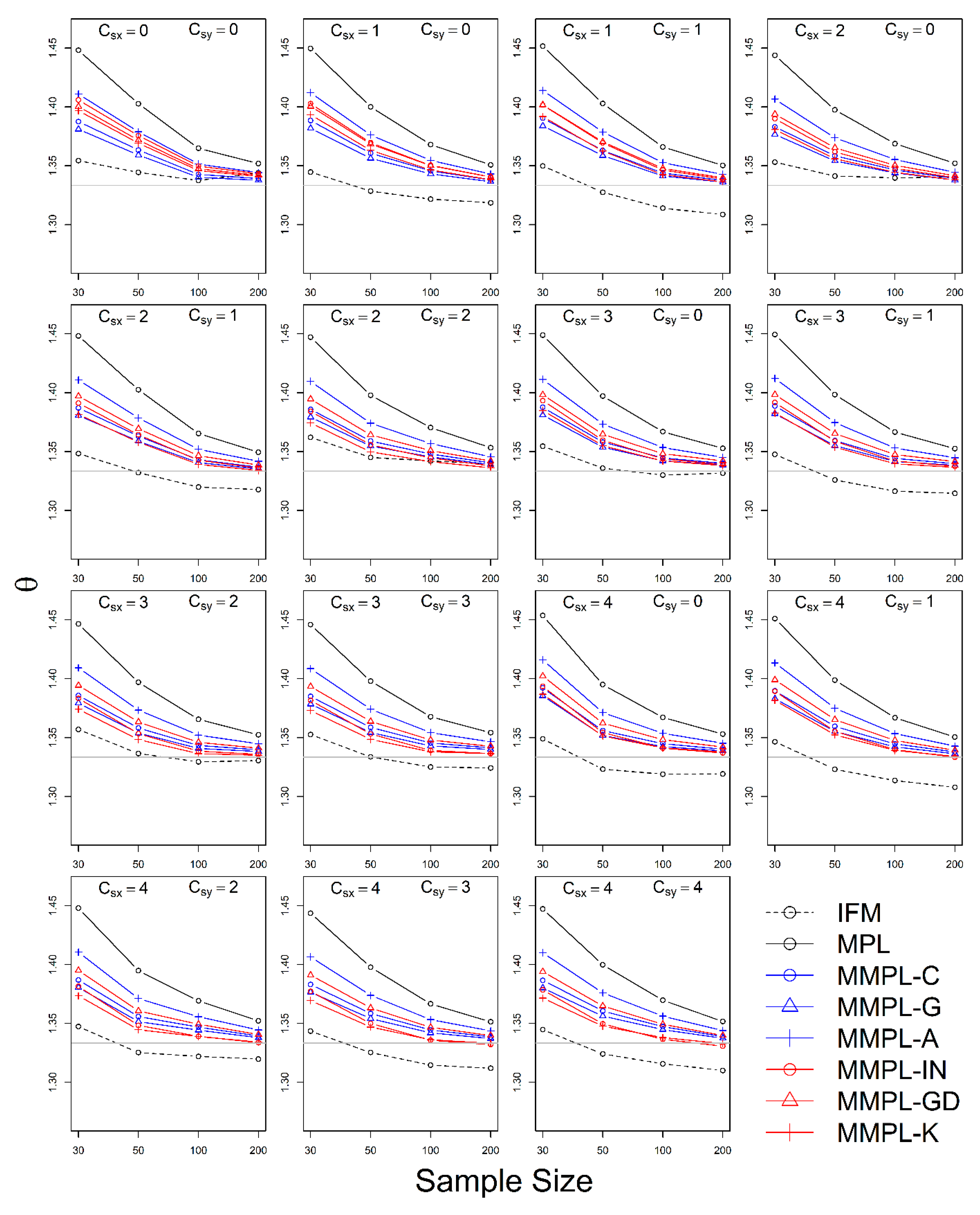
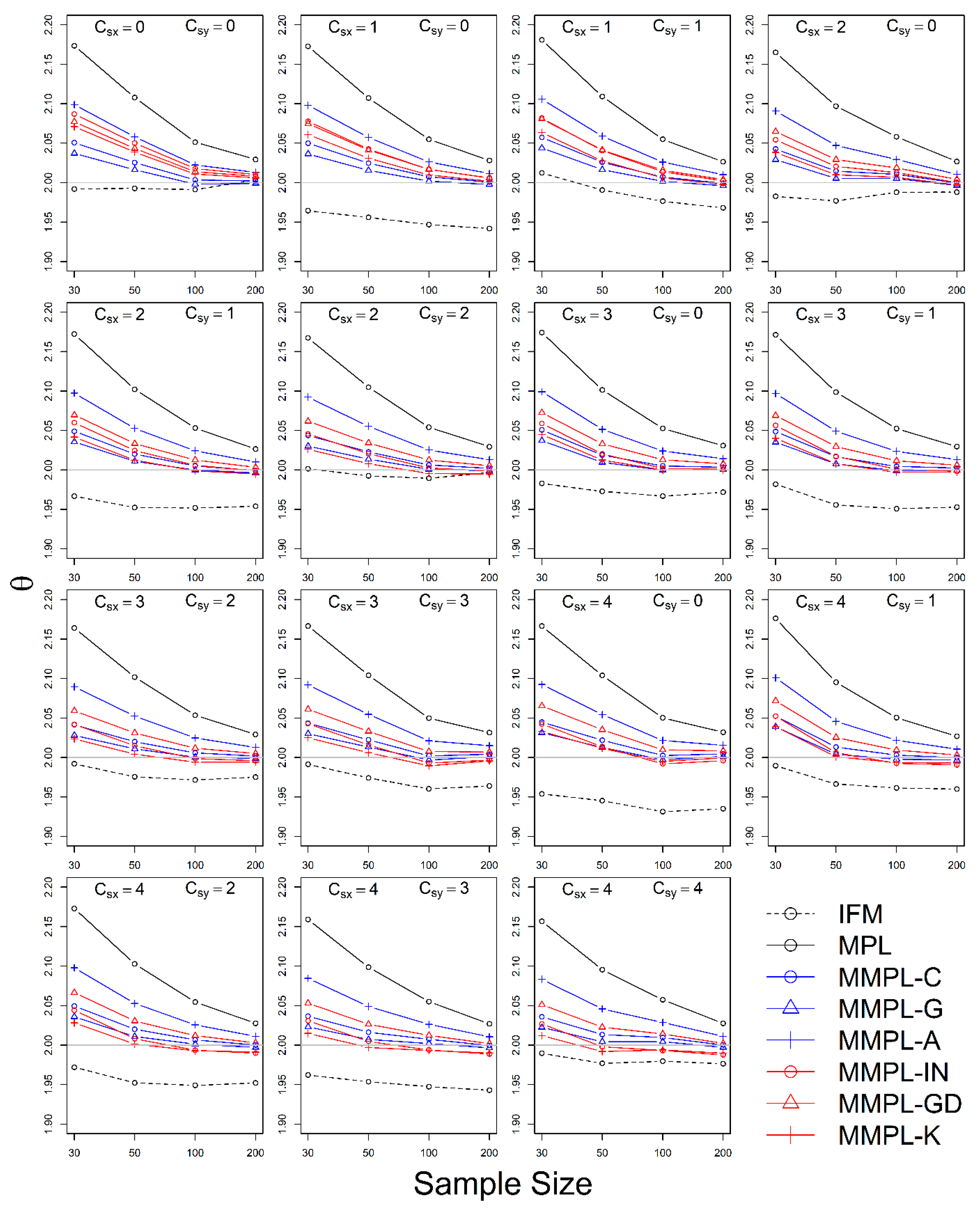
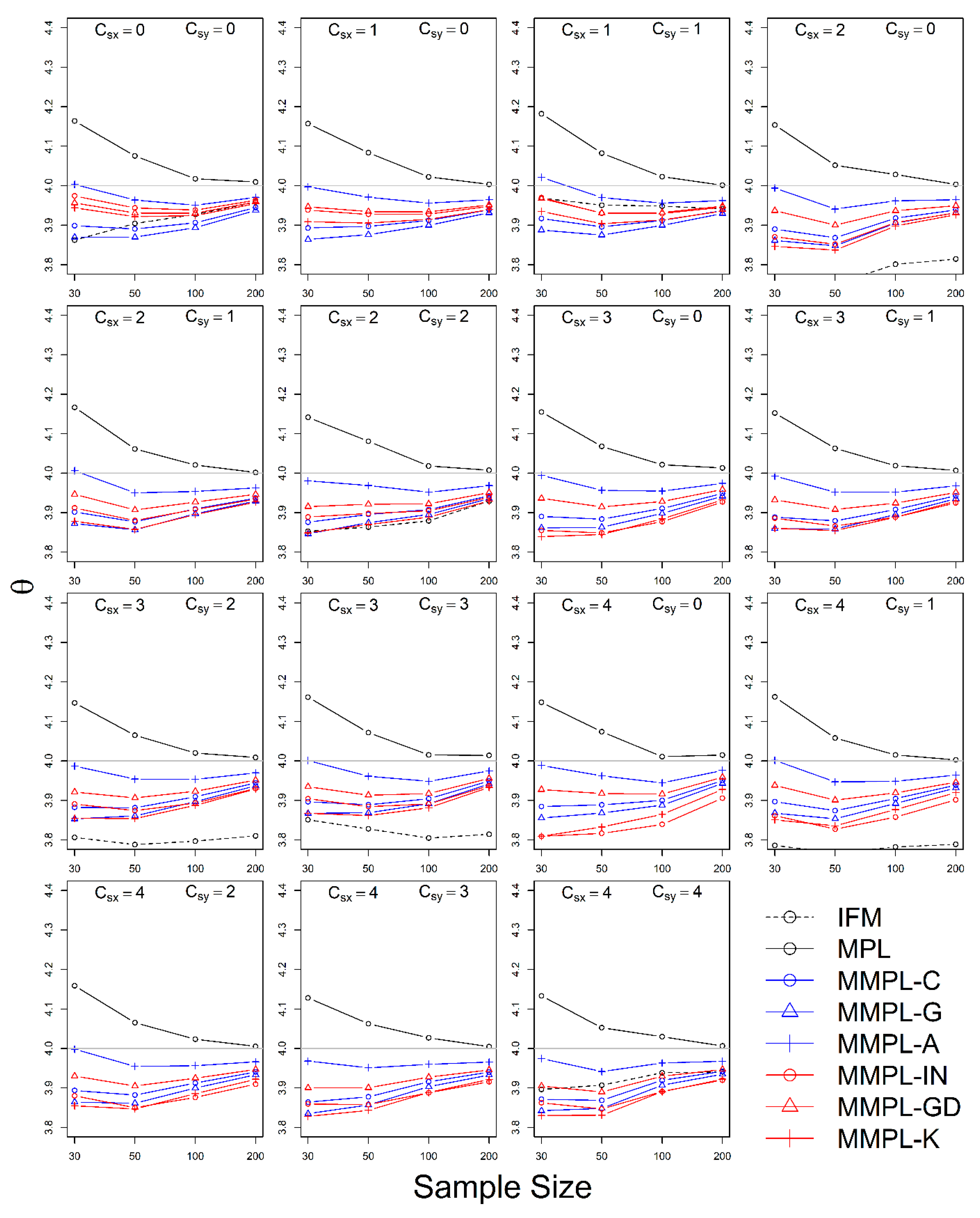
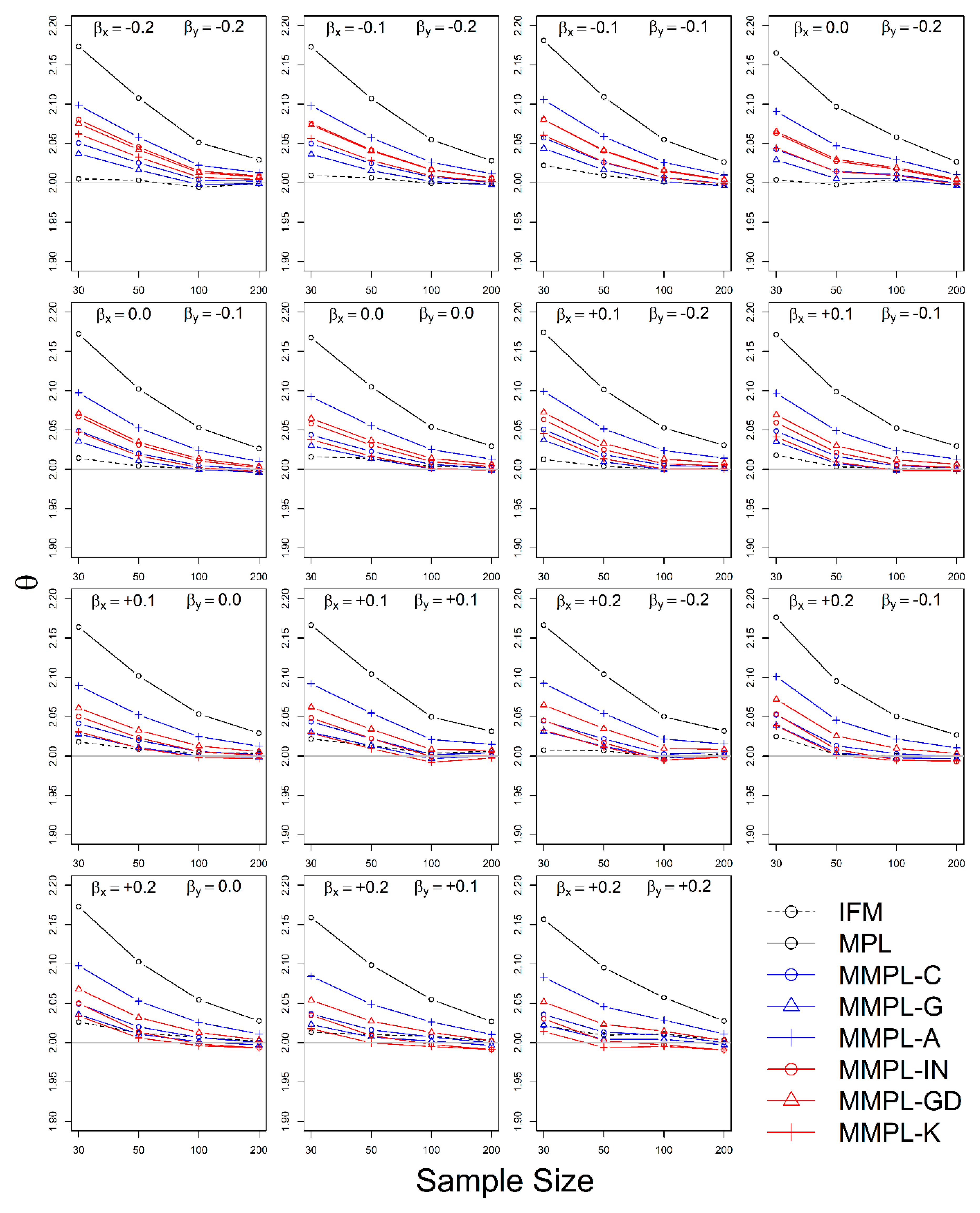
Figure 2, Figure 3 and Figure 4 present the averaged values of parameter estimates from 5000 sample sets for three dependence coefficients values (Figure 2: $\tau =$0.25; Figure 3: $\tau =$0.50; Figure 4: $\tau =$0.75). These three dependence coefficients are selected to describe the performance of the parameter estimation methods from weak to very strong correlation for illustration purposes. The results of these three correlation coefficients hold for the other cases with similar correlation coefficients. In Figure 2, Figure 3 and Figure 4, the $x$-axis indicates sample size and the gray line indicates the true value of the copula parameter. The black line is the MPL method, the dotted-line is the IFM method, the blue lines are the three MMPL methods without coefficient of skewness, and the red lines are the three MMPL methods with coefficient of skewness.

In general, for all combinations of $\tau =0.25$ and $\tau =0.50$ in Figure 2 and Figure 3, the parameter estimates by the MMPL methods are overall closest to the true value, while the MPL and IFM methods provide overestimation and underestimation for the copula parameter, respectively. The IFM method also fails to become closer to the true value of the copula parameter as sample size increases. In addition, for the combinations of $\tau =0.75$ in Figure 4, the MMPL methods underestimate the copula parameter, while the MPL method is closest to the true value as sample size increases. The MPL method shows a similar pattern for all combinations of different coefficients of skewness, while the MMPL methods do not. The IFM method generally provides the worst parameter estimates among all employed parameter estimation methods. In other words, the IFM method shows the severe underestimation of the copula parameter for many combinations of coefficient of skewness showing the parameter estimates below the limits of figures for eight combinations (1_0, 2_1, 3_0, 3_1, 4_0, 4_1, 4_2, and 4_3).

In the case of $\tau =0.25$ (Figure 2), the MMPL-K method generally leads to the best performance which provides the closest parameter estimates to the true value for 10 combinations in which the sum of the coefficients of skewness is larger than or equal to three, for example, 2_1, 2_2, 3_1, 3_2, 3_3, 4_0, 4_1, 4_2, 4_3, and 4_4 combinations. On the other hand, the MMPL-G method leads to the best performance for four combinations in which the sum of the coefficients of skewness is less than or equal to two, for example, 0_0, 1_0, 1_1, and 2_0 combinations. The parameter estimates by the IFM method are the closest to the true value when sample size is smaller than or equal to 50, but the IFM method converges to the true value of $\theta$ only when combinations of coefficient of skewness are 0_0, 2_0, 2_2, 3_0, and 3_2, while the other MPL and MMPL methods converge to the true value of $\theta$ for all combinations of coefficient of skewness. Note that the MMPL methods always show a better performance than that of the original MPL method for all combinations and sample sizes.

In the case of $\tau =0.50$ (Figure 3), the performance of parameter estimates from all methods show similar patterns to that obtained for the case of $\tau =0.25$. The MMPL-G method shows the best performance for four combinations in which the sum of the coefficients of skewness is smaller than or equal to 2 (0_0, 1_0, 1_1, and 2_0). Alternately, the MMPL-K method generally shows the best performance when the sum of the coefficients of skewness is larger than 4 even though it slightly underestimates the parameters when the sample size is larger than 50. The IFM method shows a worse performance than the previous case. The performance of the IFM method is only the best for a sample size of 30 in most combinations. As in the case of $\tau =0.25$, the MMPL methods show a better performance than that of the original MPL method for all combinations and sample sizes.

In the case of $\tau =0.75$ (Figure 4), in which random variables are unrealistically highly dependent, all the MMPL methods underestimate the copula parameter. The MMPL-A method leads to the best performance when sample size is less than or equal to 50, while the MPL method shows the best performance when sample size is larger than or equal to 100. The MMPL-A is generally the best MMPL method among the tested MMPL methods. As in the previous cases, the IFM method resulted in an underestimation for all coefficient of skewness combinations and shows very poor performance, especially for eight combinations (1_0, 2_1, 3_0, 3_1, 4_0, 4_1, 4_2, and 4_3) in which the parameter estimates lie below the lower limits of figures. The MPL method behaves well as sample size increases and shows the best performance when sample size is larger than or equal to 100.

4.2.2. Case of Known Marginal Distribution (GEV)

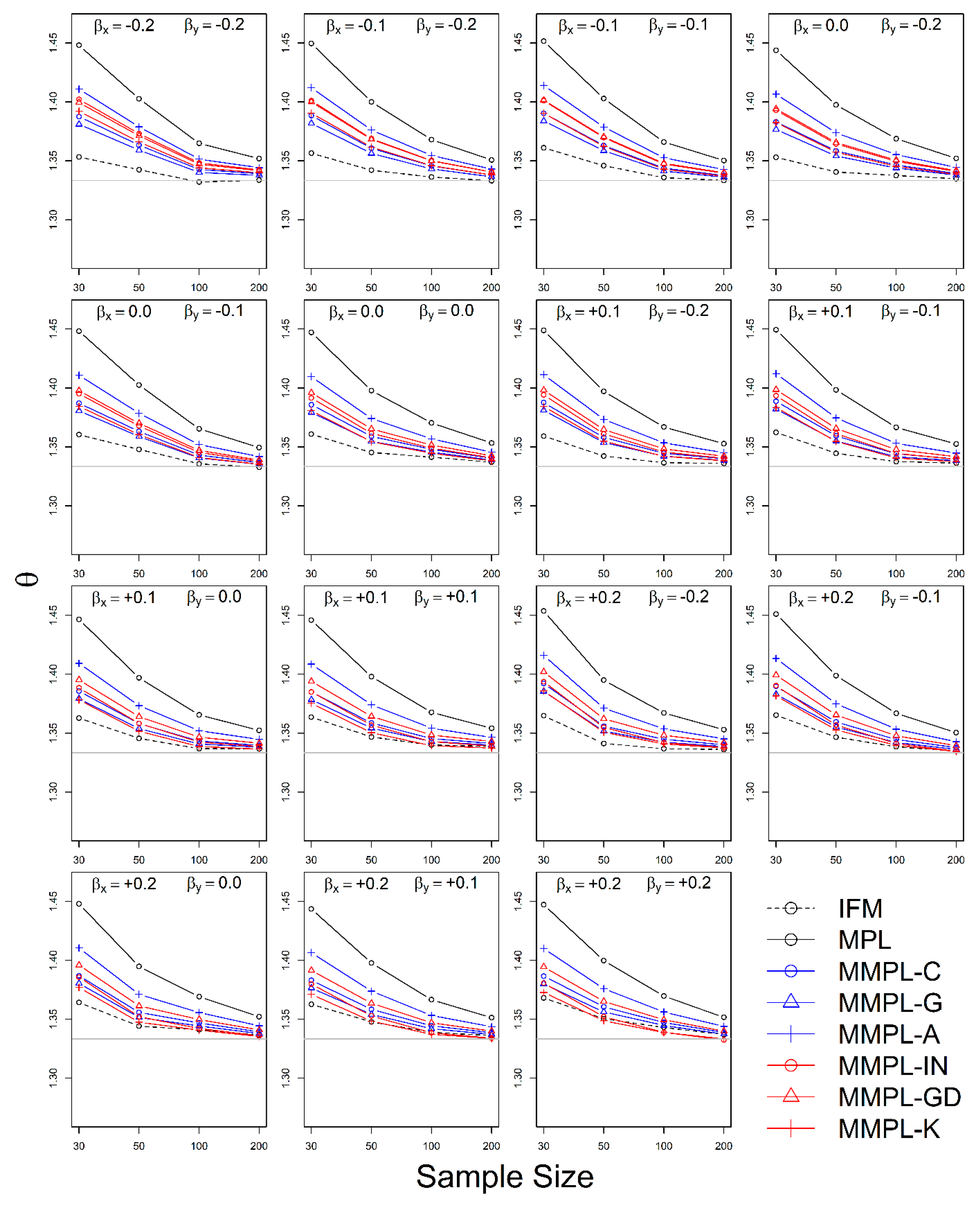
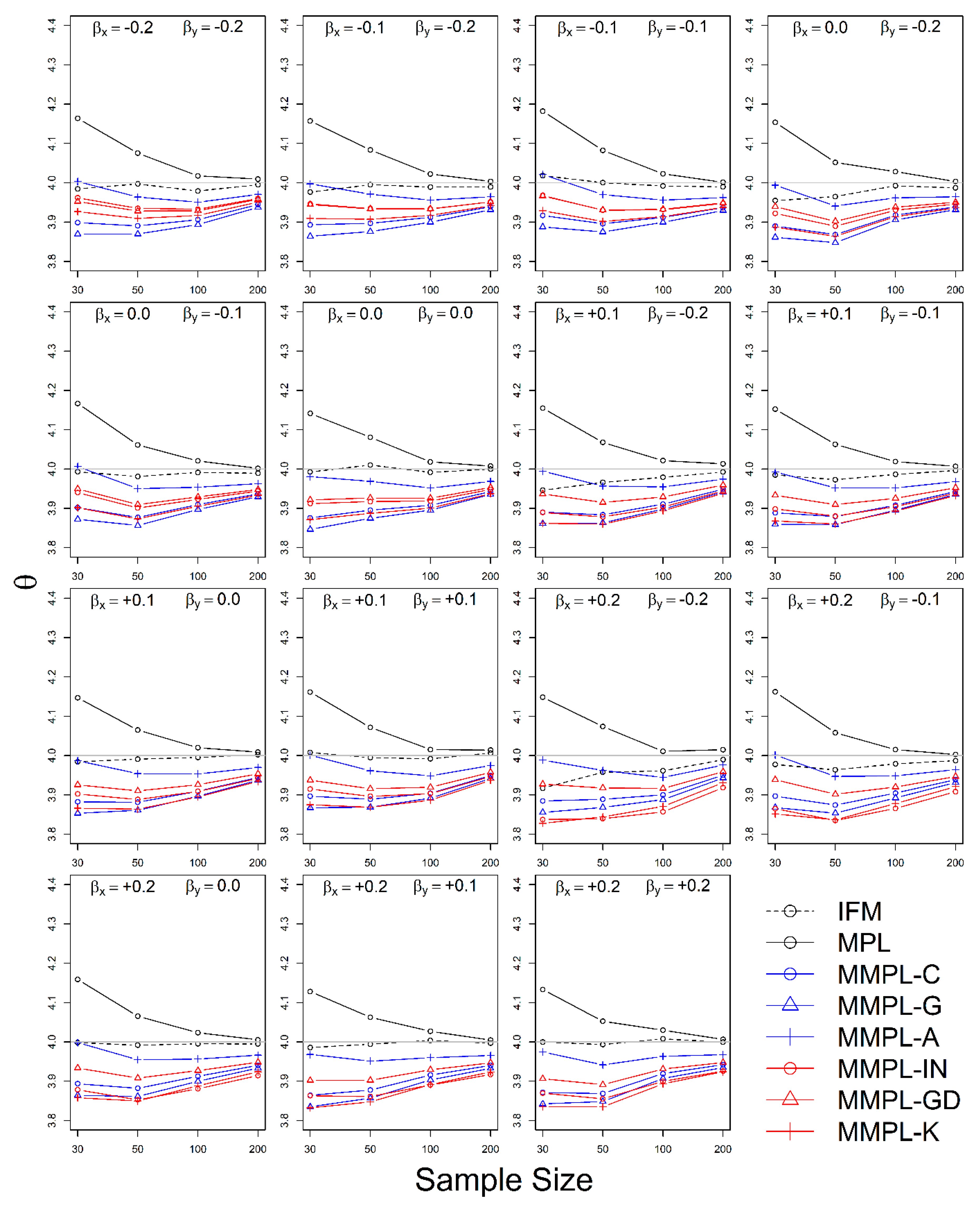
Figure 5, Figure 6 and Figure 7 present the averaged value of parameter estimates from 5000 sample sets for three values of dependence coefficients (Figure 5: $\tau =$0.25; Figure 6: $\tau =$0.50; Figure 7: $\tau =$0.75) as shown in the case of unknown marginal distribution. The performance of the IFM method is generally better than the MPL and MMPL methods. This is the expected result due to the assumption of the IFM method that the IFM method fits the copula model with a known marginal distribution model. The MMPL methods always provide better performance than the MPL method for the shape parameter combinations of $\tau =0.25$ and $\tau$= 0.50, while the MPL method shows better performance than the MMPL method when $\tau =0.75$ and larger sample size ($n\ge 100$).

In the case of $\tau =0.25$ (Figure 5), the IFM method shows the best performances for all shape parameter combinations except four combinations: 0.1_0.1, 0.2_0.0, 0.2_0.1, and 0.2_0.2. In these four combinations, the MMPL-K method shows to the best performance for large sample size, while the IFM method shows the best performance only for relatively small sample size ($n\le 50$). The IFM method generally shows the best performance when the sum of the shape parameters is smaller than or equal to 0.2, while the MMPL-K method shows the best performance when the sum of the shape parameters is larger than or equal to 0.2 and sample size is larger than 50. Among the MMPL methods, the MMPL-K method shows the best performance, except when the sum of the shape parameters is smaller than or equal to −0.1. For these combinations, the MMPL-G method shows slightly better performance than the MMPL-K method. Note that the original MPL method shows the worst performance for all combinations and sample sizes.

In the case of $\tau =0.50$ (Figure 6), the IFM method generally gives the closest parameter estimate to the true value for all shape parameter combinations, especially at small sample sizes. Similar to the case of unknown marginal distribution, overall performance of the MMPL-G and MMPL-K are better than the other tested MMPL methods. Even though the performance of the IFM method is greatly improved compared to the case of unknown marginal distribution, the MMPL methods provide closer parameter estimates to the true value than the IFM method for larger sample size and shape parameters. As in the case of $\tau =0.25$, the original MPL method shows the worst performance for all combinations.

In the case of $\tau =0.75$ (Figure 7), the IFM method generally provides better performance than the MPL and MMPL methods, which, respectively, overestimate and underestimate the copula parameter for all shape parameter combinations and sample sizes. The exception is that the MMPL-A method shows the best and second-best performance when sample sizes are 30 and 50, respectively. Among the MMPL methods, the MMPL-A method provides the best performance for all combinations of shape parameters and sample sizes even though it generally underestimates the copula parameter. As in case of unknown marginal distribution, the MPL method behaves well as sample size increases, and the performance is quite comparable to the IFM method, especially for large sample sizes.

5. Application

5.1. Data and Application Methodology

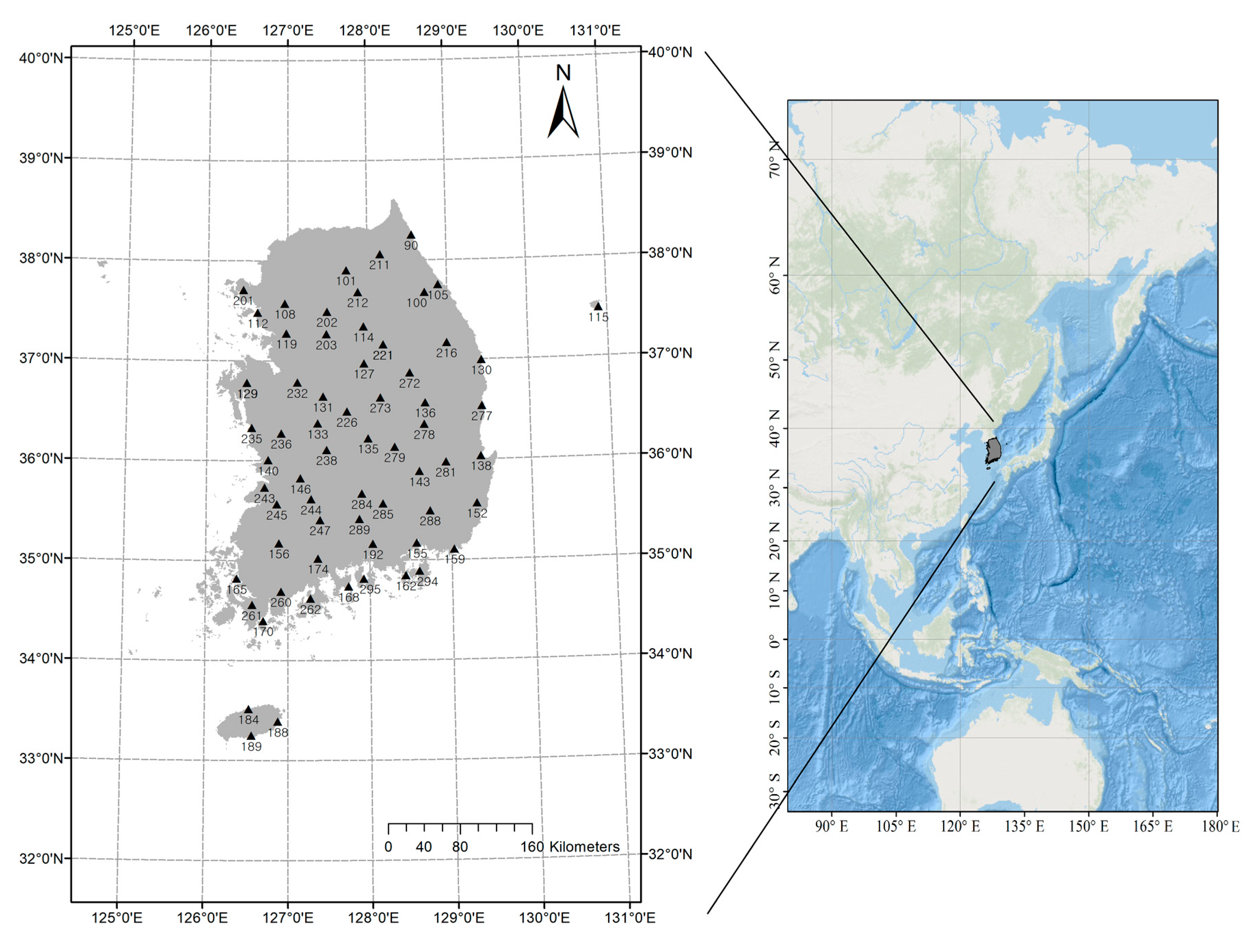
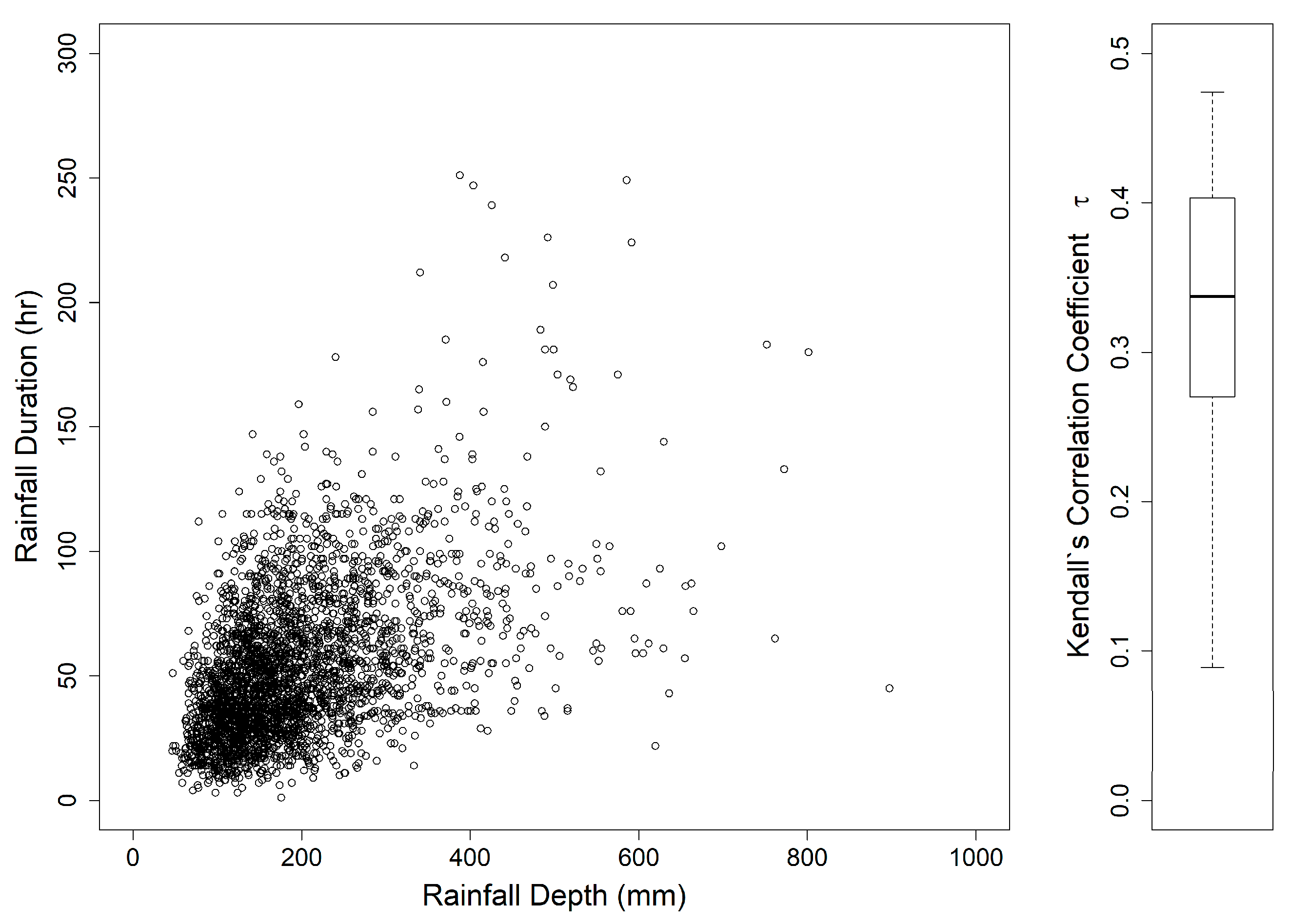
To investigate the difference between performances of the conventional estimation methods and the proposed estimation methods of the Gumbel copula for real hydrometeorological data, hourly rainfall data of 64 weather stations in South Korea were utilized. The locations of the weather stations are shown in Figure 8. The data were collected from the Korea Meteorological Association (https://data.kma.go.kr/cmmn/main.do), and the record lengths are from 32 to 56 years. Annual maximum volume (AMV) events were extracted from hourly recorded data, and then the rainfall volume and rainfall duration were used as random variables of bivariate Gumbel copula for each weather station. The scatter plot of all AMV events and the box-plot of Kendall’s tau ($\tau$) from 64 stations are illustrated in Figure 9. The rainfall volume and rainfall duration of AMV events are positively correlated. The range of the estimated Kendall’s tau ($\tau$) is from 0.089 to 0.474 for all 64 stations, in which there is no station with $\tau \ge 0.5$.

Of the 64 weather stations, the Seosan and Yeongwol stations were employed for the case study because their Kendall’s tau values are close to 0.25 (0.243) and 0.50 (0.474) in the simulation experiments, respectively, and the data length of the stations are 49 and 44 years, respectively. The coefficients of skewness of rainfall volume and rainfall duration are 1.80 and 1.46, respectively, for the Seosan station and 0.88 and 0.45 for the Yeongwol station, respectively.

To determine the type of marginal distribution for each variable, the chi-square goodness-of-fit test at 5% significance level ($\alpha =0.05$) and K-S distance statistic $D$ were employed. Five univariate probability distributions, namely GAM, GEV, GUM, GLO, and WBU, were used as marginal distribution candidates. For each variable of employed two stations,

Table 5. P-values of chi-square test and Kolmogorov-Smirnov distance statistics $D$ for each candidate distribution and variables of employed stations.

Station	Variable	Test	Statistic	GAM	GEV	GUM	GLO	WBU
Seosan	Volume	Chi-Square	p-value	0.034	0.727	0.053	0.071	0.004 *
		K-S	$D$	0.072	0.054	0.060	0.062	0.102
	Duration	Chi-Square	p-value	0.396	0.780	0.229	0.238	0.146
		K-S	$D$	0.102	0.060	0.108	0.108	0.106
Yeongwol	Volume	Chi-Square	p-value	0.895	0.837	0.818	0.825	0.822
		K-S	$D$	0.141	0.093	0.129	0.129	0.160
	Duration	Chi-Square	p-value	0.163	0.218	0.166	0.166	0.346
		K-S	$D$	0.108	0.099	0.105	0.104	0.098

* Rejected by chi-square test at 5% significance level ($\alpha$ = 0.05). Bolded value provides the most minimum K-S $D$ statistic from five marginal distribution candidates.

presents the p-values of the chi-square test and K-S distance statistics for each distribution candidate. For the Seosan station, the GEV distribution was selected for both marginal distributions. For the Yeongwol station, the GEV and WBU distributions were selected for rainfall volume and rainfall duration, respectively. The selected marginal distributions cannot be rejected by chi-square test and provide minimum K-S statistics among all distribution candidates.

5.2. Application Results

Table 6. Parameter estimates of annual maximum volume events for each parameter estimation methods.

Station	MPL	IFM	MMPL
			C	G	A	IN	GD	K
Seosan	1.352	1.290	1.309	1.305	1.326	1.304	1.315	1.296
Yeongwol	1.785	1.651	1.705	1.696	1.737	1.715	1.719	1.698

presents the estimates of the copula parameters from all employed parameter estimation methods. For the Seosan station, the parameter estimates by the MPL and IFM methods are 1.352 and 1.290, respectively. The parameter estimates of the six employed MMPL methods range from 1.296 to 1.326. For the Yeongwol station, the parameter estimates by the MPL and IFM methods are 1.785 and 1.651, respectively. The parameter estimates of the six employed MMPL methods range from 1.696 to 1.737.

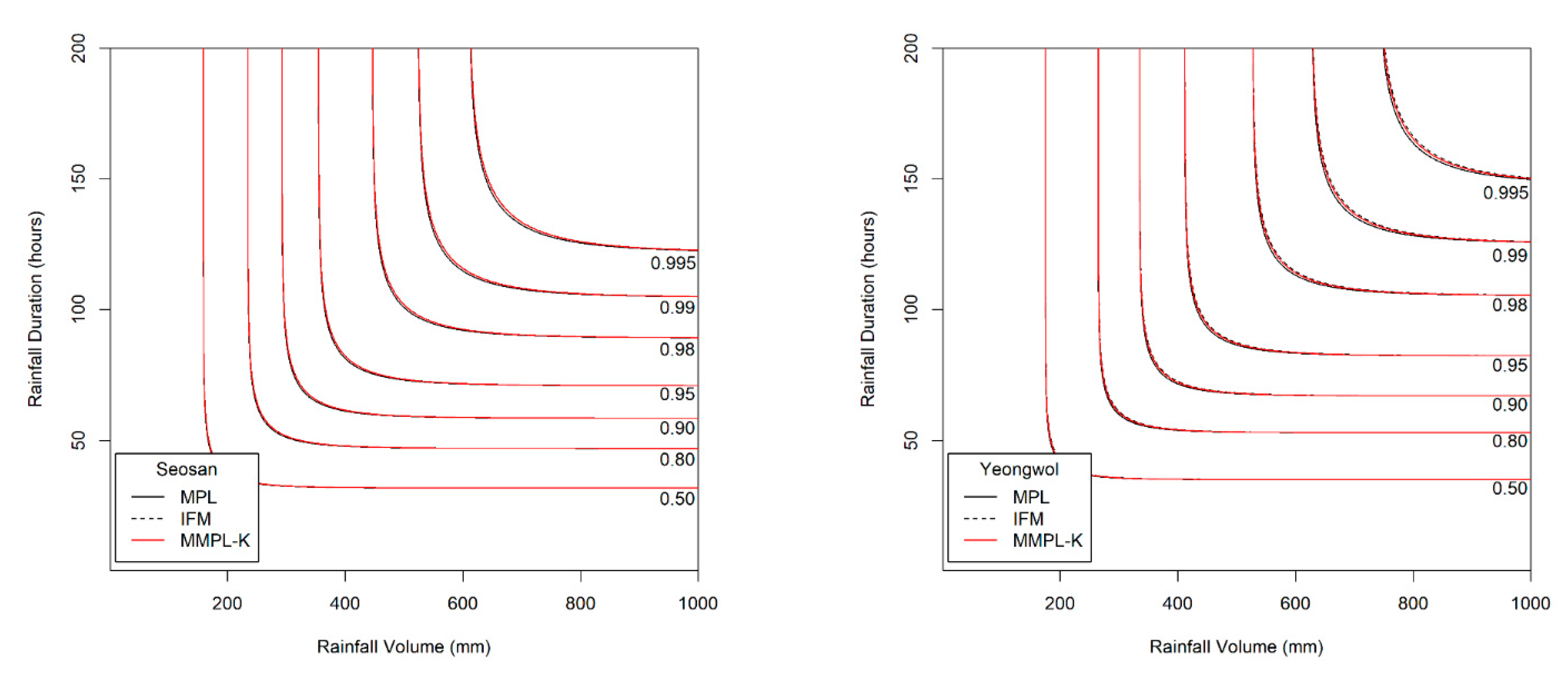
Joint probability of the estimated copula from three methods (MPL, IFM, and MMPL-K) are illustrated in Figure 10, which represents the joint occurrence probability of rainfall volume and rainfall duration. Since the MMPL-K method is most frequently selected to give the best performance from the results of the simulation experiment, it is illustrated in Figure 10 among the employed MMPL methods. As the probability increases, the differences among quantiles by the three methods increase. For example, a rainfall event with 523.6 mm of rainfall volume and 174.7 h rainfall duration corresponds to a 100 year return period, which corresponds to a 0.99 non-exceedance probability, for each marginal distribution of the Seosan station. The joint occurrence probabilities of the rainfall event (523.6 mm, 174.7 h) are 0.9833, 0.9829, and 0.9830 by the MPL, IFM, and MMPL-K methods, respectively. The joint occurrence probabilities correspond to 59.8, 58.5, and 58.8 years of return period by the MPL, IFM, and MMPL-K methods, respectively. Similar to the results of the Seosan station, a rainfall event with 627.0 mm of rainfall volume and 130.8 h rainfall duration corresponds to a 100 year return period for each marginal distribution at the Yeongwol station. The joint occurrence probabilities of the rainfall event (627.0 mm, 130.8 h) are 0.9853, 0.9848, and 0.9850 by the MPL, IFM, and MMPL-K methods, respectively. The joint occurrence probabilities correspond to 68.0, 65.8, and 66.7 years of return period by the MPL, IFM, and MMPL-K methods, respectively.

6. Discussion

The simulation experiment is designed by a variety of conditions, such as correlation, sample size, the unknown and known marginal distributions, and coefficients of skewness of data. The results of the simulation experiments showed, the proposed parameter estimation method led to improvements in the performances of parameter estimation for the copula model when margins follow skewed distribution models as compared to the conventional MPL method.

In the case of the unknown marginal distribution, the parameter estimate of the MMPL method led to the best performance, and the MPL and IFM methods follow. When marginal distribution information is unavailable, the MMPL and MPL methods have the advantage compared to the IFM method, because they fit the copula model regardless of the marginal distribution. Even though the IFM method shows better performance than the MPL and the MMPL methods at small sample size, the IFM method generally shows the worst performance for most combinations of coefficient of skewness. Moreover, it often shows severe underestimation of the parameter estimate for large sample sizes. In the case of known marginal distribution, the performance of the IFM method is expected to be better than the MPL and MMPL methods. The MMPL method provides the best performance in fitting the copula model in some cases with the large values of shape parameters and sample size based on the simulation experiments. The large value of the shape parameter can lead to large uncertainty in the parameter estimation of GEV distribution [57]. The performance of the MMPL method may be better than the IFM method for large shape parameters (large coefficient of skewness) because some employed plotting positions take coefficient of skewness into consideration.

The MMPL methods employed in this study are classified into two groups: adopting plotting position formula without coefficient of skewness and with coefficient of skewness. According to the results of simulation experiments, the MMPL-G method, which belongs to the former group, is considered the best parameter estimation method for data sets with small coefficients of skewness. The MMPL-K method, which belongs to the latter group, is considered the best MMPL method for data sets with large coefficients of skewness. The MMPL methods with plotting position formulas that consider coefficient of skewness might be a good choice when the sum of coefficients of skewness is larger than or equal to three based on the results of simulation experiments. Thus, the MMPL-K method would be the best alternative among the tested MMPL and MPL methods for fitting the copula model to the skewed data of hydrometeorological variables.

The MMPL method underestimates the copula parameter when the dependence of two variables is too strong. For example, when Kendall’s $\tau$ is 0.75 (see Figure 4 and Figure 7), the MPL and IFM methods provide good performances, except for the MMPL-A method, which, in this case, is considered the best method among the employed MMPL methods. Seventy-five hundredths is an unrealistically large coefficient at the applied 64 stations as shown in Figure 9. All Kendall’s $\tau$ are smaller than 0.5 at the applied 64 stations. For the skewed data, such as extreme precipitation and flood, the data sets with a very strong correlation may be infrequent. Thus, the MMPL method would be an alternative to the copula fitting methods for skewed data of hydrometeorological variables.

In this study, the bias is employed as a measure of accuracy compared to given true values of the copula parameter in the simulation experiment. For application of the real data sets, the parameter of population copula is unknown. Thus the bias may not be a good evaluation measure for real data sets. To overcome this drawback, goodness-of-fit tests are often used, and many of them examine goodness-of-fit by comparing empirical and estimated models. Because the empirical copula of goodness-of-fit tests, such as Kolmogorov- or Cramer-von Mises-type statistics, are based on the Weibull plotting position, the conventional goodness-of-fit tests are inappropriate for the MMPL methods. The goodness-of-fit tests should be modified or proposed for measuring goodness-of-fit of the copula model fitted by the MMPL method in the future.

7. Conclusions

In this study, a new parameter estimation method for the copula model was proposed. The proposed method is a modified version of the MPL method (MMPL). Six MMPL methods were proposed, and their performances and applicability were evaluated for the bivariate Gumbel copula model via the simulation experiments and case study to the extreme precipitation events. According to the results of the current study, the conclusions are as follows:

• The MMPL methods suggested in this paper prefers to estimate the parameters in a multivariate frequency analysis using the copula model for hydrometeorological data. The MMPL methods provide better performance than the original MPL method when the values of Kendall’s tau ($\tau$) are moderate ($\tau =0.25$ and $0.50$) in the simulation experiments regardless of unknown and known marginal distribution. However, for the case of $\tau =0.75$, which is very rare as shown in the applications, the original MPL method performs better than the MPL method, especially for large sample sizes showing convergence to the true value as the sample size increases. Among the MMPL methods, the MMPL-K and MMPL-G methods can be the best methods depending on the statistical characteristics of applied data.
• The original MPL method generally overestimates the parameters and shows the worst performance among the applied methods, but the parameter estimates converge to the true values as the sample size increases regardless of unknown and known marginal distributions and combinations of coefficient of skewness. However, this method shows comparably competitive to the best method, particularly when the sample size is large ($n\ge 100$) and $\tau =0.75$.
• The IFM method, as expected, shows the worst performances except for small sample size of 30 and underestimates the parameters severely as the Kendall’s tau increases in the case of unknown marginal distribution. However, in the case of known marginal distribution (GEV), the IFM method shows the best performance, while the MMPL-K method provides better performance than the IFM method when the sum of the shape parameters is larger than or equal to 0.2 in large sample sizes ($n\ge 50$) for the cases of moderate Kendall’s tau values. In addition, the IFM method generally performs the best even though Kendall’s tau is unrealistically large ($\tau =0.75$).

Finally, the suggested MMPL methods generally perform better than the original MPL method, except with very strong and unrealistic Kendall’s tau value ($\tau =0.75$), regardless of unknown and known marginal distributions. In addition, the MMPL methods perform marginally better than the IFM method when the sum of the shape parameters is larger than or equal to 0.2 in large sample sizes ($n\ge 50$), except $\tau =0.75$, even in the case of known marginal distribution. In conclusion, the MMPL-K and MMPL-G methods are appropriate methods of fitting the Gumbel copula model for the case of moderate Kendall’s tau values. Particularly, the MMPL-K method generally provides more accurate parameter estimates in the case of unknown marginal distribution when the sum of the coefficients of skewness is larger than or equal to three with $n>50$, and in the case of known marginal distribution when the sum of the shape parameters is larger than 0.2 with $n>50$.

References

1. Genest, C.; Favre, A.C. Everything you always wanted to know about copula modeling but were afraid to ask. J. Hydrol. Eng. 2007, 12, 347–368. [Google Scholar] [CrossRef]
2. Hashino, M. Formulation of the joint return period of two hydrologic variates associated with a Poisson process. J. Hydrosci. Hydraul. Eng. 1985, 3, 73–84. [Google Scholar]
3. Correia, F.N. Multivariate Partial Duration Series in Flood Risk Analysis. In Proceedings of the International Symposium on Flood Frequency and Risk Analyses, Louisiana State University, Baton Rouge, LA, USA, 14–17 May 1986; Singh, V.P., Ed.; Springer: Dordrecht, The Netherlands, 1987. [Google Scholar]
4. Goel, N.K.; De, M. Development of unbiased plotting position formula for General Extreme Value distributions. Stoch. Hydrol. Hydraul. 1993, 7, 1–13. [Google Scholar] [CrossRef]
5. Singh, K.; Singh, V.P. Derivation of bivariate probability density functions with exponential marginals. Stoch. Hydrol. Hydraul. 1991, 5, 55–68. [Google Scholar] [CrossRef]
6. Yue, S. Joint probability distribution of annual maximum storm peaks and amounts as represented by daily rainfalls. Hydrol. Sci. J. 2000, 45, 315–326. [Google Scholar] [CrossRef]
7. Grimaldi, S.; Serinaldi, F. Design hyetograph analysis with 3-copula function. Hydrol. Sci. J. 2006, 51, 223–238. [Google Scholar] [CrossRef]
8. Kao, S.C.; Govindaraju, R.S. A bivariate frequency analysis of extreme rainfall with implications for design. J. Geophys. Res. Atmos. 2007, 112, D13119. [Google Scholar] [CrossRef]
9. Jun, C.; Qin, X.; Gan, T.Y.; Tung, Y.K.; De Michele, C. Bivariate frequency analysis of rainfall intensity and duration for urban stormwater infrastructure design. J. Hydrol. 2017, 553, 374–383. [Google Scholar] [CrossRef]
10. Reddy, M.J.; Singh, V.P. Multivariate modeling of droughts using copulas and meta-heuristic methods. Stoch. Environ. Res. Risk Assess. 2014, 28, 475–489. [Google Scholar] [CrossRef]
11. Chang, J.; Li, Y.; Wang, Y.; Yuan, M. Copula-based drought risk assessment combined with an integrated index in the Wei River Basin, China. J. Hydrol. 2016, 540, 824–834. [Google Scholar] [CrossRef]
12. Tosunoglu, F.; Kisi, O. Joint modelling of annual maximum drought severity and corresponding duration. J. Hydrol. 2016, 543, 406–422. [Google Scholar] [CrossRef]
13. Riberio, A.F.S.; Russo, A.; Gouveia, C.M.; Páscoa, P.; Pires, C.A.L. Probabilistic modeling of the dependence between rainfed crops and drought hazard. Nat. Hazards Earth Syst. Sci. 2019, 19, 2795–2809. [Google Scholar] [CrossRef] [Green Version]
14. Vazifehkhah, S.; Tosunoglu, F.; Kahya, E. Bivariate risk analysis of droughts using a nonparametric multivariate standardized drought index and copulas. J. Hydrol. Eng. 2019, 24, 05019006. [Google Scholar] [CrossRef]
15. Zhang, Q.; Chen, Y.D.; Chen, X.; Li, J. Copula-based analysis of hydrological extremes and implications of hydrological behaviors in the Pearl River Basin, China. J. Hydrol. Eng. 2011, 16, 598–607. [Google Scholar] [CrossRef]
16. Chen, Y.D.; Zhang, Q.; Xiao, M.; Singh, V.P. Evaluation of risk of hydrological droughts by the trivariate Plackett copula in the East River basin (China). Nat. Hazards 2013, 68, 529–547. [Google Scholar] [CrossRef]
17. Salvadori, G.; De Michele, C. Multivariate real-time assessment of droughts via copula-based multi-site Hazard Trajectories and Fans. J. Hydrol. 2015, 526, 101–115. [Google Scholar] [CrossRef]
18. Xu, K.; Yang, D.; Xu, X.; Lei, H. Copula based drought frequency analysis considering the spatio-temporal variability in Southwest China. J. Hydrol. 2015, 527, 630–640. [Google Scholar] [CrossRef]
19. Zhang, L.; Singh, V.P. Bivariate flood frequency analysis using the copula method. J. Hydrol. Eng. 2006, 11, 150–164. [Google Scholar] [CrossRef]
20. Sraj, M.; Bezak, N.; Brilly, M. Bivariate flood frequency analysis using the copula function: A case study of the Litija station on the Sava River. Hydrol. Process. 2015, 29, 225–238. [Google Scholar] [CrossRef]
21. Genest, C.; Rivest, L.P. Statistical inference procedures for bivariate Archimedean copulas. J. Am. Stat. Assoc. 1993, 88, 1034–1043. [Google Scholar] [CrossRef]
22. Genest, C.; Ghoudi, K.; Rivest, L.P. A semiparametric estimation procedure of dependence parameters in multivariate families of distributions. Biometrika 1995, 82, 543–552. [Google Scholar] [CrossRef]
23. Folland, C.; Anderson, C. Estimating changing extremes using empirical ranking methods. J. Clim. 2002, 15, 2954–2960. [Google Scholar] [CrossRef]
24. Joe, H.; Xu, J.J. The Estimation Method of Inference Functions for Margins for Multivariate Models; Technical Report No. 166; Department of Statistics, University of British Columbia: Vancouver, BC, Canada, 1996. [Google Scholar]
25. Parent, E.; Favre, A.C.; Bernier, J.; Perreault, L. Copula models for frequency analysis what can be learned from a Bayesian perspective? Adv. Water Resour. 2014, 63, 91–103. [Google Scholar] [CrossRef]
26. Kwon, H.H.; Lall, U. A copula-based nonstationary frequency analysis for the 2012–2015 drought in California. Water Resour. Res. 2016, 52, 5662–5675. [Google Scholar] [CrossRef] [Green Version]
27. Sadegh, M.; Ragno, E.; Agha Kouchak, A. Multivariate Copula Analysis Toolbox (MvCAT): Describing dependence and underlying uncertainty using a Bayesian framework. Water Resour. Res. 2017, 53, 5166–5183. [Google Scholar] [CrossRef]
28. Brahimi, B.; Chebana, F.; Necir, A. Copula representation of bivariate L-moments: A new estimation method for multiparameter two-dimensional copula models. Statistics 2015, 49, 497–521. [Google Scholar] [CrossRef]
29. Sklar, A. Fonctions de répartition à n dimensions et leurs marges. Publ. Inst. Stat. Univ. Paris 1959, 8, 229–231. [Google Scholar]
30. Zhang, L. Multivariate Hydrological Frequency Analysis and Risk Mapping. Ph.D. Thesis, Agricultural and Mechanical College, Louisiana State University, Baton Rouge, LA, USA, 2005. [Google Scholar]
31. Corbella, S.; Stretch, D.D. Simulating a multivariate sea storm using Archimedean copulas. Coast. Eng. 2013, 76, 68–78. [Google Scholar] [CrossRef]
32. Xing, Z.; Yan, D.; Zhang, C.; Wang, G.; Zhang, D. Spatial Characterization and Bivariate Frequency Analysis of Precipitation and Runoff in the Upper Huai River Basin, China. Water Resour. Manag. 2015, 29, 3291–3304. [Google Scholar] [CrossRef]
33. Balistrocchi, M.; Orlandini, S.; Ranzi, R.; Bacchi, B. Copula-Based Modeling of Flood Control Reservoirs. Water Resour. Res. 2017, 53, 9883–9900. [Google Scholar] [CrossRef]
34. Li, H.; Wang, D.; Singh, V.P.; Wang, Y.; Wu, J.; Wu, J.; Liu, J.; Zou, Y.; He, R.; Zhang, J. Non-stationary frequency analysis of annual extreme rainfall volume and intensity using Archimedean copulas: A case study in eastern China. J. Hydrol. 2019, 571, 114–131. [Google Scholar] [CrossRef]
35. Nelsen, R.B. An Introduction to Copulas, 2nd ed.; Springer: New York, NY, USA, 2006. [Google Scholar]
36. Gudendorf, G.; Segers, J. Extreme-Value Copulas. In Copula Theory and Its Applications, 1st ed.; Jaworski, P., Durante, F., Härdle, W., Rychlik, T., Eds.; Springer: Berlin/Heidelberg, Germany, 2010; Volume 198, pp. 127–145. [Google Scholar]
37. Favre, A.C.; El Adlouni, S.; Perreault, L.; Thiémonge, N.; Bobée, B. Multivariate hydrological frequency analysis using copulas. Water Resour. Res. 2004, 40. [Google Scholar] [CrossRef] [Green Version]
38. Fu, G.; Butler, D. Copula-based frequency analysis of overflow and flooding in urban drainage systems. J. Hydrol. 2014, 510, 49–58. [Google Scholar] [CrossRef] [Green Version]
39. Bezak, N.; Šraj, M.; Mikoš, M. Copula-based IDF curves and empirical rainfall thresholds for flash floods and rainfall-induced landslides. J. Hydrol. 2016, 541, 272–284. [Google Scholar] [CrossRef]
40. Tu, X.; Du, Y.; Singh, V.P.; Chen, X.; Zhao, Y.; Ma, M.; Li, K.; Wu, H. Bivariate Design of Hydrological Droughts and Their Alterations under a Changing Environment. J. Hydrol. Eng. 2019, 24, 04019015. [Google Scholar] [CrossRef]
41. Salvadori, G.; De Michele, C. Multivariate Extreme Value Methods. In Extremes in a Changing Climate. Detection, Analysis and Uncertainty, 1st ed.; AghaKouchak, A., Easterling, D., Hsu, K., Schubert, S., Sorooshian, S., Eds.; Springer: Dordrecht, The Netherlands, 2013; pp. 115–162. [Google Scholar]
42. Zhang, J.; Ng, W.L. Exact Maximum Likelihood Estimation for Copula Models. Working Papers 038. Research Report of COMISEF, 2010. Available online: http://comisef.eu/files/wps038.pdf (accessed on 10 March 2020).
43. Weiß, G. Copula parameter estimation by maximum-likelihood and minimum-distance estimators: A simulation study. Comput. Stat. 2011, 26, 31–54. [Google Scholar] [CrossRef]
44. Makonen, L. Plotting Position in Extreme Value Analysis. J. Appl. Meteor. Climatol. 2006, 45, 334–340. [Google Scholar] [CrossRef]
45. Cook, N. Comments on “Plotting Positions in Extreme Value Analysis”. J. Appl. Meteor. Climatol. 2011, 50, 255–266. [Google Scholar] [CrossRef]
46. Yahaya, A.S.; Nor, N.M.; Jali, N.R.M.; Ramli, N.A.; Ahmad, F.; Ul-Saufie, Z. Determination of the Probability Plotting Position for Type I Extreme Value Distribution. J. Appl. Sci. 2012, 12, 1501–1506. [Google Scholar]
47. Gringorten, I.I. A plotting rule for extreme probability paper. J. Geophys. Res. 1963, 68, 813–814. [Google Scholar] [CrossRef]
48. Cunnane, C. Unbiased plotting positions—A review. J. Hydrol. 1978, 37, 205–222. [Google Scholar] [CrossRef]
49. Adamowski, K. Plotting Formula for Flood Frequency. J. Am. Water Resour. Assoc. 1981, 17, 197–202. [Google Scholar] [CrossRef]
50. In-na, N.; Nyuyen, V.T.V. An unbiased plotting position formula for the general extreme value distribution. J. Hydrol. 1989, 106, 193–209. [Google Scholar] [CrossRef]
51. Goel, N.K.; Seth, S.M.; Chandra, S. Multivariate modeling of flood flows. J. Hydraul. Eng. 1998, 124, 146–155. [Google Scholar] [CrossRef]
52. Kim, S.; Shin, H.; Joo, K.; Heo, J.H. Development of plotting position for the general extreme value distribution. J. Hydrol. 2012, 475, 259–269. [Google Scholar] [CrossRef]
53. Griffiths, G.A. A theoretically based Wakeby distribution for annual flood series. Hydrol. Sci. J. 1989, 34, 231–248. [Google Scholar] [CrossRef] [Green Version]
54. Rahman, A.; Zaman, M.A.; Haddad, K.; El Adlouni, S.; Zhang, C. Applicability of Wakeby distribution in flood frequency analysis: A case study for eastern Australia. Hydrol. Process. 2014, 29, 602–614. [Google Scholar] [CrossRef]
55. Landwehr, J.M.; Matalas, N.C.; Wallis, J.R. Estimation of parameters and quantiles of Wakeby Distributions: 1. Known lower bounds. Water Resour. Res. 1979, 15, 1361–1372. [Google Scholar] [CrossRef]
56. Jenkinson, A.F. The frequency distribution of the annual maximum (or minimum) values of meteorological elements. Q. J. R. Meteorol. Soc. 1955, 81, 158–171. [Google Scholar] [CrossRef]
57. Martins, E.S.; Stedinger, J.R. Generalized maximum-likelihood generalized extreme-value quantile estimators for hydrologic data. Water Resour. Res. 2000, 36, 737–744. [Google Scholar] [CrossRef]
Figure 1. The simulation cases and process of each parameter estimation method. GEV = generalized extreme value; IFM = Inference Functions for Margins.
Water 12 01182 g001
Figure 2. Averaged value of copula parameter estimates from 5000 sample sets for each coefficient of skewness ( γ x , γ y ) combination of the case assuming unknown marginal distribution ( τ = 0.25 , θ = 1.33 ).
Water 12 01182 g002
Figure 3. Averaged value of copula parameter estimates from 5000 sample sets for each coefficient of skewness ( γ x , γ y ) combination of the case assuming unknown marginal distribution ( τ = 0.50 , θ = 2.0 ).
Water 12 01182 g003
Figure 4. Averaged value of copula parameter estimates from 5000 sample sets for each coefficient of skewness ( γ x , γ y ) combination of the case assuming unknown marginal distribution ( τ = 0.75 , θ = 4.0 ).
Water 12 01182 g004
Figure 5. Averaged value of copula parameter estimates from 5000 sample sets for each shape parameter ( β x , β y ) combination of the case assuming known marginal distribution ( τ = 0.25 , θ = 1.33 ).
Water 12 01182 g005
Figure 6. Averaged value of copula parameter estimates from 5000 sample sets for each shape parameter ( β x , β y ) combination of the case assuming known marginal distribution ( τ = 0.50 , θ = 2.0 ).
Water 12 01182 g006
Figure 7. Averaged value of copula parameter estimates from 5000 sample sets for each shape parameter ( β x , β y ) combination of the case assuming known marginal distribution ( τ = 0.75 , θ = 4.0 ).
Water 12 01182 g007
Figure 8. Locations of weather stations and their station numbers, South Korea (two stations marked with bold (129, 221) are employed to illustrate joint probability contour plot).
Water 12 01182 g008
Figure 9. Scatter plot of annual maximum volume events from all 64 stations and box-plot of Kendall’s correlation coefficient τ.
Water 12 01182 g009
Figure 10. Joint occurrence probability of rainfall volume and rainfall duration from three parameter estimation methods of the Seosan and Yeongwol stations.
Water 12 01182 g010