Modified Maximum Pseudo Likelihood Method of Copula Parameter Estimation for Skewed Hydrometeorological Data


Abstract
1. Introduction
2. Theoretical Background
2.1. Copula Model
2.2. Conventional Parameter Estimation Methods
2.2.1. Inference Function for Margin (IFM)
2.2.2. Maximum Pseudo-Likelihood Method (MPL)
3. Modified Maximum Pseudo-Likelihood Method (MMPL)
4. Simulation Experiment
4.1. Simulation Design
4.1.1. Case of Unknown Marginal Distribution
4.1.2. Case of Known Marginal Distribution
4.1.3. Finding Appropriate Marginal Distribution
4.2. Simulation Results
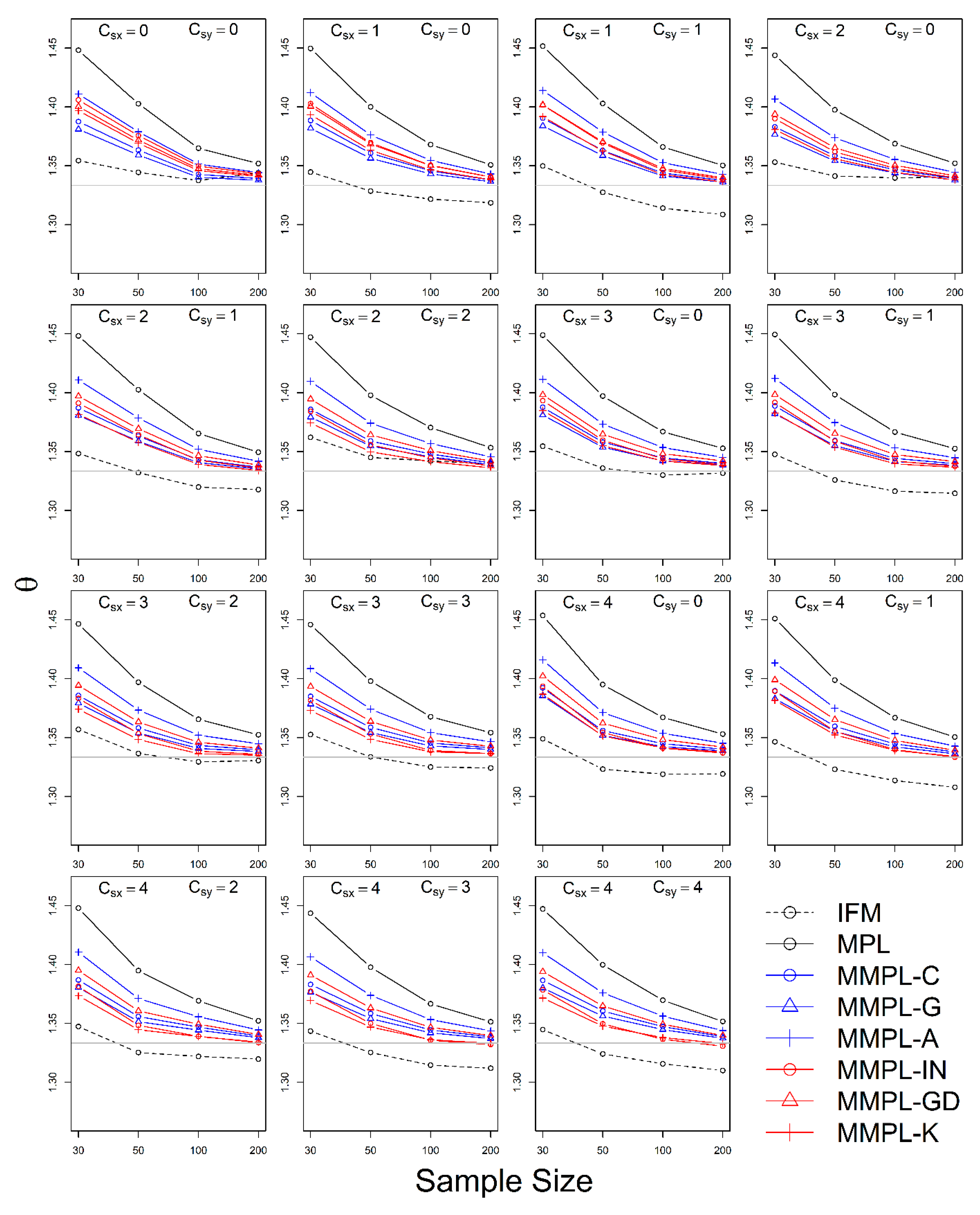
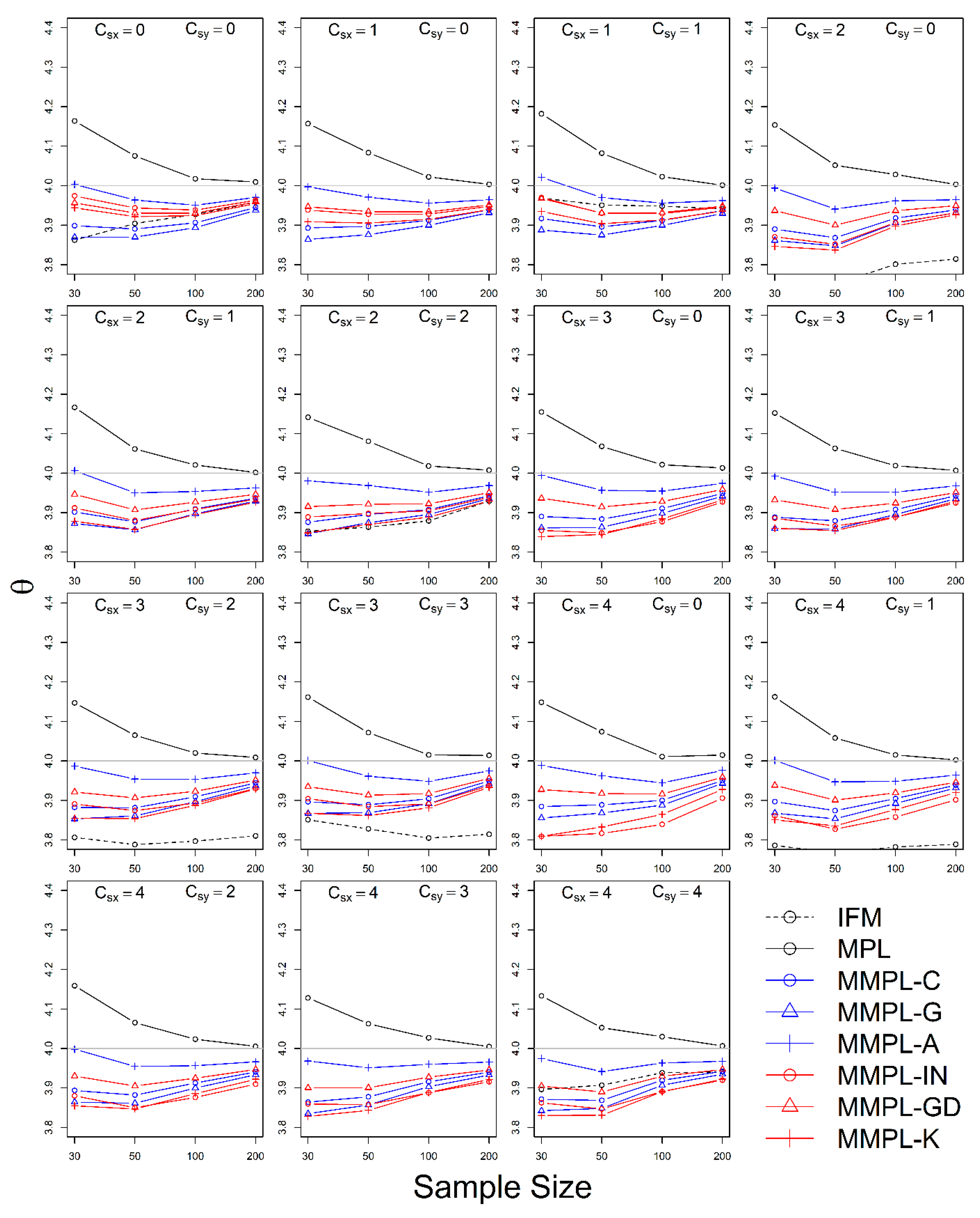
4.2.1. Case of Unknown Marginal Distribution (Wakeby)
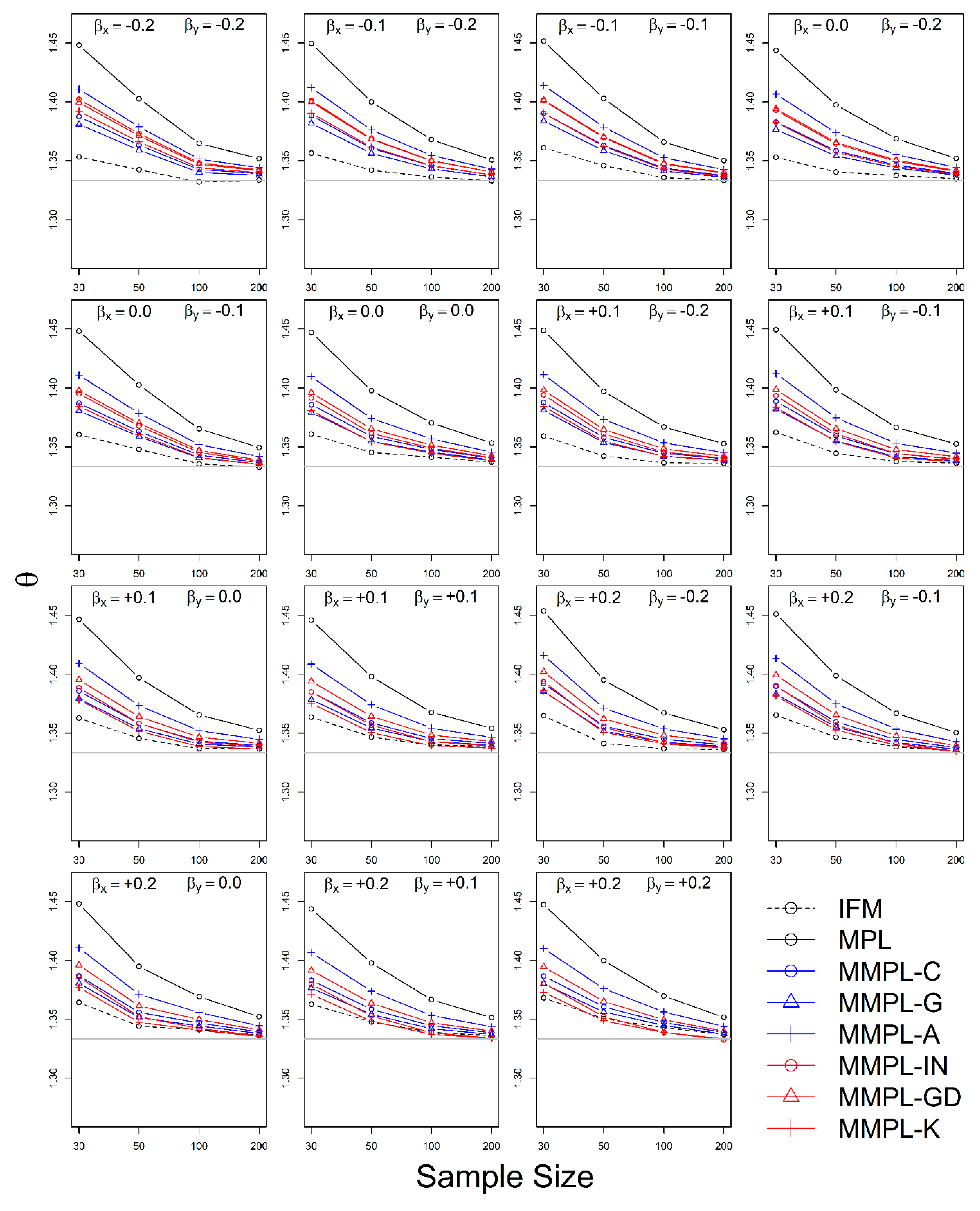
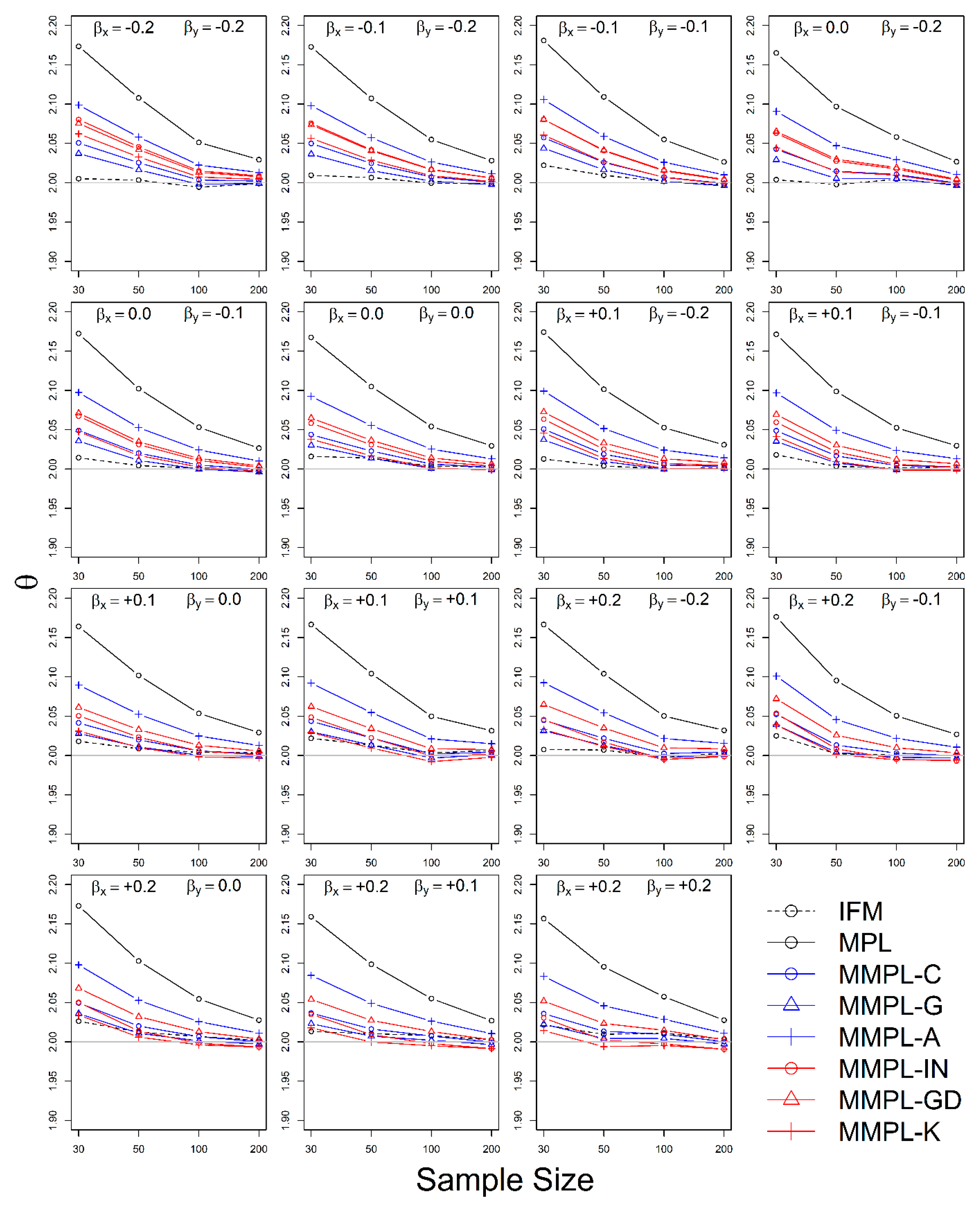
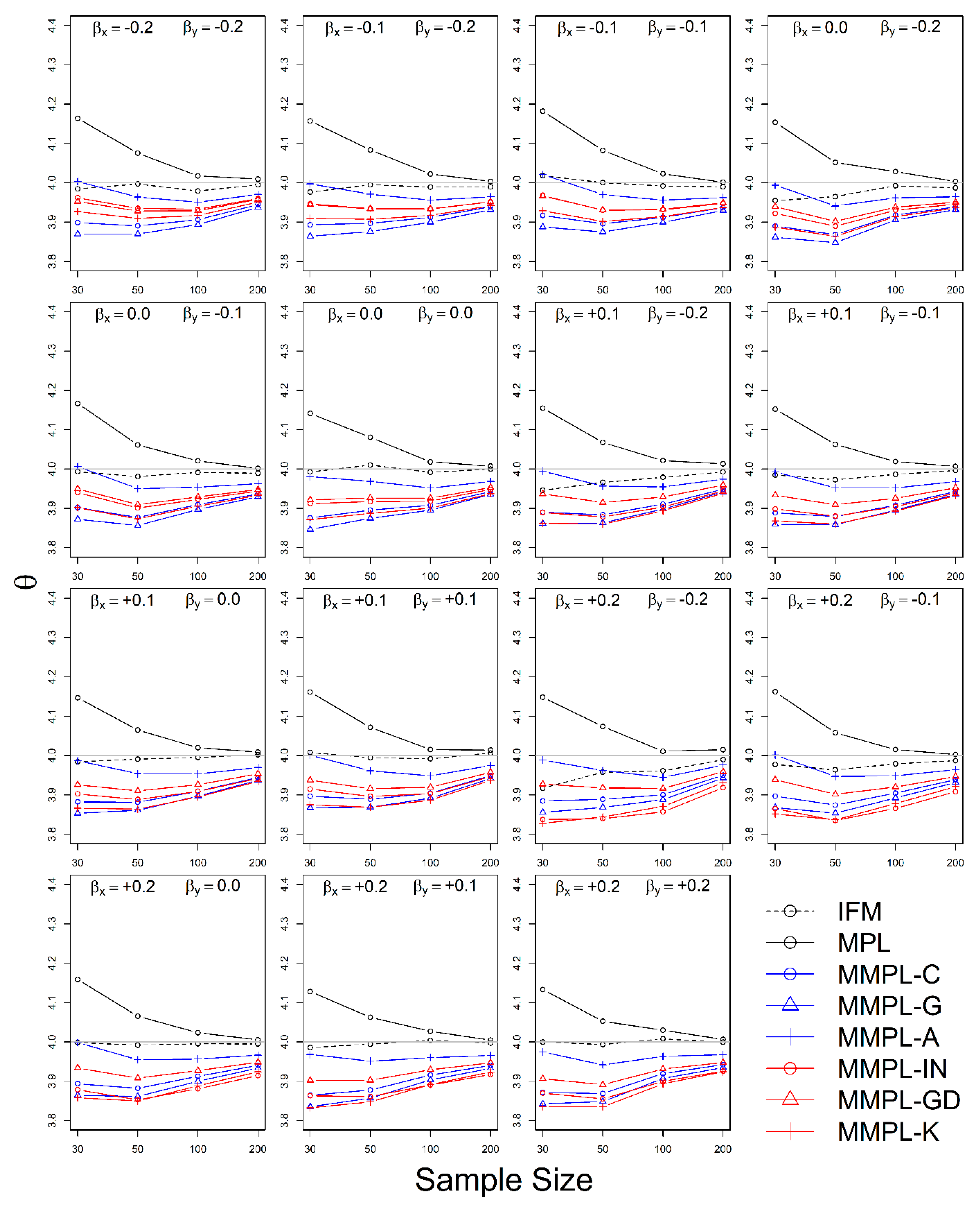
4.2.2. Case of Known Marginal Distribution (GEV)
5. Application
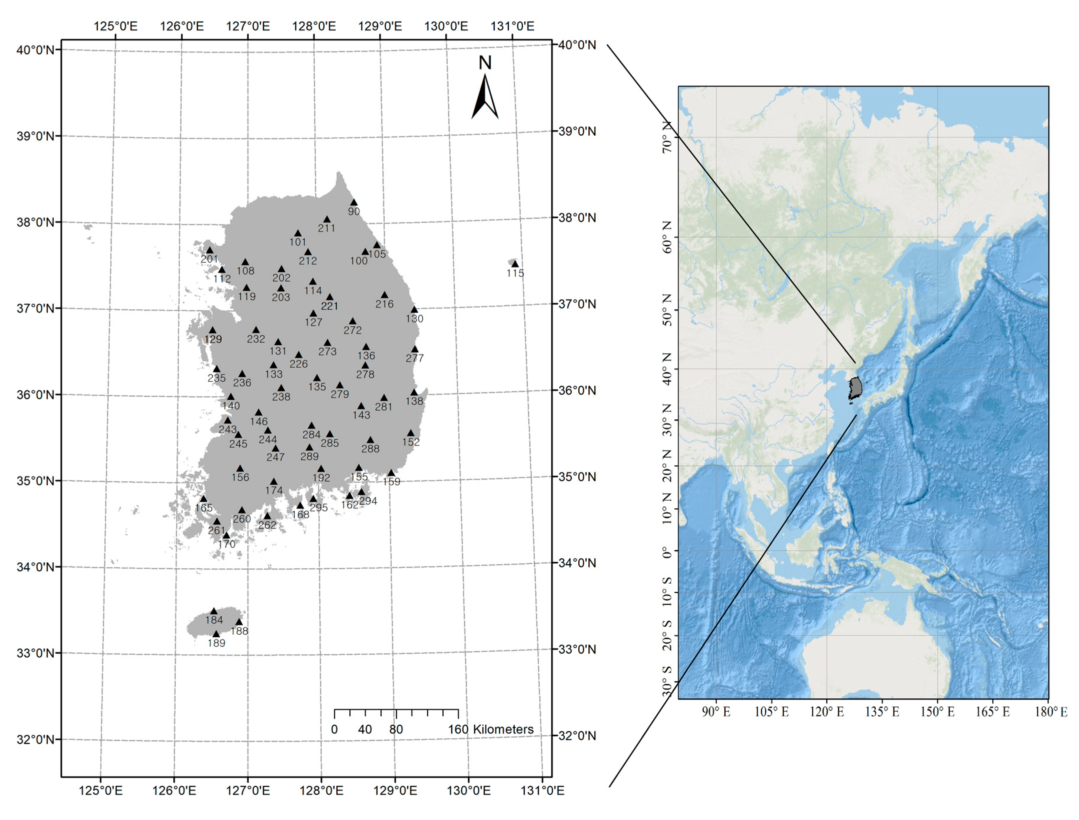
5.1. Data and Application Methodology
5.2. Application Results
6. Discussion
7. Conclusions
- The MMPL methods suggested in this paper prefers to estimate the parameters in a multivariate frequency analysis using the copula model for hydrometeorological data. The MMPL methods provide better performance than the original MPL method when the values of Kendall’s tau () are moderate ( and ) in the simulation experiments regardless of unknown and known marginal distribution. However, for the case of , which is very rare as shown in the applications, the original MPL method performs better than the MPL method, especially for large sample sizes showing convergence to the true value as the sample size increases. Among the MMPL methods, the MMPL-K and MMPL-G methods can be the best methods depending on the statistical characteristics of applied data.
- The original MPL method generally overestimates the parameters and shows the worst performance among the applied methods, but the parameter estimates converge to the true values as the sample size increases regardless of unknown and known marginal distributions and combinations of coefficient of skewness. However, this method shows comparably competitive to the best method, particularly when the sample size is large () and .
- The IFM method, as expected, shows the worst performances except for small sample size of 30 and underestimates the parameters severely as the Kendall’s tau increases in the case of unknown marginal distribution. However, in the case of known marginal distribution (GEV), the IFM method shows the best performance, while the MMPL-K method provides better performance than the IFM method when the sum of the shape parameters is larger than or equal to 0.2 in large sample sizes () for the cases of moderate Kendall’s tau values. In addition, the IFM method generally performs the best even though Kendall’s tau is unrealistically large ().
Author Contributions
Funding
Conflicts of Interest
References
- Genest, C.; Favre, A.C. Everything you always wanted to know about copula modeling but were afraid to ask. J. Hydrol. Eng. 2007, 12, 347–368. [Google Scholar] [CrossRef]
- Hashino, M. Formulation of the joint return period of two hydrologic variates associated with a Poisson process. J. Hydrosci. Hydraul. Eng. 1985, 3, 73–84. [Google Scholar]
- Correia, F.N. Multivariate Partial Duration Series in Flood Risk Analysis. In Proceedings of the International Symposium on Flood Frequency and Risk Analyses, Louisiana State University, Baton Rouge, LA, USA, 14–17 May 1986; Singh, V.P., Ed.; Springer: Dordrecht, The Netherlands, 1987. [Google Scholar]
- Goel, N.K.; De, M. Development of unbiased plotting position formula for General Extreme Value distributions. Stoch. Hydrol. Hydraul. 1993, 7, 1–13. [Google Scholar] [CrossRef]
- Singh, K.; Singh, V.P. Derivation of bivariate probability density functions with exponential marginals. Stoch. Hydrol. Hydraul. 1991, 5, 55–68. [Google Scholar] [CrossRef]
- Yue, S. Joint probability distribution of annual maximum storm peaks and amounts as represented by daily rainfalls. Hydrol. Sci. J. 2000, 45, 315–326. [Google Scholar] [CrossRef]
- Grimaldi, S.; Serinaldi, F. Design hyetograph analysis with 3-copula function. Hydrol. Sci. J. 2006, 51, 223–238. [Google Scholar] [CrossRef]
- Kao, S.C.; Govindaraju, R.S. A bivariate frequency analysis of extreme rainfall with implications for design. J. Geophys. Res. Atmos. 2007, 112, D13119. [Google Scholar] [CrossRef]
- Jun, C.; Qin, X.; Gan, T.Y.; Tung, Y.K.; De Michele, C. Bivariate frequency analysis of rainfall intensity and duration for urban stormwater infrastructure design. J. Hydrol. 2017, 553, 374–383. [Google Scholar] [CrossRef]
- Reddy, M.J.; Singh, V.P. Multivariate modeling of droughts using copulas and meta-heuristic methods. Stoch. Environ. Res. Risk Assess. 2014, 28, 475–489. [Google Scholar] [CrossRef]
- Chang, J.; Li, Y.; Wang, Y.; Yuan, M. Copula-based drought risk assessment combined with an integrated index in the Wei River Basin, China. J. Hydrol. 2016, 540, 824–834. [Google Scholar] [CrossRef]
- Tosunoglu, F.; Kisi, O. Joint modelling of annual maximum drought severity and corresponding duration. J. Hydrol. 2016, 543, 406–422. [Google Scholar] [CrossRef]
- Riberio, A.F.S.; Russo, A.; Gouveia, C.M.; Páscoa, P.; Pires, C.A.L. Probabilistic modeling of the dependence between rainfed crops and drought hazard. Nat. Hazards Earth Syst. Sci. 2019, 19, 2795–2809. [Google Scholar] [CrossRef]
- Vazifehkhah, S.; Tosunoglu, F.; Kahya, E. Bivariate risk analysis of droughts using a nonparametric multivariate standardized drought index and copulas. J. Hydrol. Eng. 2019, 24, 05019006. [Google Scholar] [CrossRef]
- Zhang, Q.; Chen, Y.D.; Chen, X.; Li, J. Copula-based analysis of hydrological extremes and implications of hydrological behaviors in the Pearl River Basin, China. J. Hydrol. Eng. 2011, 16, 598–607. [Google Scholar] [CrossRef]
- Chen, Y.D.; Zhang, Q.; Xiao, M.; Singh, V.P. Evaluation of risk of hydrological droughts by the trivariate Plackett copula in the East River basin (China). Nat. Hazards 2013, 68, 529–547. [Google Scholar] [CrossRef]
- Salvadori, G.; De Michele, C. Multivariate real-time assessment of droughts via copula-based multi-site Hazard Trajectories and Fans. J. Hydrol. 2015, 526, 101–115. [Google Scholar] [CrossRef]
- Xu, K.; Yang, D.; Xu, X.; Lei, H. Copula based drought frequency analysis considering the spatio-temporal variability in Southwest China. J. Hydrol. 2015, 527, 630–640. [Google Scholar] [CrossRef]
- Zhang, L.; Singh, V.P. Bivariate flood frequency analysis using the copula method. J. Hydrol. Eng. 2006, 11, 150–164. [Google Scholar] [CrossRef]
- Sraj, M.; Bezak, N.; Brilly, M. Bivariate flood frequency analysis using the copula function: A case study of the Litija station on the Sava River. Hydrol. Process. 2015, 29, 225–238. [Google Scholar] [CrossRef]
- Genest, C.; Rivest, L.P. Statistical inference procedures for bivariate Archimedean copulas. J. Am. Stat. Assoc. 1993, 88, 1034–1043. [Google Scholar] [CrossRef]
- Genest, C.; Ghoudi, K.; Rivest, L.P. A semiparametric estimation procedure of dependence parameters in multivariate families of distributions. Biometrika 1995, 82, 543–552. [Google Scholar] [CrossRef]
- Folland, C.; Anderson, C. Estimating changing extremes using empirical ranking methods. J. Clim. 2002, 15, 2954–2960. [Google Scholar] [CrossRef]
- Joe, H.; Xu, J.J. The Estimation Method of Inference Functions for Margins for Multivariate Models; Technical Report No. 166; Department of Statistics, University of British Columbia: Vancouver, BC, Canada, 1996. [Google Scholar]
- Parent, E.; Favre, A.C.; Bernier, J.; Perreault, L. Copula models for frequency analysis what can be learned from a Bayesian perspective? Adv. Water Resour. 2014, 63, 91–103. [Google Scholar] [CrossRef]
- Kwon, H.H.; Lall, U. A copula-based nonstationary frequency analysis for the 2012–2015 drought in California. Water Resour. Res. 2016, 52, 5662–5675. [Google Scholar] [CrossRef]
- Sadegh, M.; Ragno, E.; Agha Kouchak, A. Multivariate Copula Analysis Toolbox (MvCAT): Describing dependence and underlying uncertainty using a Bayesian framework. Water Resour. Res. 2017, 53, 5166–5183. [Google Scholar] [CrossRef]
- Brahimi, B.; Chebana, F.; Necir, A. Copula representation of bivariate L-moments: A new estimation method for multiparameter two-dimensional copula models. Statistics 2015, 49, 497–521. [Google Scholar] [CrossRef]
- Sklar, A. Fonctions de répartition à n dimensions et leurs marges. Publ. Inst. Stat. Univ. Paris 1959, 8, 229–231. [Google Scholar]
- Zhang, L. Multivariate Hydrological Frequency Analysis and Risk Mapping. Ph.D. Thesis, Agricultural and Mechanical College, Louisiana State University, Baton Rouge, LA, USA, 2005. [Google Scholar]
- Corbella, S.; Stretch, D.D. Simulating a multivariate sea storm using Archimedean copulas. Coast. Eng. 2013, 76, 68–78. [Google Scholar] [CrossRef]
- Xing, Z.; Yan, D.; Zhang, C.; Wang, G.; Zhang, D. Spatial Characterization and Bivariate Frequency Analysis of Precipitation and Runoff in the Upper Huai River Basin, China. Water Resour. Manag. 2015, 29, 3291–3304. [Google Scholar] [CrossRef]
- Balistrocchi, M.; Orlandini, S.; Ranzi, R.; Bacchi, B. Copula-Based Modeling of Flood Control Reservoirs. Water Resour. Res. 2017, 53, 9883–9900. [Google Scholar] [CrossRef]
- Li, H.; Wang, D.; Singh, V.P.; Wang, Y.; Wu, J.; Wu, J.; Liu, J.; Zou, Y.; He, R.; Zhang, J. Non-stationary frequency analysis of annual extreme rainfall volume and intensity using Archimedean copulas: A case study in eastern China. J. Hydrol. 2019, 571, 114–131. [Google Scholar] [CrossRef]
- Nelsen, R.B. An Introduction to Copulas, 2nd ed.; Springer: New York, NY, USA, 2006. [Google Scholar]
- Gudendorf, G.; Segers, J. Extreme-Value Copulas. In Copula Theory and Its Applications, 1st ed.; Jaworski, P., Durante, F., Härdle, W., Rychlik, T., Eds.; Springer: Berlin/Heidelberg, Germany, 2010; Volume 198, pp. 127–145. [Google Scholar]
- Favre, A.C.; El Adlouni, S.; Perreault, L.; Thiémonge, N.; Bobée, B. Multivariate hydrological frequency analysis using copulas. Water Resour. Res. 2004, 40. [Google Scholar] [CrossRef]
- Fu, G.; Butler, D. Copula-based frequency analysis of overflow and flooding in urban drainage systems. J. Hydrol. 2014, 510, 49–58. [Google Scholar] [CrossRef]
- Bezak, N.; Šraj, M.; Mikoš, M. Copula-based IDF curves and empirical rainfall thresholds for flash floods and rainfall-induced landslides. J. Hydrol. 2016, 541, 272–284. [Google Scholar] [CrossRef]
- Tu, X.; Du, Y.; Singh, V.P.; Chen, X.; Zhao, Y.; Ma, M.; Li, K.; Wu, H. Bivariate Design of Hydrological Droughts and Their Alterations under a Changing Environment. J. Hydrol. Eng. 2019, 24, 04019015. [Google Scholar] [CrossRef]
- Salvadori, G.; De Michele, C. Multivariate Extreme Value Methods. In Extremes in a Changing Climate. Detection, Analysis and Uncertainty, 1st ed.; AghaKouchak, A., Easterling, D., Hsu, K., Schubert, S., Sorooshian, S., Eds.; Springer: Dordrecht, The Netherlands, 2013; pp. 115–162. [Google Scholar]
- Zhang, J.; Ng, W.L. Exact Maximum Likelihood Estimation for Copula Models. Working Papers 038. Research Report of COMISEF, 2010. Available online: http://comisef.eu/files/wps038.pdf (accessed on 10 March 2020).
- Weiß, G. Copula parameter estimation by maximum-likelihood and minimum-distance estimators: A simulation study. Comput. Stat. 2011, 26, 31–54. [Google Scholar] [CrossRef]
- Makonen, L. Plotting Position in Extreme Value Analysis. J. Appl. Meteor. Climatol. 2006, 45, 334–340. [Google Scholar] [CrossRef]
- Cook, N. Comments on “Plotting Positions in Extreme Value Analysis”. J. Appl. Meteor. Climatol. 2011, 50, 255–266. [Google Scholar] [CrossRef]
- Yahaya, A.S.; Nor, N.M.; Jali, N.R.M.; Ramli, N.A.; Ahmad, F.; Ul-Saufie, Z. Determination of the Probability Plotting Position for Type I Extreme Value Distribution. J. Appl. Sci. 2012, 12, 1501–1506. [Google Scholar]
- Gringorten, I.I. A plotting rule for extreme probability paper. J. Geophys. Res. 1963, 68, 813–814. [Google Scholar] [CrossRef]
- Cunnane, C. Unbiased plotting positions—A review. J. Hydrol. 1978, 37, 205–222. [Google Scholar] [CrossRef]
- Adamowski, K. Plotting Formula for Flood Frequency. J. Am. Water Resour. Assoc. 1981, 17, 197–202. [Google Scholar] [CrossRef]
- In-na, N.; Nyuyen, V.T.V. An unbiased plotting position formula for the general extreme value distribution. J. Hydrol. 1989, 106, 193–209. [Google Scholar] [CrossRef]
- Goel, N.K.; Seth, S.M.; Chandra, S. Multivariate modeling of flood flows. J. Hydraul. Eng. 1998, 124, 146–155. [Google Scholar] [CrossRef]
- Kim, S.; Shin, H.; Joo, K.; Heo, J.H. Development of plotting position for the general extreme value distribution. J. Hydrol. 2012, 475, 259–269. [Google Scholar] [CrossRef]
- Griffiths, G.A. A theoretically based Wakeby distribution for annual flood series. Hydrol. Sci. J. 1989, 34, 231–248. [Google Scholar] [CrossRef][Green Version]
- Rahman, A.; Zaman, M.A.; Haddad, K.; El Adlouni, S.; Zhang, C. Applicability of Wakeby distribution in flood frequency analysis: A case study for eastern Australia. Hydrol. Process. 2014, 29, 602–614. [Google Scholar] [CrossRef]
- Landwehr, J.M.; Matalas, N.C.; Wallis, J.R. Estimation of parameters and quantiles of Wakeby Distributions: 1. Known lower bounds. Water Resour. Res. 1979, 15, 1361–1372. [Google Scholar] [CrossRef]
- Jenkinson, A.F. The frequency distribution of the annual maximum (or minimum) values of meteorological elements. Q. J. R. Meteorol. Soc. 1955, 81, 158–171. [Google Scholar] [CrossRef]
- Martins, E.S.; Stedinger, J.R. Generalized maximum-likelihood generalized extreme-value quantile estimators for hydrologic data. Water Resour. Res. 2000, 36, 737–744. [Google Scholar] [CrossRef]


| Formula | Equation |
|---|---|
| MMPL-C (Cunnane) [47] | |
| MMPL-G (Gringorten) [48] | |
| MMPL-A (Adamowski) [49] | |
| MMPL-IN (In-na and Nguyen) [50] | |
| MMPL-GD (Goel and De) [51] | |
| MMPL-K (Kim) [52] |
| No. | Parameters | Statistics | ||||||||
|---|---|---|---|---|---|---|---|---|---|---|
| CV | ||||||||||
| 1 | 0 | 1 | 2.5 | 10.0 | 0.02 | 0.92 | 0.46 | 0.50 | 0.0 | 2.65 |
| 2 | 0 | 1 | 6.5 | 3.5 | 0.10 | 1.26 | 0.58 | 0.46 | 1.0 | 7.98 |
| 3 | 0 | 1 | 1.0 | 7.0 | 0.11 | 1.37 | 1.23 | 0.90 | 2.0 | 10.93 |
| 4 | 0 | 1 | 2.0 | 4.0 | 0.19 | 1.61 | 1.40 | 0.87 | 3.0 | 30.89 |
| 5 | 0 | 1 | 14.5 | 4.0 | 0.20 | 1.93 | 1.35 | 0.70 | 4.0 | 47.66 |
| No. | Parameters | Statistics | ||||||
|---|---|---|---|---|---|---|---|---|
| CV | ||||||||
| 1 | 0 | 1 | −0.2 | 0.41 | 1.05 | 2.57 | 0.25 | −0.12 |
| 2 | 0 | 1 | −0.1 | 0.48 | 1.14 | 2.35 | 0.64 | 0.57 |
| 3 | 0 | 1 | 0.0 | 0.58 | 1.28 | 2.22 | 1.14 | 2.40 |
| 4 | 0 | 1 | 0.1 | 0.69 | 1.49 | 2.17 | 1.91 | 7.98 |
| 5 | 0 | 1 | 0.2 | 0.82 | 1.83 | 2.23 | 3.54 | 45.09 |
| Parameter Set No. (Coefficient of Skewness) | GAM | GEV | GUM | GLO | WBU |
|---|---|---|---|---|---|
| 1 () | 0.5 | 53.6 | 1.0 | 41.6 | 3.3 |
| 2 () | 0.6 | 6.5 | 1.3 | 90.0 | 1.7 |
| 3 () | 20.3 | 23.2 | 5.0 | 3.9 | 47.6 |
| 4 () | 13.8 | 37.5 | 11.0 | 9.3 | 28.4 |
| 5 () | 2.0 | 71.9 | 7.1 | 18.3 | 0.7 |
| Station | Variable | Test | Statistic | GAM | GEV | GUM | GLO | WBU |
|---|---|---|---|---|---|---|---|---|
| Seosan | Volume | Chi-Square | p-value | 0.034 | 0.727 | 0.053 | 0.071 | 0.004 * |
| K-S | 0.072 | 0.054 | 0.060 | 0.062 | 0.102 | |||
| Duration | Chi-Square | p-value | 0.396 | 0.780 | 0.229 | 0.238 | 0.146 | |
| K-S | 0.102 | 0.060 | 0.108 | 0.108 | 0.106 | |||
| Yeongwol | Volume | Chi-Square | p-value | 0.895 | 0.837 | 0.818 | 0.825 | 0.822 |
| K-S | 0.141 | 0.093 | 0.129 | 0.129 | 0.160 | |||
| Duration | Chi-Square | p-value | 0.163 | 0.218 | 0.166 | 0.166 | 0.346 | |
| K-S | 0.108 | 0.099 | 0.105 | 0.104 | 0.098 |
| Station | MPL | IFM | MMPL | |||||
|---|---|---|---|---|---|---|---|---|
| C | G | A | IN | GD | K | |||
| Seosan | 1.352 | 1.290 | 1.309 | 1.305 | 1.326 | 1.304 | 1.315 | 1.296 |
| Yeongwol | 1.785 | 1.651 | 1.705 | 1.696 | 1.737 | 1.715 | 1.719 | 1.698 |
© 2020 by the authors. Licensee MDPI, Basel, Switzerland. This article is an open access article distributed under the terms and conditions of the Creative Commons Attribution (CC BY) license (http://creativecommons.org/licenses/by/4.0/).
Share and Cite
Joo, K.; Shin, J.-Y.; Heo, J.-H. Modified Maximum Pseudo Likelihood Method of Copula Parameter Estimation for Skewed Hydrometeorological Data. Water 2020, 12, 1182. https://doi.org/10.3390/w12041182
Joo K, Shin J-Y, Heo J-H. Modified Maximum Pseudo Likelihood Method of Copula Parameter Estimation for Skewed Hydrometeorological Data. Water. 2020; 12(4):1182. https://doi.org/10.3390/w12041182
Chicago/Turabian StyleJoo, Kyungwon, Ju-Young Shin, and Jun-Haeng Heo. 2020. "Modified Maximum Pseudo Likelihood Method of Copula Parameter Estimation for Skewed Hydrometeorological Data" Water 12, no. 4: 1182. https://doi.org/10.3390/w12041182
APA StyleJoo, K., Shin, J.-Y., & Heo, J.-H. (2020). Modified Maximum Pseudo Likelihood Method of Copula Parameter Estimation for Skewed Hydrometeorological Data. Water, 12(4), 1182. https://doi.org/10.3390/w12041182