Experimental and Numerical Analysis of a Dam-Break Flow through Different Contraction Geometries of the Channel

Abstract

Dam-break wave propagation usually occurs over irregular topography, due for example to natural contraction-expansion of the river bed and to the presence of natural or artificial obstacles. Due to limited available dam-break real-case data, laboratory and numerical modeling studies are significant for understanding this type of complex flow problems. To contribute to the related field, a dam-break flow over a channel with a contracting reach was investigated experimentally and numerically. Laboratory tests were carried out in a smooth rectangular channel with a horizontal dry bed for three different lateral contraction geometries. A non-intrusive digital imaging technique was utilized to analyze the dam-break wave propagation. Free surface profiles and time variation of water levels in selected sections were obtained directly from three synchronized CCD video camera records through a virtual wave probe. The experimental results were compared against the numerical solution of VOF (Volume of Fluid)-based Shallow Water Equations (SWEs) and Reynolds-Averaged Navier-Stokes (RANS) equations with the k-ε turbulence model. Good agreements were obtained between computed and measured results. However, the RANS solution shows a better correspondence with the experimental results compared with the SWEs one. The presented new experimental data can be used to validate numerical models for the simulation of dam-break flows over irregular topography.

1. Introduction

Dam breaks can cause rapid floods downstream, with catastrophic consequences in terms of loss of lives and damages of properties and natural habitats, which can be minimized by forecasting the hazards. The dam-break wave propagation usually occurs over a downstream bottom with irregular topography, resulting for example from natural contraction-expansion and meandering of river channels and presence of artificial (buildings, bridges) or natural (debris, dikes, trees) obstacles. The channel geometry affects the modality of the wave propagation [1,2,3,4], whose prediction is a lot more complicated the more complex the geometry is. Topography is, in fact, a determining factor for the flow regime: in the presence of a contraction, for example, prominent hydraulic jumps and negative surges arise, making more difficult the evaluation of time evolution of water depths and positive and negative wave-front celerities, crucial for flood risk assessment and management. Due to limited available dam-break real-case data [5,6], laboratory and numerical modeling studies are significant for understanding this type of complex flow problems [7,8,9].

The analysis of the literature shows several laboratory experiments aimed at investigating the propagation of a dam-break flow over irregular flumes [2,3,10,11,12,13,14,15,16]. The galloping progresses in the evolution of the imaging technology have led to a wiser use of the digital image processing in laboratory experimental measurements of dam-break flows [17,18,19,20], with significant contribution to better understand the physics of real processes [21,22].

Investigation of dam-break flows over complex topography can be performed through numerical analysis and validated through the comparison of numerical solutions obtained with different methods against experimental data [23,24,25,26,27,28]. Most of previous works simulated the dam-break flow through the Shallow Water Equations (SWEs) [2,29,30,31,32]. The complete 3D Reynolds-Averaged Navier-Stokes (RANS) equations involving the turbulence modeling can more accurately describe the dam-break wave propagation over complex topography [27,28,33,34]. Recently, 3D VOF (Volume of Fluid) based CFD (Computational Fluid Dynamics) modeling software, such as FLOW-3D (Flow-Science Co, New Mexico, NM, USA) have been widely applied to the simulation of unsteady free-surface flows and also tested on dam-break flows [35,36,37,38,39,40].

The present research focuses on the dam-break flood wave propagation over the downstream channel, characterized by abruptly varying cross-sections. The resulting channel contraction corresponds to the valley contraction in real stream beds, which induces sudden alteration in the flow behavior, with shock and development of hydraulic jump and wave reflections [41]. Hence, experiments were executed in a prismatic rectangular channel with an initially dry horizontal bottom for three different contraction geometries. Two different symmetrical trapezoidal-shaped and one triangular-shaped obstacles were installed on the side walls to produce an abrupt contraction in the channel cross section. These particular test cases were constructed to examine the influence of topographical contraction on the formation and reflection of the dam-break wave propagating downstream. In a previous work [42] the effect of an abrupt contraction (triangular one) was investigated, through laboratory experiments and numerical RANS simulations. The trapezoidal shape of the lateral contraction was considered, instead, in Ozmen-Cagatay and Kocaman [15]. In the present work, three different geometries of the contraction were compared, in order to highlight how a slow or an abrupt change in the cross section, as well as the entity of the contraction slope, may have different effects on the wave propagation. Experimental measurements were carried out through a virtual wave probe based on a non-intrusive digital image analysis technique, which permits one to collect data, avoiding any flow disturbance. Specifically, continuous free-surface profiles over the downstream channel at different times and water level time histories at four points were obtained from video images recorded by three synchronous cameras. Experimental data were then compared against CFD results utilizing VOF-based (RANS) with k-ε turbulence model and SWEs approach, respectively.

2. Experimental Facility and Measuring Technique

The laboratory tests were performed at the Hydraulic Laboratory of the Civil Engineering Department at Cukurova University, Adana, Turkey, in a rectangular horizontal channel, made of glass walls and bottom, having the following dimensions: length 8.90 m, width 0.30 m and height 0.34 m (Figure 1). The upstream reservoir was formed by a vertical gate representing the dam, positioned at a distance of 4.65 m from the upstream boundary wall, and it was filled with water up to a level h₀ = 0.25 m in the initial condition; the downstream part of the channel, 4.25 m long, was initially dry and left open in order for the flow to fall freely with no reflection. The water in the reservoir was colored with food dye with the aim of an easier identification of the free surface profiles and evaluation of the behavior of the dam-break flow from the recorded video frames. The obstacles installed to form the local contraction in the channel were made of Plexiglas and were located at a specific distance downstream of the dam on both sidewalls symmetrically. Three different geometries of the contraction were built, namely Triangular, Trapezoidal-A and Trapezoidal-B, dimensions and shapes of which can be seen in Figure 2. The different shapes were selected in order to represent transition from smooth to sudden contraction. The lengths of the obstacles (0.95 m), the maximum contraction width (0.10 m) and the distance from the gate (1.52 m) were chosen equally in order to compare contraction effects.

In Figure 1, the Trapezoidal-A obstacles are shown. Different distances of the obstacles from the gate, between 1.52 m and 2.47 m, were investigated in Ozmen-Cagatay and Kocaman [15].

To represent the dam-break, the instantaneous removal of the gate in the vertical direction was guaranteed by an ad-hoc designed mechanism [37]. During the test, the release of a weight located 1.50 m above the floor, allowed the 4-mm thick gate to be instantaneously removed (opening time estimated from the recorded video between 0.06 and 0.08 s, shorter than 1.25(h₀/g)^1/2 = 0.2 s, where h₀ is the initial water level in the reservoir and g is gravity [43]).

An advanced digital image processing measurement technique [21] was exploited satisfactorily to determine free surface profiles at specific times and water level time histories at fixed sections. The digital instrumentation for the image analysis consisted of three CCD (Charged Coupled Device) cameras, a computer and a frame grabber card for the simultaneous transfer to the computer, and a combination of the synchronous images recorded by the three adjacent cameras. With this system, the evolutions of the free surface profiles along all the different parts of the downstream channel were synchronously recorded and a full panoramic view of the flow was obtained, without test repetitions after changing the positions of the cameras, unlike other measuring techniques usually adopted in most previous experimental works (e.g., [3,15,21]). The experiments were repeated anyways three times for each scenario, in order to guarantee the generality of the results, obtained as the average of all the records.

The raw images were acquired as 768 × 576 pixels at 50 frames/s. Distortion of the images, due to the wide-angle lens use, was corrected through a planer checkerboard formed by 42 uniform black and white 0.1 × 0.1 m squares. In order to calibrate each camera, 25 selected pictures of the board were processed by the software “Camera Calibration Toolbox for Matlab” (Jean-Yves Bouguet, California Institute of Technology, Pasadena, Canada) To correct the distortions, the spatial calibration parameters were estimated by matching the predetermined coordinates of the board corners on pictures obtained by different viewpoints of the board. The details of the raw images of the channel, including the barrel distortion and a calibrated image, can be found in Kocaman and Ozmen-Cagatay [21,42], together with a better description of the image processing for reconstruction of the water surface edge, also in the regions with significant air entrainment. After the calibration process, the images corresponding to the same time obtained from adjacent synchronous cameras were automatically merged to provide a complete view of the free-surface profile based on predetermined stitching coordinates on the images.

A virtual wave probe was used to determine water level changes with time. Using this measurement technique, water depth histories can be obtained at any selected point of the flow from recorded video frames using image processing techniques non-intrusively, without any physical instrument requirement. Moreover, the desired number of vertical lines representing the virtual wave probe can be placed on the recorded images. The location of the water free surface is determined precisely and objectively using an edge detection algorithm after appropriate filtering and sharpening process of images. The abrupt variations of adjacent pixel colors in-line with vertical virtual probe on the digital images are evaluated as an edge. Subsequent images were automatically processed through the same procedure and then the calibrated pixel coordinates were converted into metric values to obtain water depth evolutions with time. For each experiment, 900 video frames were analyzed for 18 s.

3. Numerical Simulations

The commercially available CFD program FLOW-3D [44] was used for the numerical simulations of the same scenarios observed during laboratory experiments. The numerical solutions were obtained with two different approaches, RANS (with k-ε turbulent model) and SWEs, and solved by a Finite-Volume formulation on a structured staggered Finite-Difference grid using VOF for the free surface computation.

3.1. RANS Equations with k-ε Turbulent Model

The RANS equations, expressing the mass and momentum equations for a Newtonian, incompressible fluid flow, can be expressed as:

$$\frac{\partial }{\partial x_i}\left(u_i{A}_i\right)=0$$

(1)

$$\frac{\partial u_i}{\partial t}+\frac{1}{V_F}\left(u_j{A}_j\frac{\partial u_i}{\partial x_j}\right)=-\frac{1}{\rho }\frac{\partial p}{\partial x_i}+g_i+f_i$$

(2)

where x represents the coordinate along the three directions (denoted each time by the subscripts i and j), t is time, V_F is the fractional volume open to flow, p is the pressure, ρ is the fluid density, u_i is the mean velocity, A_i is fractional area open to flow, g_i is the body acceleration, and f_i is the viscous acceleration in subscript direction, the latter expressed as follows:

$$f_i=\frac{1}{V_F}\left[\frac{{\tau }_{b,i}}{\rho }-\frac{\partial }{\partial x_j}\left(A_j{S}_{ij}\right)\right]$$

(3)

Here, ${\tau }_{b,i}$ is the wall shear stress and the strain rate tensor S_ij is given by:

$$S_{ij}=-\left(\nu +{\nu }_T\right)\left[\frac{\partial u_i}{\partial x_j}+\frac{\partial u_j}{\partial x_i}\right]$$

(4)

in which $\nu$ is the kinematic viscosity, and ${\nu }_T$ is the kinematic eddy viscosity.

The standard k-ε turbulence closure was adopted for determining the turbulence viscosity ${\nu }_T$, as done in previous works for rapidly varied unsteady flows with high Reynolds numbers [21,27,35,36]. In this model, turbulence eddy viscosity is computed using turbulence kinetic energy k and turbulent dissipation rate ε per unit fluid mass as ${\nu }_T=C_{\mu }{k}^2/\epsilon$, with $C_{\mu }$ as empirical coefficient [45].

3.2. SWE Equations

The SWEs are derived from the depth-averaged 3D incompressible Navier-Stokes equations, under the assumptions of neglectable vertical accelerations and hydrostatic pressure distribution.

The FLOW-3D software permits solving the non-conservative form of the two-dimensional (2D) SWEs, i.e., the depth-averaged continuity mass and momentum equations, respectively:

$$\frac{\partial \left(V_{F}F\right)}{\partial t}+\frac{\partial \left(u{A}_{x}F\right)}{\partial x}+\frac{\partial \left(v{A}_{y}F\right)}{\partial y}=0$$

(5)

$$\frac{\partial u}{\partial t}+\frac{1}{V_F}\left(u{A}_x\frac{\partial u}{\partial x}+v{A}_y\frac{\partial u}{\partial y}\right)=-\frac{1}{\rho }\frac{\partial p}{\partial x}+g_x+\frac{{\tau }_{b,x}}{\rho d}$$

(6)

$$\frac{\partial v}{\partial t}+\frac{1}{V_F}\left(u{A}_x\frac{\partial v}{\partial x}+v{A}_y\frac{\partial v}{\partial y}\right)=-\frac{1}{\rho }\frac{\partial p}{\partial y}+g_y+\frac{{\tau }_{b,y}}{\rho d}$$

(7)

where t represents time, F is the fluid fraction, V_F is the volume fraction, p is the pressure, ρ is the fluid density, d is the water depth, u and v are the depth-averaged velocities, $g_x$ and $g_y$ the body accelerations along the x and y direction, respectively, and ${\tau }_{b,x}$ and ${\tau }_{b,y}$ represent the x and y components of the bottom shear stress, respectively.

The FAVOR (Fractional Area/Volume Obstacle Representation) method for the description of geometry and the VOF method for tracking fluid interfaces are both used in the FLOW-3D SWEs model. The volume fraction V_F and the water fraction F variables are used to define a variable bottom contour and fluid depth, respectively [44]. Equations (5)–(7) are expressed in terms of volume, area, and water fractions for flow in a single layer of control volumes used for the application of VOF and FAVOR methods.

The pressure is calculated as:

$$p=p_0+\rho gH$$

(8)

where p₀ is the atmospheric pressure on the water free surface and H is the height of the free surface above the grid bottom, i.e., the sum of obstacle and water heights:

$$H=\left(1-V_F\right)\times \delta z+F\times V_F\times \delta z$$

(9)

In the SWEs model, the vertical z-direction is assumed as shallow direction and two real cells are considered in each mesh block in this direction. The lower cell size $\delta z$ in the z-direction is defined as large enough to contain any fluid depth occurring throughout the simulation. For turbulent flow, the SWEs model uses a quadratic law to evaluate the bottom shear stress as follows:

$${\tau }_{b,x}=-\rho C_{D}u\sqrt{u^2+v^2},{\tau }_{b,y}=-\rho C_{D}v\sqrt{u^2+v^2}$$

(10)

where C_D represents the drag coefficient and can be calculated as:

$$C_D={\left[\frac{\kappa }{B+\mathit{ln}(z_0/d)}\right]}^2$$

(11)

where $\kappa$ = 0.4 is the Von Karman constant, B = 0.71, z₀ = k_s/30, with k_s as the surface roughness.

In numerical simulations, Equations (5)–(7) can be either solved explicitly or implicitly.

3.3. Solution Domain, Boundary and Initial Conditions

The computational domain was reduced to only the longitudinal half channel, due to the symmetry with respect to the central longitudinal section. A solution domain of length 8.90 m, width 0.15 m and height 0.30 m was, therefore, defined.

The upstream boundary was specified as “wall” (no flow entering the reservoir), whereas the downstream one was set as “outflow” (channel kept open downstream). The top boundary was labeled as “pressure”, and “zero shear stress” and “constant atmospheric pressure” were defined as top boundary conditions at the free surface [44,46]. The channel sidewall and the bottom were set as walls as well and assumed as smooth, with the choice of no-slip condition, and consequent zero value for tangential and normal velocities at the solid boundary, whereas logarithmic velocity distributions (wall function) in the boundary layer are provided by the applied k-ε turbulence closure model.

Wall roughness was not taken into consideration given the negligible material roughness of the experimental set-up which was used for validation of the numerical solutions. However, the logarithmic velocity profile is used by RANS to calculate the shear stress at all no-slip wall boundaries in conjunction with the turbulence closure model. In the present study, the turbulent mixing length was dynamically computed. Otherwise, when flow is turbulent, SWEs uses the quadratic law to compute bottom shear stress using Equation (10). In the SWEs simulations, the drag coefficient should be determined for bottom shear stress. It was taken as its default value of 0.0026 in the current study. The effect of the drag coefficient on the water levels for SWEs results and the effect of different turbulent models and turbulent mixing length should also be considered as a future study for dam-break flows with high turbulence such as in the present study.

The computational domain was subdivided into a mesh of fixed square cells using Cartesian coordinates. After a grid sensitivity analysis, a uniform mesh size of 0.005 m was selected, in three directions for 3D RANS model and in two directions for the SWEs model for the whole computational domain. Herein, a minimum of two real cells had to be defined in each mesh block in the z-direction to apply VOF in the SWEs model. The software allowed dividing z-axis horizontally into two layers, with a lower layer of 0.27 m (size sufficient to contain all the water in the layer through the simulation) and an upper layer of 0.30 m. The total number of cells was approximately 3,200,000 for RANS and 106,800 for SWEs. The time step Δt was calculated automatically by the CFD package, FLOW-3D, according to the CFL (Courant-Friedrichs-Lewy) criterion.

When modeling strongly unsteady flows, including prominent hydraulic jumps and wave breaking in FLOW-3D using SWEs, a second-order monotonicity preserving momentum advection approximation was required to ensure robust and accurate results. For RANS simulations, instead, first-order momentum advection approximation was sufficient. The implicit scheme was used to solve the equations in both numerical models.

3.4. Grid Sensitivity Analysis

The mesh sensitivity was investigated by the grid convergence study, and in particular with the estimator known as Grid Convergence Index (GCI), proposed by Roache [47,48], widely applied to many CFD applications and recommended in the literature to estimate the discretization error introduced in the numerical solution by the grid coarsening or refinement. The GCI value reflects the degree of resolution and how much the simulation results approaches the asymptotic value. A small GCI value indicates that the solution is in the asymptotic range. Specifically, in this study, the procedure proposed in [49] was carried out. Three different structured meshes were employed with uniform spacing of 0.5, 1 and 2 cm for fine, medium and coarse mesh, respectively. The variables tested were the maximum water depths in two locations (P3 and P6) to compute the GCI, which was determined using the following equation:

$${\mathrm{GCI}}_{\mathrm{fine}}^{21}=\frac{Fs\times e_a^{21}}{r_{21}^p-1}$$

(12)

Here, $Fs$ represents the safety factor. When using three different meshes, it is recommended to take the value of $Fs=1.25$. The approximate relative error $e_a^{21}$ was calculated as follows:

$$e_a^{21}=\left|\frac{{\varphi }_1-{\varphi }_2}{{\varphi }_1}\right|$$

(13)

where ${\varphi }_i$ (i = 1,2,3) represents the maximum water depths for fine, medium and coarse meshes, respectively. The variable $r$ is the ratio of the mesh size between the coarse and fine meshes ($r_{21}=h_2/h_1$ and $r_{32}=h_3/h_2$) and $h$ is the mesh size. Here, this ratio was chosen as constant: $r_{21}=r_{32}=2$. The apparent order of convergence p can be calculated as follows:

$$p=\frac{1}{\ln \left(r_{21}\right)}\ln \left|{\epsilon }_{32}/{\epsilon }_{21}\right|$$

(14)

where $\epsilon$ is error between two adjacent meshes: ${\epsilon }_{32}={\varphi }_3-{\varphi }_2, {\epsilon }_{21}={\varphi }_2-{\varphi }_1$. In addition, extrapolated values and extrapolated relative error can be obtained as follows, respectively:

$${\varphi }_{\mathrm{ext}}^{21}=\left(r_{21}^p{\varphi }_1-{\varphi }_2\right)/\left(r_{21}^p-1\right)$$

(15)

$$e_{\mathrm{ext}}^{21}=\left|\frac{{\varphi }_{\mathrm{ext}}^{12}-{\varphi }_1}{{\varphi }_{\mathrm{ext}}^{12}}\right|$$

(16)

Details of calculated GCIs for the three meshes as results of RANS and SWEs, respectively, at P3 and P6 locations are given in

Table 1. Results of mesh convergence analysis using grid convergence index (GCI).

Parameter	RANS		SWEs
	P3	P6	P3	P6
${\varphi }_1$ (cm)	19.8072	21.2182	20.9844	16.4848
${\varphi }_2$ (cm)	19.7380	21.5719	21.0498	15.8341
${\varphi }_3$ (cm)	19.9245	20.1423	21.4927	17.4143
$p$	1.43	2.02	2.76	1.28
${\varphi }_{\mathrm{ext}}^{21}$ (cm)	19.8481	21.1019	20.9730	16.5977
$e_{\mathrm{ext}}^{21} \%$	0.21	0.55	0.05	0.68
$e_a^{21} \%$	0.35	1.67	0.31	3.95
$e_a^{32} \%$	0.94	6.63	2.10	9.98
${\mathrm{GCI}}_{\mathrm{fine}}^{21} \%$	0.26	0.69	0.07	3.45
${\mathrm{GCI}}_{\mathrm{fine}}^{32} \%$	0.70	2.72	0.46	8.73
${\mathrm{GCI}}_{32}/r^p{\mathrm{GCI}}_{21}$	1.00	0.98	1.00	1.04

. The convergence condition is oscillatory. GCI values indicate the relative change from coarse to fine mesh. It is noticeable that the GCI values decrease due to successive grid refinements (${\mathrm{GCI}}_{21}<{\mathrm{GCI}}_{32})$. Calculated results show that the GCI values reduce from 0.70% (${\mathrm{GCI}}_{32})$ to 0.26% (${\mathrm{GCI}}_{21})$ at P3 and from 2.72% to 0.69% at P6 for RANS simulation, respectively. Similarly, GCI values reduce from 0.46% to 0.07% at P3 and 8.73% to 3.45% at P6 via mesh refinement for SWEs simulation, respectively. Since the GCI values for the finer grid (${\mathrm{GCI}}_{21}$) is comparatively small as compared to the coarser grid (${\mathrm{GCI}}_{32}$), it can be inferred that the grid-independent solution is nearly achieved and does not require carrying out further mesh refinements. Additionally, calculated values of ${\mathrm{GCI}}_{32}/r^p{\mathrm{GCI}}_{21}$ close to 1 indicate that the numerical solutions are within the asymptotic range of convergence. As a result, the use of fine mesh with grid spacing 0.5 cm is sufficient to obtain reliable values of water levels for the present study.

4. Results and Discussion

4.1. Comparison of Experimental data for Different Contraction Geometries

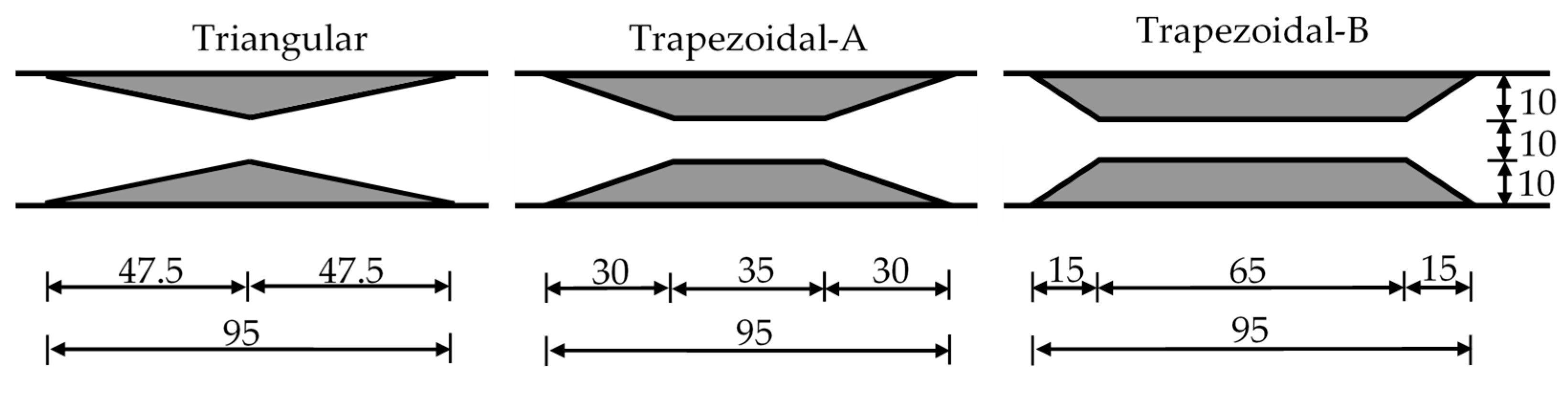
The dam-break flow originates right after the gate lifting, when it starts rapidly propagating on the dry channel, recorded all along the channel through the transparent glass walls by the three synchronous CCD cameras. Once the wave reaches the contracted section, the wave is partially reflected, thus inducing the formation of a negative bore moving upward, while the rest of the flow moves downward. 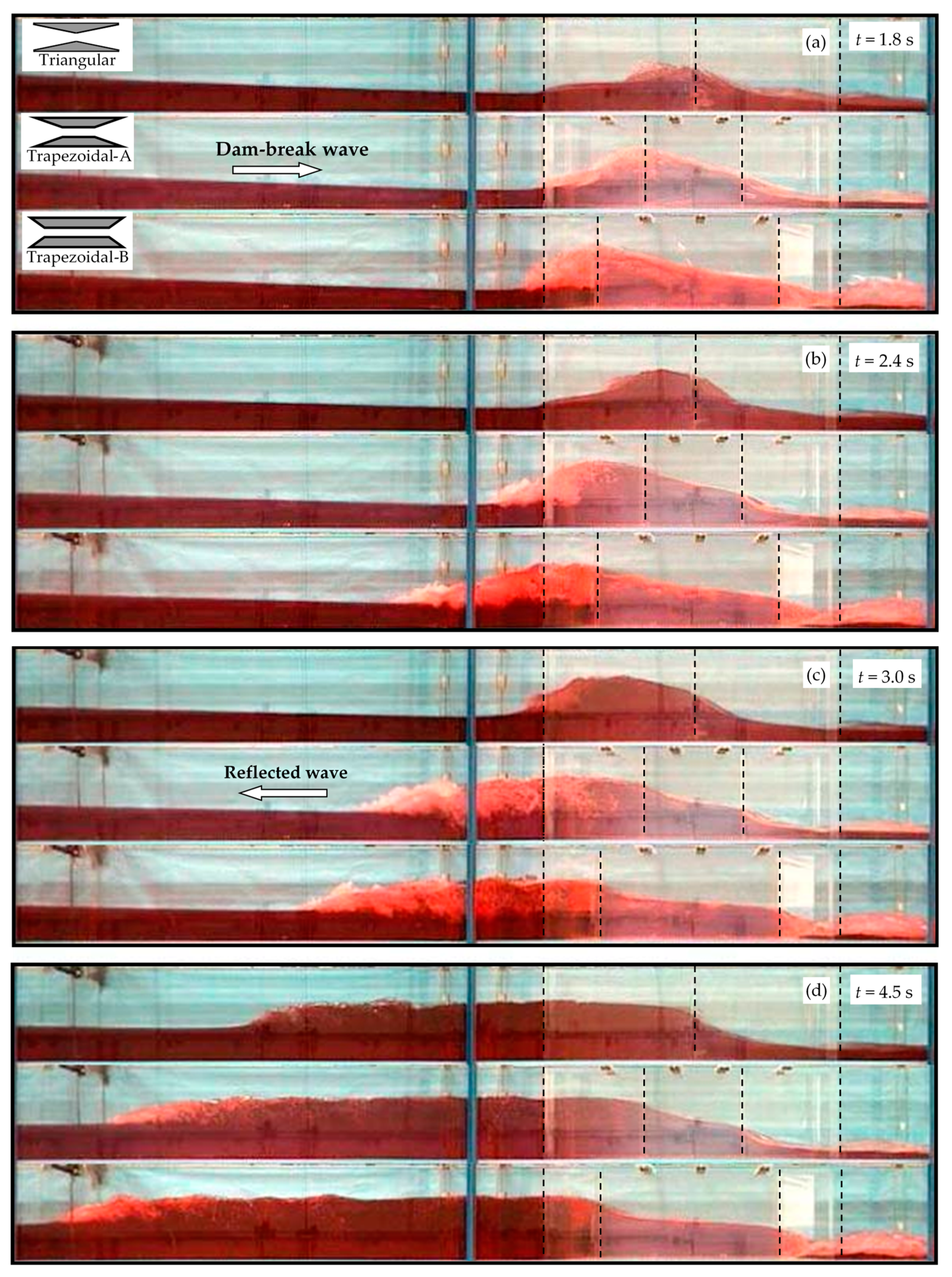In Figure 3, images obtained from the experiments conducted for the three different contractions, respectively, at different times after the gate opening are compared. The dashed lines indicate the borders of the contraction zone for all three cases. The blue line in the pictures is the supporting strut for the glass channel walls.

As shown in the images at t = 1.8 s (Figure 3a), the water level starts to rise at the points where the flood wave encounters the narrowest section, being it constricted by the local contraction; intense turbulence mixing is evident on the free surface, with strong air entrainment into the flow, and a negative bore of water-air swelling starts to move upward with rising depth. In the case of Trapezoidal-B contraction, for which the minimum section is reached earlier than with the other contractions, the water level rises faster. In addition, as a result of the flow sudden expansion downstream of the contraction, a significant formation of air bubbles is detected, differently from the other cases. On the other side, for the Triangular contraction, the rise in the water level is slower, being the narrowest section reached at a bigger distance, and a very small amount of air bubbles forms. At t = 2.4 s (Figure 3b), the negative wave is moving upward with rising water depth. In the case of Trapezoidal-B contraction, the surge wave moves upward with significant air entrainment in front of the wave. For the Triangular case, the water surface slope continues to increase in the narrowing section and there is almost no air entrainment. For the Trapezoidal-A contraction, the water surface has a bumpy shape with a maximum water level in the middle of the narrowing section, and significant air entrainment occurs in front of the reflected wave. At t = 3.0 s (Figure 3c), the water surface has a bumpy appearance at the narrowing section for the Triangular contraction, but there is still no significant air entrainment at the upfront wave surface. The reflected wave in the Trapezoidal-B case moves little ahead and strong air entrainment is observed compared to Trapezoidal-A. These reflection waves can be considered a moving hydraulic jump. At t = 4.5 s (Figure 3d), for the Triangular case, the reflected wave is still propagating, with still little air entrainment in front of the wave compared to Trapezoidal-A and Trapezoidal-B; the reflected water wave moves slowly compared to the others. In all three cases, the water surface has a horizontal profile between the wave front and the first narrowed section, and the water level decreases rapidly after the contraction zone. In addition, the water surface slope in the narrowest region decreases from Triangular to Trapezoidal-B contraction, i.e., with the slope of the contraction. As a result, in the case of Trapezoidal-B, it can be said that stronger reflections occur with the passage of the flood wave, there is significant air entrainment in front of the surge wave, and the wave front moves faster upward, compared to Trapezoidal-A and even more compared to Triangular contractions. The reason for this behavior can be ascribed to the fact that in the Trapezoidal-B case, the flow cross-section has a more rigid transition due to the higher slope of the contracting obstacles and the shorter tapered upstream section, resulting in an earlier encounter with the narrowest opening, compared to the other cases. On the other hand, in the Triangular contraction case, the transition from the full cross-section to the narrowest section is smoother, the flow is more slowly constricted at the local contraction entrance, the wave front jams and runs up the channel sidewalls with less impact, and the water reflection remains smaller.

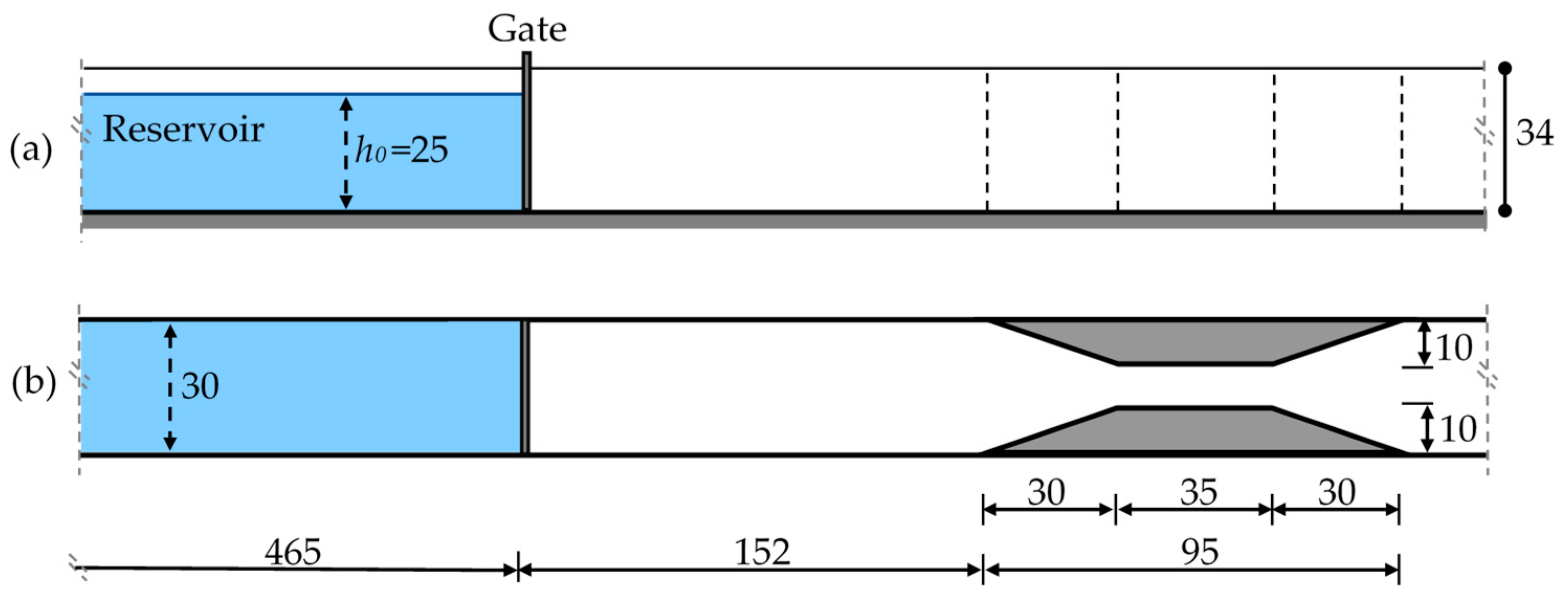
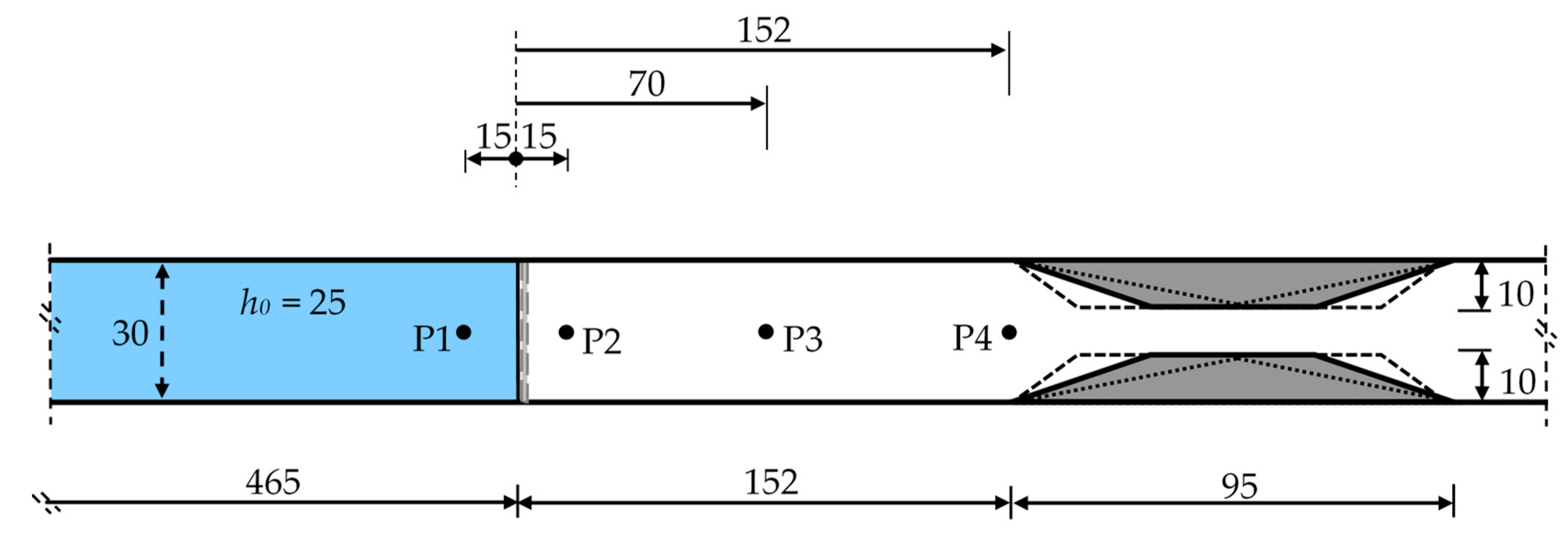
Besides the water surface profiles at different times, time variation of water levels was also measured at four different points in the three cases using the virtual wave probe. The measurement points (Figure 4) were selected, respectively as follows: right upstream of the dam (P1), right downstream of the dam (P2), at half distance between the dam location and the contraction (P3), and at the starting point of the contraction (P4).

Figure 5 displays a comparison of the time variation of the water level for all the contraction cases in non-dimensional form: the initial water depth h₀ was used as denominator of horizontal distance (X = x/h₀) and flow depth (h/h₀), whereas time t was multiplied by (g/h₀)^1/2, with g gravity acceleration, to get the non-dimensional form of time T = t (g/h₀)^1/2.

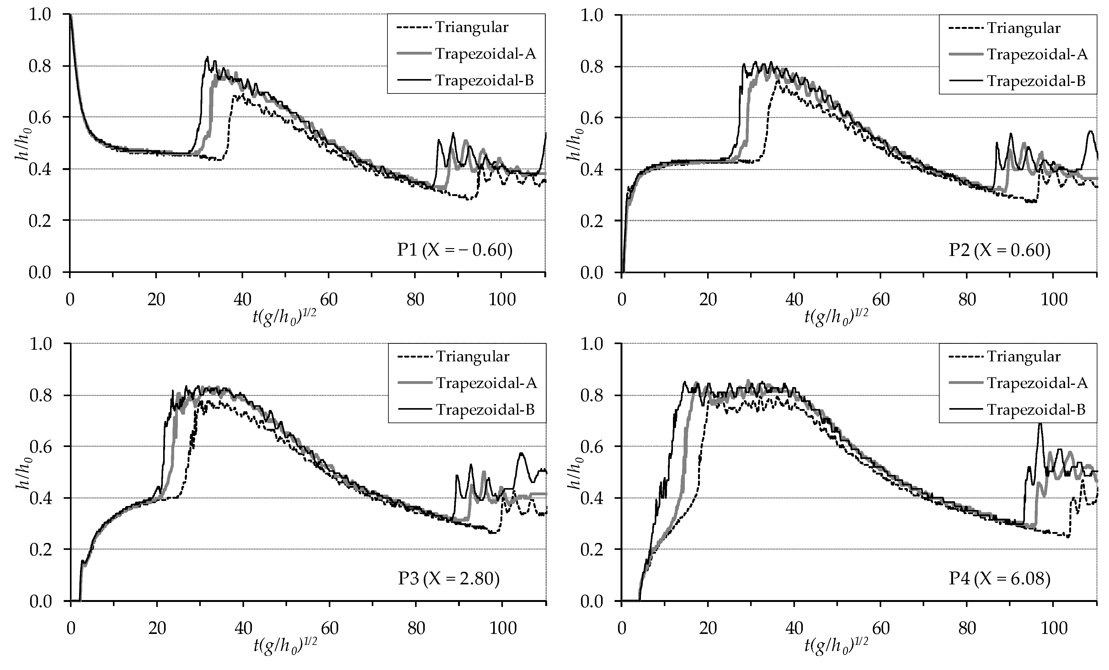
Since the initial water level in the reservoir is the same ($h_0$ = 0.25 m), with the opening of the vertical gate simulating the dam-break, the rapid decrease in water level at point P1 and the rapid increase in water level at points P2 and P3 at initial stages coincide for all three cases. At point P4 where the contraction begins, the differences between the water levels are remarkable, since the time between the arrival of the flood wave and the formation of the reflected wave is very short. Since the distance between the measurement point P4 and the narrowest section is very short for Trapezoidal-B, the water level rises continuously and rapidly with the flood wave reaching and reflecting, whereas for the Triangular contraction, the narrowing distance is little longer and the difference in the rise of water due to the incoming and reflected waves is more pronounced. In addition, at point P4, the non-dimensional time T to reach the maximum height of water level is 10.52 for the Trapezoidal-B, 13.53 for the Trapezoidal-A and 16.91 for the Triangular case, respectively, i.e., in the Triangular contraction is longer than in the other cases. The maximum water levels were observed at the narrowest section for all cases. The measured non-dimensional maximum water height h/h₀ is 0.85 for Trapezoidal-B, 0.84 for Trapezoidal-A and 0.81 for Triangular contraction, i.e., it is higher, since it is reached with more abrupt contraction, in the Trapezoidal-B case. Similar results are obtained observing the graphs of P1, P2 and P3 points. With the Trapezoidal-B contraction, the reflected wave reaches these points earlier and the measured maximum height is higher compared to the other cases; the water level in the upstream sections of the contraction increases significantly with the formation of a negative surge (reflected) wave in all cases. Due to finite reservoir length, the flow rate of the incoming flow decreases after a while and the water accumulated upstream of the contraction also gradually decreases. The reflected wave moving upwards is again reflected from the vertical wall at the upstream end of the channel, and a wave train which moves again downstream is formed. In the plots, while water levels are decreasing, a sudden rise and fluctuation of water levels are observed. The comparison of the reflected waves for all cases shows that the wave reflected in the Trapezoidal-B case is faster than in the other cases. In addition, during the passage of the wave reflected from the upstream channel boundary through the contracted section, the water level increases considerably, especially for the Trapezoidal-B case (before T = 100). Then, the wave reflected from the upstream end of the channel is reflected again from the narrowed sections and starts to move again in the upstream direction. This situation can be seen in the Trapezoidal-B curve at T = 105 for points P2 and P3. In general, when the dam-break wave encounters a cross-sectional change during its propagation, while a part of the flow passes through the existing opening, the rest of it is reflected in the contracted section and forms a reflected wave moving upward between the contraction and the upstream end of the channel until the water completely discharges. As a result, when the dam-break flood wave encounters quite abrupt transitions along its path, stronger reflections, higher water levels and mixed flow conditions occur upstream of the narrowing section. The small oscillations observed in the experimental reconstruction of the water level time histories (Figure 5) with the specific image analysis measuring technique described above are not only the result of the strong reflections of propagating waves upward and downward and their interferences, but even more a result of the mixed flow conditions which occur in such strongly unsteady flows.

4.2. Comparison between Experimental and Numerical Results for Trapezoidal-A Case

Figure 6 displays, for the Trapezoidal-A case, the comparison between the numerical results obtained by CFD simulation of RANS (Figure 6a) and the experimental flow picture frames captured for the time interval 1.5–4.0 s (Figure 6b). The two frames at corresponding times are in good agreement.

The selected times from 1.5 s to 4.0 s permit one to analyze the formation and propagation of the negative bore. The dashed lines indicate borders of the local contraction and of the 0.65 m long narrow throat. As already seen in Figure 3 for all cases, with the sudden opening of the gate, the flow starts propagating; when the traveling wave front reaches the local contraction, at first the flow cross-section is constricted at the entrance before jamming and running up the sidewalls (t = 1.5 s). The water level sharply increases up to the entrance of the narrow throat at times t = 1.5–1.8 s, and intense turbulence mixing, with air entrainment into the flow, is noticed on the free surface. At time t = 2.1 s, the negative bore crest starts moving upstream with rising depth. When the bore crest leaves the contraction region (t = 2.4 s), a reflected negative wave moving upwards forms (t = 2.7 s). In this way, the flood wave moving downwards encounters the negative wave, thus forming a prominent hydraulic jump at the contraction entrance.

The rapid rise in water level right upstream of the contraction entrance and the formation of the negative bore can be justified by the relationship between instantaneous specific energy and minimum energy of the propagating wave. The specific energy of the flow is smaller than the minimum energy necessary to pass through the contraction. Considering an upstream supercritical flow, a channel contraction induces an increase in flow depth to gain potential energy. Then, the flow transcends abruptly to subcritical with consequent formation of a hydraulic jump and a negative wave. 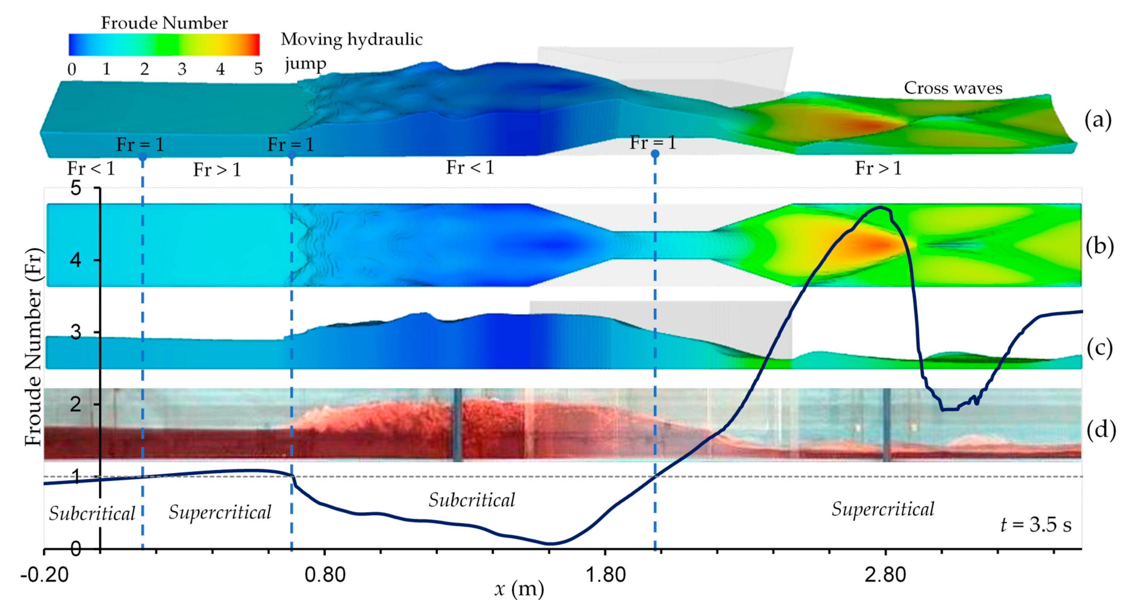This hydraulic jump moves upward as a rolling negative bore due to transient flow conditions [50]. In the narrowest section, the water depth decreases rapidly and the flow passes through the critical depth. Once passed over the narrowest section, the flow becomes supercritical and cross waves form downstream due to the new expansion of the cross section along the final part of the obstacle. This analysis is also well represented in Figure 7, in which at a given time (t = 3.5 s) the variation of Froude number (Fr) values along the channel is superimposed on the numerical solution (given as 3D view in Figure 7a, plan view in Figure 7b, and front view in Figure 7c) and on the experimental captured image as water longitudinal profile (in Figure 7d). The values of Fr number in the plot are those at the centerline of the cross section along the channel. As shown in the figure, critical regimes (Fr = 1) can be observed at three different sections: at x = 0.18 m (just downstream of the dam), x = 0.69 m (near half-distance of the throat) and x = 1.98 m (at reflected wavefront with moving hydraulic jump), respectively, having regimes from subcritical (Fr < 1) to supercritical (Fr > 1) and vice-versa. Minimum Fr number was observed right after the flow enters the throat (at x=1.60 m as Fr = 0.067). Maximum Fr number was observed downstream of expansion (x = 2.78 m as Fr = 4.72), coinciding with the location where the cross wave first occurs. At the location where the cross wave intersects (x = 3.00 m as Fr = 1.92), Fr number value decreases, still staying in supercritical flow regime. However, as the flow accelerates, Fr number increases again due to cross wave. It can be said that when the flood wave encounters a contraction while propagating downstream, flow regimes rapidly change from supercritical to subcritical and vice versa due to obstacle and mixed flow conditions occurring along the channel. Modeling of the mixed flow regimes requires special attention due to the different directions of wave propagation in subcritical and supercritical flows, as they contain shocks [23]. Similar mixed flow conditions are observed when the dam-break wave encounters a bottom obstacle [27].

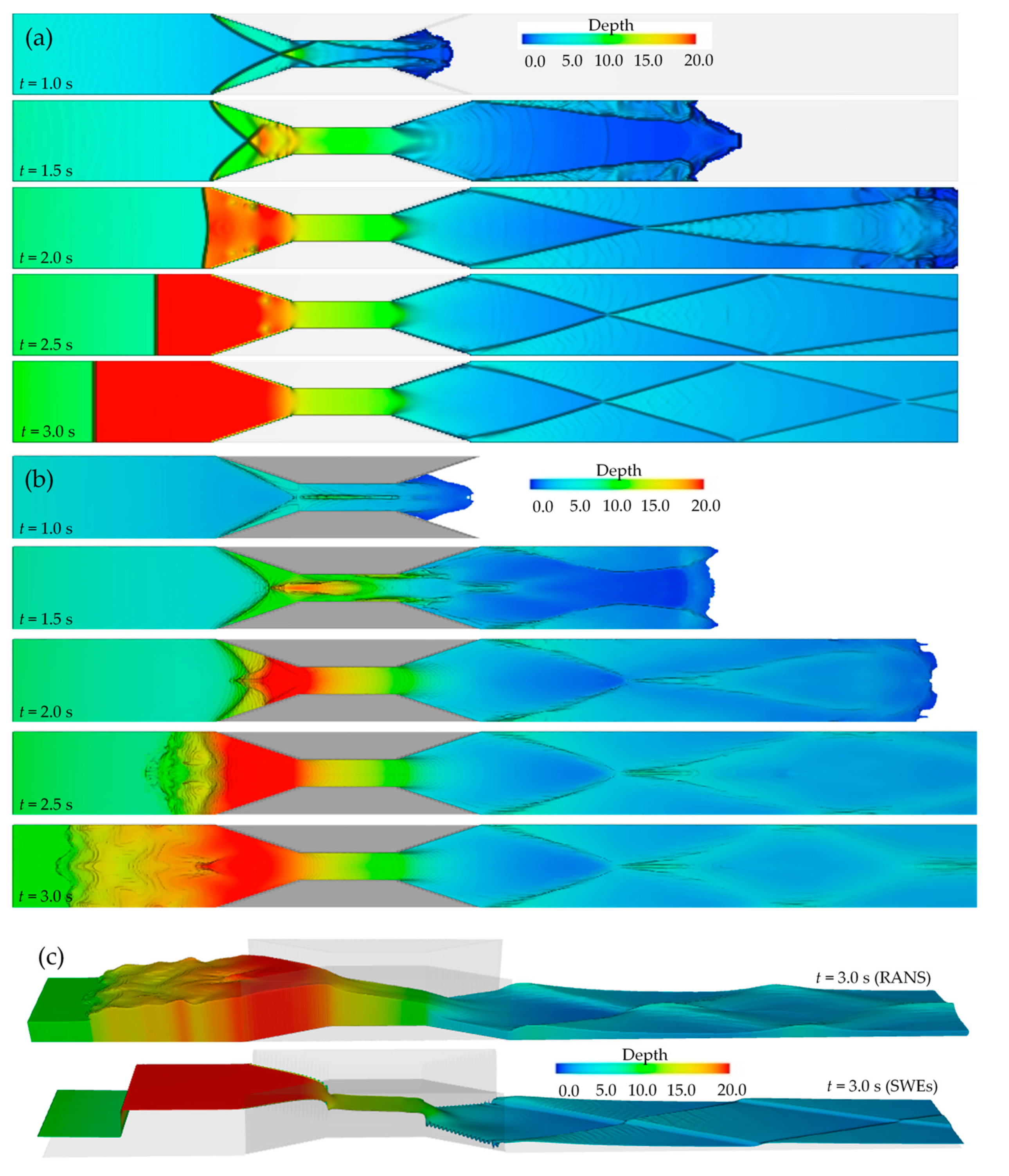
Figure 8 shows flow depths along the contracting and expanding part of the channel at initial stages of the dam-break flow obtained from SWEs and RANS approaches of FLOW-3D, respectively. The direction of the unsteady flow is from left to right; the view is from the top of the channel in Figure 8a,b, whereas Figure 8c displays a 3D view.

The formation of negative waves due to the channel contraction, and their propagation upward are clearly observed for both models. Moreover, because of the expansion in the terminal part of the obstacles, cross waves appear downstream of the contraction [42]. After t = 2.5 s, the sharp border between the two colors (blue and red) in Figure 8a represents the discontinuity at the negative wave front in the SWEs solution, which is also observed in the 3D view in Figure 8c for t = 3.0 s. Figure 8b evidently mirrors the formation of the hydraulic jump produced by the channel contraction and the occurrence of supercritical flows after the narrow throat.

Whenever a supercritical flow encounters any obstacle, such as expansion or contraction, a surface wave moving across the flow forms. The contraction forces the flow to pass through the critical depth; thus, oblique jumps arise at the end of the contraction where the diffraction angles start, and they are carried downward as cross waves. Interferences between waves result in a disturbance pattern of cross waves, which can be qualitatively observed in Figure 8. Wave fronts generated by the oblique jumps on both walls bounce back and forth between the side walls, with subsequent formation of an oblique jump moving toward the centerline and, the flow pattern being symmetric, generating a backward wave front toward the wall, as if there is a solid wall in the centerline. These continuous oblique jumps produce turbulent disturbances in the water surface [42].

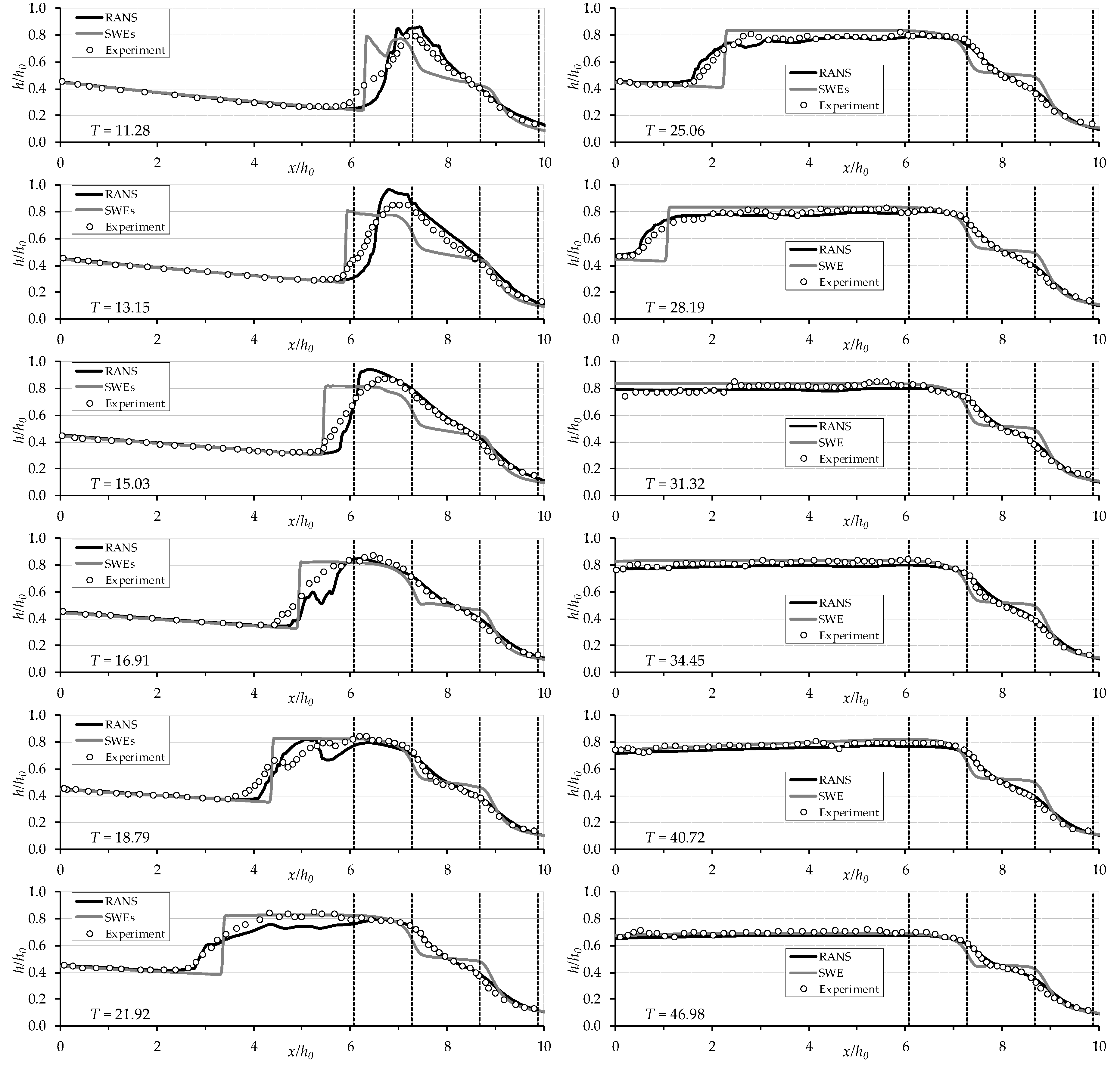
Figure 9 shows the comparison between the computed and the measured free surface profiles at various times after the gate removal in the Trapezoidal-A contraction case.

The borders of the contraction region are X = 6.08 and X = 9.88, indicated with dashed lines on the graphs, together with the borders of the throat. Again, it can be noticed that when the propagating dam-break wave approaches the contraction (T = 11.28), the water level upstream rises abruptly and a negative wave is formed. A satisfactory accordance between measured and both computed profiles can be observed at X < 5 at times T = 11.28–15.03. A little discrepancy is noticed between experimental and RANS solved numerical free-surface profiles between X = 6 and about X = 9, whereas the SWEs solution shows more discrepancies and underestimates water depths as well as the negative wave front speed. The formation of the strong hydraulic jump causes here random oscillations. Free surface profiles can be nearly predicted by both numerical simulations after T = 18.79, except for the appearance of a discontinuity on the negative wave front in the SWEs solutions. The overall disagreement of the SWEs solution is most probably caused by the assumption of neglectable vertical acceleration and hydrostatic pressure distribution [2].

When the formation of the negative wave is fully completed (i.e., at times T ≥ 21.92), the free surface becomes more stable and a better correspondence is observed between the measured profiles and those computed by RANS. While the RANS model slightly underestimates the maximum water levels for T ≥ 21.92, the SWEs solution overestimates them.

The present investigation analyzes the capability of the two models to simulate dam-break flows in real-case topography. It is shown that the solution of the VOF-based RANS numerical model well describes well the propagation of the negative wave induced by the strong reflection of the dam-break flow against the abruptly changing topography with a reasonable accuracy, but it needs more computational time. On the other hand, the SWEs simulation shows a little disagreement but it provides an advantage in requiring less computational time, which would be even more important for real-case real-scale applications. The run-times were approximately 53 min in SWEs and 46 h in RANS for 20 s solution time, respectively, on a computer equipped with Intel Core i7 2.8 GHz 16 GB RAM. Hence, SWE-based numerical models are still preferable over RANS-based models for large computational domains where the vertical acceleration is insignificant compared to the less computational efforts and time. Fine meshes can be necessary in numerical simulations to represent irregular topographies and to obtain more accurate results. On the other hand, more computational efforts and times are required for 3-D solutions of large-scale real-case dam-break problems in the presence of artificial and natural obstacles such as bridges, buildings, dikes, and trees [39,51,52]. In order to model flow around 3D structures such as bridges using fine mesh to capture localized flow details, the hybrid models combining RANS-based 3D flow and shallow water models in one simulation can also be used to reduce the computation time [44].

Figure 10 shows the location of eight measurement points (P1–P8) for a further analysis, in which time histories of water levels using virtual wave probes were obtained and compared with SWEs and RANS results for the Trapezoidal-A case.

Figure 11 shows the comparison between numerical (RANS and SWEs) and experimental results in terms of non-dimensional water level changes with time at all measurement points (P1 to P8) for the Trapezoidal-A case.

Once the gate representing the dam is instantaneously lifted, a sudden drop for P1 and rise for P2 in water levels are observed up to T = 5, with the two measuring points located just upstream and downstream of the dam, respectively. In these sections, a very little variation in water levels is observed between T = 5–30. At point P3 (X = 2.80), the rise in the water level is slower as the dam-break flood wave passes until T = 20. Until the wave reflected from the contraction reaches the measurement points, at T = 30 for P1 and P2 and at T = 20 for P3, a good correspondence is observed between experimental and numerical results both for the RANS and the SWEs solutions. Only the SWEs profile is slightly lower during the decrease of the water level in the reservoir at P1. When the reflected wave reaches the measuring points, the water level increases suddenly at this point. If the RANS-calculated maximum water levels are in good accordance with the experiments, the results are overestimated by the SWEs. At the entrance of the contraction (at X = 6.08 for P4 and at X = 6.68 for P5), an abrupt rising in water level, due to the very short time between the arrival of the flood wave and the formation of the reflected wave, is accurately simulated in the RANS solution except for the peak level at P5. Similarly, due to the absence of any reflection, a continuous rapid rise in water level was observed at P6, P7 and P8 points. Water-level changes were also accurately predicted by the SWEs, except for when the reflected wave forms and propagating wave passes through the contraction, because of neglecting the vertical acceleration and assuming hydrostatic pressure distribution in the SWEs approach. Therefore, the water levels having more water surface curvature at both ends of the throat at points P6 (X = 7.28) and P8 (X = 8.68) were significantly underestimated and overestimated, respectively. A similar situation can also be clearly seen at the beginning and end of the narrowest section in Figure 9 for times T = 16.91–46.98. When the reflected wave moving upward reaches the dam axis, the water level gradually drops due to the finite reservoir length. The flow transcends to subcritical at the downstream of the reflected wave front due to the hydraulic jump and flows freely through the opening of the contraction. At this stage, the correspondence between experimental and both computational results are quite satisfactory. Unlike the numerical simulations, in the experiments, minor fluctuations occur on the water surface in all graphs at the stages in which the maximum water levels occur and water level decreases. This situation is due to the moving hydraulic jump caused by the flow transition from supercritical to subcritical at the wave front after reflection of the dam-break wave from the contraction. Some undulations also emerge from the difficulty in determining the free-surface edge in experiments due to the foaming in proximity to the wave front [15,21]. The computed water levels, wave front velocities and amplitude of the wave train formed by the reflection of the negative wave against the upstream end wall are also in good agreement with experimental results. However, the speed of the wave train is slightly faster for all measurement points in experiments than the SWEs but lower than the RANS.

The RANS model uses the sum of viscous and turbulent shear stresses with turbulence models, whereas the SWEs use an empirical equation to calculate bottom shear stress for turbulent flows. Therefore, when comparing RANS and SWEs results in terms of water-level measurements, it should be taken into consideration that energy losses between the two models are handled with different approaches. The SWEs in FLOW-3D do not include any viscosity term nor use any of the turbulent models, but rely on the empirical expression based on a quadratic law given in Equation (10) to calculate energy loss for turbulent flow. The calculation of bottom shear stress requires the definition of a drag coefficient $C_D$, which can be selected as a constant (as we did, assigning the value of 0.0026, according to the manual suggestions) or let it be calculated from the software for a component, based on its surface roughness, using Equation (11). Preliminary sensitivity studies showed that the use of a constant value $C_D$ = 0.0026 or of a value of $C_D$ calculated based on the surface roughness ks = 0.00015 cm did not change much the results in terms of water depths. A sensitivity analysis of the calibration parameter, evaluating the effect of different $C_D$ values, was also performed, proving no significant effects in maximum wave heights and speed of reflected wave fronts. This is probably due to the low roughness of bottom and walls of the channel, which were made of glass. An accurate determination of the $C_D$ coefficient might be necessary for surfaces with different roughness.

The dam-break wave propagation analyzed here is a strongly unsteady flow characterized by high turbulence, mixed flow and steep water surface fronts (shocks). In this situation, the hypotheses of hydrostatic distribution of pressures and neglectable vertical components of both velocity and acceleration, on which the SWEs are based, are not satisfied and can lead to not completely satisfactory results, differently from a fully 3D model like RANS, which is certainly more suitable. However, during the transition of the wave, water levels are excessive only in a certain period of time in the SWEs results. In the 3D RANS model energy losses are fully calculated via shear stress expressions with viscosity and turbulent viscosity by using k-ε turbulent model. For a more coherent comparison between SWEs and RANS, which is not a priority here, it might be better to evaluate at each time step water levels also in the SWEs model, including the period of time in which the hydraulic jump (shock) occurs.

Error analysis was performed making use of the three following measures of the differences between model (RANS and SWEs) predicted $y_p$ and experimental observed values $y_0$ for n samples:

• Root Mean Square Error (RMSE)

  $$\mathrm{RMSE}=\sqrt{\frac{1}{\mathrm{n}}{\displaystyle \sum }_{i=1}^{\mathrm{n}}{\left(y_{\mathrm{o}}-y_p\right)}^2}$$

  (17)
• Mean Absolute Percent Error (MAPE)

  $$\mathrm{MAPE}\%=\frac{100}{\mathrm{n}}\times {\displaystyle \sum }_{i=1}^{\mathrm{n}}\left|\frac{y_{\mathrm{o}}-y_p}{y_0}\right|$$

  (18)
• Mean Absolute Error (MAE)

  $$\mathrm{MAE}=\frac{1}{\mathrm{n}}{\displaystyle \sum }_{\mathrm{i}=1}^{\mathrm{n}}\left|y_{\mathrm{o}}-y_p\right|$$

  (19)

Referring, for example, to the data reported in Figure 11 (water level time histories), the three errors are reported for the measuring points P1–P8 in

Table 2. Error analysis referred to the comparison between numerical (RANS and SWEs, respectively) and experimental results for water-level time histories at measurement points P1–P8.

Errors	RANS
	P1	P2	P3	P4	P5	P6	P7	P8
MAPE %	3.50	4.10	4.38	5.57	5.34	7.16	7.67	7.50
RMSE (cm)	0.82	0.79	0.80	0.80	0.96	1.45	1.20	0.65
MAE (cm)	0.42	0.45	0.53	0.63	0.56	0.73	0.53	0.46
Errors	SWEs
	P1	P2	P3	P4	P5	P6	P7	P8
MAPE %	4.22	4.37	4.82	7.90	7.26	18.14	5.88	13.80
RMSE (cm)	0.98	0.84	0.88	1.71	1.50	2.39	0.85	1.42
MAE (cm)	0.54	0.51	0.56	0.86	0.78	2.02	0.51	1.09

. Errors were calculated for 900 (18/0.02) different values for a total of 18 s at 0.02 s intervals.

In general, the error rates in SWE were higher than RANS for all of the methods. As mentioned above and observed in Figure 11, the absolute highest error rate for SWE was observed at the entrance and exit of the contraction zone (P6 and P8), equal to 18.14% and 13.80%, respectively (MAPE calculation). In the same contraction zone, the highest error was also obtained for RANS (7.67 with MAPE calculation). The lowest errors were reached for the more upstream measurement points, as 4.22% for SWEs and 3.50% for RANS. In addition, similar results were observed for RMSE and MAE, especially with respect to the highest error at P6 for RANS and SWEs.

As a result, for all sections, both RANS’s and SWEs’ numerical simulations were able to successfully reproduce variation of the water levels over time. However, the peak water levels on the reflected wave crest are overestimated in the SWEs results. Reflected wave propagation velocity is slightly faster in the RANS than in both experiments and SWEs simulations. The flow is truly 3D, with significant air entrainment, which cannot be entirely captured by the 2D SWEs numerical model. Better results can be obtained by RANS with turbulence closures, but requiring more computational effort for the 3D dam-break flow, whereas the SWEs-based numerical models need less computing power and shorter computational time in large-scale problems with reasonable accuracy. If the flow, in fact, is truly 3D just upstream of the contraction, then it can be assumed to be 2D except at the converging part of the obstacle and for the initial stage of the dam break; therefore the SWE approach can be accepted overall for the reasonable prediction of the dam-break flow [31,53,54].

5. Conclusions

The dam-break wave propagation in a channel with three different lateral contraction geometries (one triangular and two trapezoidal with different slopes) was investigated experimentally and numerically.

A digital image analysis technique was used for flow measurement, providing useful laboratory data without any interference of physical devices with the flow. The flow propagation through the transparent channel walls was recorded, and then continuous free surface profiles and time histories of water levels were obtained through synchronous and non-intrusive acquisition by virtual wave probe. The experimental evidence shows that the abrupt sidewall contraction in the channel cross-section produces a partial reflection of the wave against the contraction itself and the formation of a negative bore, which propagates upstream, while the rest of the flow keeps travelling downstream. This reflected wave (negative wave) can also be considered as a moving hydraulic jump. In the upstream zone of the contraction region, when the dam-break flood wave encounters obstacles having geometrically different abrupt transitions along its path, stronger reflections, higher water levels and unsteady mixed flow conditions were observed more clearly for sharp than for smooth contractions (from Trapezoidal-B to Triangular).

The laboratory data were compared against the SWEs and 3D RANS (with the k-ε turbulence closure model) numerical simulation results, obtained through a VOF-based commercially available CFD program, FLOW-3D. There is a very satisfactory accordance between measured data and RANS numerical results, while the SWEs solution shows little discrepancies at early stages of the reflected wave formation. Despite inaccurate prediction of the negative bore formation and overestimation of the peak water levels, the SWEs model is still capable of predicting the free surface profiles with an acceptable level. Although the RANS based numerical models with turbulence closures give better results for 3-D dam-break flow over the irregular domains, the SWEs-based numerical models need less computing power and give faster results in large scale problems with reasonable accuracy.

Owing to the fact that limited field data available for dam-break flows, the present new experimental data give a contribution to the understanding of the effect of a dam-break wave propagation over an abruptly varying downstream topography. Although the laboratory investigated scenarios (e.g., the rectangular channel) are often far from reality (e.g., a real river bed), in fact, results obtained from small-scales tests conducted in a protected and controlled environment can be useful for a deeper comprehension of the real processes and for the validation of simulation numerical models, also in large-scale scenarios for real-time defense systems. Results confirm that simplified SWEs-based models can be used for analyzing a large number of scenarios, but they have to be integrated with more complete RANS simulations for more accurate results.

References

1. de Marinis, G.; Di Cristo, C.; Evangelista, S.; Leopardi, A. Dam break waves on stepped bottom. In Proceedings of the XXXIII IAHR Int. Biennal Congress, Vancouver, BC, Canada, 8–14 August 2009; pp. 1262–1268. [Google Scholar]
2. Evangelista, S.; Altinakar, M.S.; Di Cristo, C.; Leopardi, A. Simulation of dam-break waves on movable beds using a multi-stage centered scheme. Int. J. Sediment Res. 2013, 28, 269–284. [Google Scholar] [CrossRef]
3. Ozmen-Cagatay, H.; Kocaman, S.; Guzel, H. Investigation of dam-break flood waves in a dry channel with a hump. HydroResearch 2014, 8, 304–315. [Google Scholar] [CrossRef]
4. Wang, B.; Zhang, J.; Chen, Y.; Peng, Y.; Liu, X.; Liu, W. Comparison of measured dam-break flood waves in triangular and rectangular channels. J. Hydrol. 2019, 575, 690–703. [Google Scholar] [CrossRef]
5. Valiani, A.; Caleffi, V.; Zanni, A. Case Study: Malpasset Dam-break simulation using a two-dimensional finite volume method. J. Hydraul. Eng. 2002, 128, 460–472. [Google Scholar] [CrossRef]
6. Gallegos, H.A.; Schubert, J.E.; Sanders, B.F. Two-dimensional, high-resolution modeling of urban dam-break flooding: A case study of Baldwin Hills, California. Adv. Water Resour. 2009, 32, 1323–1335. [Google Scholar] [CrossRef]
7. Prestininzi, P. Suitability of the diffusive model for dam break simulation: Application to a CADAM experiment. J. Hydrol. 2008, 361, 172–185. [Google Scholar] [CrossRef]
8. Haltas, I.; Tayfur, G.; Elçi, Ş. Sebnem Two-dimensional numerical modeling of flood wave propagation in an urban area due to Ürkmez dam-break, İzmir, Turkey. Nat. Hazards 2016, 81, 2103–2119. [Google Scholar] [CrossRef] [Green Version]
9. Güney, M.S.; Tayfur, G.; Bombar, G.; Elçi, Ş. Distorted physical model to study sudden partial dam break flows in an urban area. J. Hydraul. Eng. 2014, 140, 05014006. [Google Scholar] [CrossRef] [Green Version]
10. Miller, S.; Chaudhry, M.H. Dam-break flows in curved channel. J. Hydraul. Eng. 1989, 115, 1465–1478. [Google Scholar] [CrossRef]
11. Bell, S.W.; Elliot, R.C.; Chaudhry, M.H. Experimental results of two-dimensional dam-break flows. J. Hydraul. Res. 1992, 30, 225–252. [Google Scholar] [CrossRef]
12. Ostapenko, V.V. Dam-break flows over a bottom step. J. Appl. Mech. Tech. Phys. 2003, 44, 495–505. [Google Scholar] [CrossRef]
13. Soares-Frazao, S. Experiments of dam-break wave over a triangular bottom sill. J. Hydraul. Res. 2007, 45, 19–26. [Google Scholar] [CrossRef]
14. Soares-Frazao, S.; Zech, Y. Experimental study of dam-break flow against an isolated obstacle. J. Hydraul. Res. 2007, 45, 27–36. [Google Scholar] [CrossRef]
15. Ozmen-Cagatay, H.; Kocaman, S. Investigation of dam-break flow over abruptly contracting channel with trapezoidal-shaped lateral obstacles. J. Fluids Eng. 2012, 134, 081204. [Google Scholar] [CrossRef]
16. Bellos, C.V.; Soulis, V.; Sakkas, J.G. Experimental investigation of two-dimensional dam-break induced flows. J. Hydraul. Res. 1992, 30, 47–63. [Google Scholar] [CrossRef]
17. Cochard, S.; Ancey, C. Tracking the free surface of time-dependent flows: Image processing for the dam-break problem. Exp. Fluids 2007, 44, 59–71. [Google Scholar] [CrossRef]
18. Aureli, F.; Maranzoni, A.; Mignosa, P.; Ziveri, C. Dam-break flows: Acquisition of experimental data through an imaging technique and 2D numerical modeling. J. Hydraul. Eng. 2008, 134, 1089–1101. [Google Scholar] [CrossRef]
19. Aureli, F.; Maranzoni, A.; Mignosa, P.; Ziveri, C. An image processing technique for measuring free surface of dam-break flows. Exp. Fluids 2010, 50, 665–675. [Google Scholar] [CrossRef]
20. Liu, W.; Wang, B.; Chen, Y.; Wu, C.; Liu, X. Assessing the analytical solution of one-dimensional gravity wave model equations using dam-break experimental measurements. Water 2018, 10, 1261. [Google Scholar] [CrossRef] [Green Version]
21. Kocaman, S.; Ozmen-Cagatay, H. Investigation of dam-break induced shock waves impact on a vertical wall. J. Hydrol. 2015, 525, 1–12. [Google Scholar] [CrossRef]
22. Wang, B.; Liu, W.; Wang, W.; Zhang, J.; Chen, Y.; Peng, Y.; Liu, X.; Yang, S. Experimental and numerical investigations of similarity for dam-break flows on wet bed. J. Hydrol. 2020, 583, 124598. [Google Scholar] [CrossRef]
23. Mohapatra, P.; Bhallamudi, S.M. Computation of a dam-break flood wave in channel transitions. Adv. Water Resour. 1996, 19, 181–187. [Google Scholar] [CrossRef]
24. García-Navarro, P.; Fras, A.; Villanueva, I. Dam-break flow simulation: Some results for one-dimensional models of real cases. J. Hydrol. 1999, 216, 227–247. [Google Scholar] [CrossRef]
25. Brufau, P.; Vázquez-Cendón, M.E.; García-Navarro, P. A numerical model for the flooding and drying of irregular domains. Int. J. Numer. Methods Fluids 2002, 39, 247–275. [Google Scholar] [CrossRef]
26. Gottardi, G.; Venutelli, M. Central scheme for two-dimensional dam-break flow simulation. Adv. Water Resour. 2004, 27, 259–268. [Google Scholar] [CrossRef]
27. Ozmen-Cagatay, H.; Kocaman, S. Dam-break flow in the presence of obstacle: Experiment and CFD simulation. Eng. Appl. Comput. Fluid Mech. 2011, 5, 541–552. [Google Scholar] [CrossRef] [Green Version]
28. Marsooli, R.; Wu, W. Three-dimensional numerical modeling of dam-break flows with sediment transport over movable beds. J. Hydraul. Eng. 2015, 141, 04014066. [Google Scholar] [CrossRef]
29. Liang, D.; Falconer, R.; Lin, B. Comparison between TVD-MacCormack and ADI-type solvers of the shallow water equations. Adv. Water Resour. 2006, 29, 1833–1845. [Google Scholar] [CrossRef]
30. Liang, Q.; Marche, F. Numerical resolution of well-balanced shallow water equations with complex source terms. Adv. Water Resour. 2009, 32, 873–884. [Google Scholar] [CrossRef]
31. Evangelista, S. Experiments and numerical simulations of dike erosion due to a wave impact. Water 2015, 7, 5831–5848. [Google Scholar] [CrossRef] [Green Version]
32. Erduran, K.S.; Kutija, V.; Hewett, C.J.M. Performance of finite volume solutions to the shallow water equations with shock-capturing schemes. Int. J. Numer. Methods Fluids 2002, 40, 1237–1273. [Google Scholar] [CrossRef]
33. Shigematsu, T.; Liu, P.; Oda, K. Numerical modeling of the initial stages of dam-break waves. J. Hydraul. Res. 2004, 2, 183–195. [Google Scholar] [CrossRef]
34. Biscarini, C.; Di Francesco, S.; Ridolfi, E.; Manciola, P. On the simulation of floods in a narrow bending valley: The malpasset dam break case study. Water 2016, 8, 545. [Google Scholar] [CrossRef] [Green Version]
35. Vasquez, J.A.; Roncal, J.J. Testing River2D and Flow-3D for sudden dam-break flow simulations. In Proceedings of the C.D.A. Annual Conference, Whistler, BC, Canada, 3–8 October 2009; pp. 44–55. [Google Scholar]
36. Biscarini, C.; Di Francesco, S.; Manciola, P. CFD modelling approach for dam break flow studies. Hydrol. Earth Syst. Sci. 2010, 14, 705–718. [Google Scholar] [CrossRef] [Green Version]
37. Ozmen-Cagatay, H.; Kocaman, S. Dam-break flows during initial stage using SWE and RANS approaches. J. Hydraul. Res. 2010, 48, 603–611. [Google Scholar] [CrossRef]
38. Marsooli, R.; Wu, W. 3-D finite-volume model of dam-break flow over uneven beds based on VOF method. Adv. Water Resour. 2014, 70, 104–117. [Google Scholar] [CrossRef]
39. Quecedo, M.; Pastor, M.J.; Herreros, M.; Fernández-Merodo, J.A.; Zhang, Q. Comparison of two mathematical models for solving the dam break problem using the FEM method. Comput. Methods Appl. Mech. Eng. 2005, 194, 3984–4005. [Google Scholar] [CrossRef]
40. Ye, Z.; Zhao, X. Investigation of water-water interface in dam break flow with a wet bed. J. Hydrol. 2017, 548, 104–120. [Google Scholar] [CrossRef]
41. Liang, Q. Simulation of shallow flows in nonuniform open channels. J. Fluids Eng. 2008, 130, 011205. [Google Scholar] [CrossRef]
42. Kocaman, S.; Ozmen-Cagatay, H. The effect of lateral channel contraction on dam break flows: Laboratory experiment. J. Hydrol. 2012, 432, 145–153. [Google Scholar] [CrossRef]
43. Lauber, G.; Hager, W.H. Experiments to dambreak wave: Horizontal channel. J. Hydraul. Res. 1998, 36, 291–307. [Google Scholar] [CrossRef]
44. Flow Science Inc. Flow-3D Users Manual; Flow Science Inc.: Santa Fe, NM, USA, 2016. [Google Scholar]
45. Launder, B.E.; Spalding, D. The numerical computation of turbulent flows. Comput. Methods Appl. Mech. Eng. 1974, 3, 269–289. [Google Scholar] [CrossRef]
46. Hirt, C.; Nichols, B. Volume of fluid (VOF) method for the dynamics of free boundaries. J. Comput. Phys. 1981, 39, 201–225. [Google Scholar] [CrossRef]
47. Roache, P.J. Perspective: A method for uniform reporting of grid refinement studies. J. Fluids Eng. 1994, 116, 405–413. [Google Scholar] [CrossRef]
48. Roache, P.J. Verification and Validation in Computational Science and Engineering; Hermosa publishers: Socorro, NM, USA, 1998. [Google Scholar]
49. Celik, I.B.; Ghia, U.; Roache, P.J.; Freitas, C.J.; Coleman, H.; Raad, P.E.; Coleman, H.P. Procedure of estimation and reporting of uncertainty due to discretization in CFD applications. J. Fluids Eng. 2008, 130, 078001. [Google Scholar]
50. Chanson, H. Unsteady turbulence in tidal bores: Effects of bed roughness. J. Waterw. Port, Coastal, Ocean Eng. 2010, 136, 247–256. [Google Scholar] [CrossRef] [Green Version]
51. Zhang, S.-H.; Xia, Z.; Yuan, R.; Jiang, X. Parallel computation of a dam-break flow model using OpenMP on a multi-core computer. J. Hydrol. 2014, 512, 126–133. [Google Scholar] [CrossRef]
52. Peng, Y.; Diao, W.; Zhang, X.; Zhang, C.; Yang, S. Three-dimensional numerical method for simulating large-scale freewater surface by massive parallel computing on a GPU. Water 2019, 11, 2121. [Google Scholar] [CrossRef] [Green Version]
53. Evangelista, S.; Greco, M.; Iervolino, M.; Leopardi, A.; Vacca, A. A new algorithm for bank-failure mechanisms in 2D morphodynamic models with unstructured grids. Int. J. Sediment Res. 2015, 30, 382–391. [Google Scholar] [CrossRef]
54. Di Cristo, C.; Evangelista, S.; Greco, M.; Iervolino, M.; Leopardi, A.; Vacca, A. Dam-break waves over an erodible embankment: Experiments and simulations. J. Hydraul. Res. 2017, 56, 196–210. [Google Scholar] [CrossRef]
Figure 1. Laboratory set-up: (a) Longitudinal view A-A, (b) Top view, (lengths in (cm), Trapezoidal-A contraction).
Water 12 01124 g001
Figure 2. Geometries and dimensions (lengths in (cm)) of the different contractions chosen for the experiments.
Water 12 01124 g002
Figure 3. Comparison of test images for 3 different contraction conditions (dashed lines highlights the contraction position) in terms of water profiles at different times: (a) 1.8 s, (b) 2.4 s, (c) 3.0 s, (d) 4.5 s, respectively, after the gate opening.
Water 12 01124 g003
Figure 4. Measurement points for all cases: P1, P2, P3 and P4.
Water 12 01124 g004
Figure 5. Comparison of the time variation of water level for the three different contraction cases.
Water 12 01124 g005
Figure 6. Water profiles with formation and propagation of the negative bore for Trapezoidal-A case: (a) numerical solution (RANS), (b) experiment (lengths in m).
Water 12 01124 g006
Figure 7. Mixed flow condition (Froude number): (a) 3D view, (b) plan view, (c) front view, (d) experiment.
Water 12 01124 g007
Figure 8. Comparison of flow depths at initial stages of the dam-break process, calculated, respectively, for Trapezoidal-A case by: (a) SWEs and (b) RANS simulations every 0.5 s from 1.0 to 3.0 s in plan-view (c) 3D-view of SWEs and RANS results at 3.0 s after the gate removal.
Water 12 01124 g008
Figure 9. Comparison between numerically computed and experimentally measured free surface profiles over time for Trapezoidal-A contraction case.
Water 12 01124 g009
Figure 10. Measurement points for Trapezoidal-A case for further experimental evaluations of water level time histories.
Water 12 01124 g010
Figure 11. Comparison of water level changes for experimental and numerical (RANS and SWEs) results at measurement points P1–P8 for Trapezoidal-A case.
Water 12 01124 g011