Article

Effects of Land Use on Stream Water Quality in the Rapidly Urbanized Areas: A Multiscale Analysis

1
Institute of Remote Sensing and Earth Sciences (IRSE), College of Science, Hangzhou Normal University, Hangzhou 311121, China
2
Zhejiang Provincial Key Laboratory of Urban Wetlands and Regional Change, Hangzhou 311121, China
3
College of Geomatics & Municipal Engineering, Zhejiang University of Water Resources and Electric Power, Hangzhou 310018, China
4
Department of Forestry and Natural Resources, Purdue University, West Lafayette, IN 47907, USA
*
Author to whom correspondence should be addressed.
Water 2020, 12(4), 1123; https://doi.org/10.3390/w12041123
Submission received: 22 March 2020 / Revised: 7 April 2020 / Accepted: 8 April 2020 / Published: 15 April 2020
(This article belongs to the Special Issue Land Use and Water Quality)

Abstract

:
The land use and land cover changes in rapidly urbanized regions is one of the main causes of water quality deterioration. However, due to the heterogeneity of urban land use patterns and spatial scale effects, a clear understanding of the relationships between land use and water quality remains elusive. The primary purpose of this study is to investigate the effects of land use on water quality across multi scales in a rapidly urbanized region in Hangzhou City, China. The results showed that the response characteristics of stream water quality to land use were spatial scale-dependent. The total nitrogen (TN) was more closely related with land use at the circular buffer scale, whilst stronger correlations could be found between land use and algae biomass at the riparian buffer scales. Under the circular buffer scale, the forest and urban greenspace were more influential to the TN at small buffer scales, whilst significant positive or negative correlations could be found between the TN and the areas of industrial land or the wetland and river as the buffer scales increased. The redundancy analysis (RDA) showed that more than 40% variations in water quality could be explained by the landscape metrics at all circular and riparian buffer scales, and this suggests that land use pattern was an important factor influencing water quality. The variation in water quality explained by landscape metrics increased with the increase of buffer size, and this implies that land use pattern could have a closer correlation with water quality at larger spatial scales.

1. Introduction

Human activities have greatly affected the physical and chemical properties of water quality and the stability of aquatic ecosystems at regional and even global scales [1]. The rapidly urbanized areas are the places where human activities are the most concentrated and land use is changing drastically and, not surprisingly, the most typical areas for water quality degradation [2,3]. The level of urbanization in the world had reached 50% in 2008 and is expected to increase to 60% in 2030, and future urban population growth will mainly occur in developing countries. For China, urbanization has entered a period of rapid growth, and the percentages of the urban population to the total population were 19%, 26% and 57% in 1980, 1990 and 2016, respectively. During the process of urbanization, the rapidly expanded built-up areas together with the gathered population and industries have huge impacts on the original natural vegetation, soil environment and aquatic ecosystem. For example, the increased impervious surfaces and land use transition during urbanization may have direct impacts on the pollution concentrations in urban streams [4,5].
The spatial distribution of land use could well represent human activity and intensity and is a key factor affecting the quality of stream water in urbanized regions. Generally, industrial, mining and arable land types have relative high pollution risks compared with the other land use types; in contrast, forests and wetlands are sinks of potential pollutants in water bodies, while the riparian vegetation buffer zone usually has a filtering and barrier effect on pollutants [6,7]. The significant changes in regional land use and land cover caused by urbanization are mainly reflected in the increase of impermeable surfaces such as buildings; asphalt or concrete roads; squares and the reduction of natural underlying surfaces, e.g., woodlands and wetlands, with degraded capacities against pollutants [8,9]. Various types of impervious surfaces together with pervious surfaces form heterogeneous spatial structures of land use in urbanized regions. The negative hydrological effects caused by this particular land use form are mainly manifested by reduced soil infiltration and increased surface runoff, as well as increased sediment and sources of pollutants [10,11]. From a long-term perspective, the regional urbanization process is usually accompanied by the degradation of surface water quality and aquatic ecosystems [12,13,14]. For streams, the common pollutants, e.g., nitrogen, phosphorus and heavy metals, usually increased significantly with rapid urbanization, and it has been suggested that stream water quality and aquatic ecosystems might be damaged if the proportion of impervious surfaces in watersheds reach 10%–15% [15,16,17,18]. However, it is of limited reference value, especially for urban planning and management, if the spatial pattern and scale are missing for a particular study on the response mechanism of water quality to land use with only the statistical information provided [19,20].
The “disturbance-response” process of a stream system generally occurs in the regional context, while the impact of land use on stream water quality depends on the spatial scale of the disturbance. The stream system could be divided into four spatial scales, i.e., watershed, sub-catchment, riparian zone and local area. It is generally suggested that water quality of a high-order stream is mainly affected by a land use pattern in the upstream region, while water quality of a low-order stream is primarily determined by the local land use patterns [21]. Numerous multiscale related studies focused on the following categories—for example, the buffer zone versus the whole watershed [22,23,24], comparisons of multiscale watersheds [25,26,27] and comparisons at different buffer widths. For regions featured by a plain stream network or urban areas with complex underlying surfaces, varied buffer scales are often applied to study the relationship between land use and water quality [28,29,30]. However, the optimal spatial scale (in a correlation perspective) between land use and water quality still varies on a case-by-case basis. The characteristics of stream watersheds, intensity of human interference and data accuracy all have varying degrees of influences on multiscale studies about the relationship between land use and water quality. The biomass and composition of algae is another important indicator of stream water quality. At present, most of the studies about the feedback of biomass or the community structure of algae on environmental factors are based on laboratory cultivation, ecological simulation or field sampling [31,32]. However, studies about the impact of land use change-induced water quality disturbances on the biomass and community structures of algae are still not adequate at the regional scale [33,34].
Intense human activities in urbanized regions have led to changes in land use patterns, which can greatly affect the physical and chemical properties of water bodies and the health of aquatic ecosystems. Under the background of the rapid urbanization in China in recent decades, this study takes a typical area in Hangzhou City, one of the most rapidly expanded megacities in China, as the study area. We extracted the fine-resolution land use data of the study area using high-resolution remote-sensing images. The relationships between water quality, including the algae biomass, and land use across multiple spatial scales were analyzed with the support of field survey data. Our objectives were to quantitatively address the following questions: (1) For typical urbanized areas, how does the land use affect the water quality of urban streams? (2) What is the most influential landscape metrics correlated with water quality? Additionally, (3) is there a spatial scale dependence between land use and water quality in urbanized areas?

2. Materials and Methods
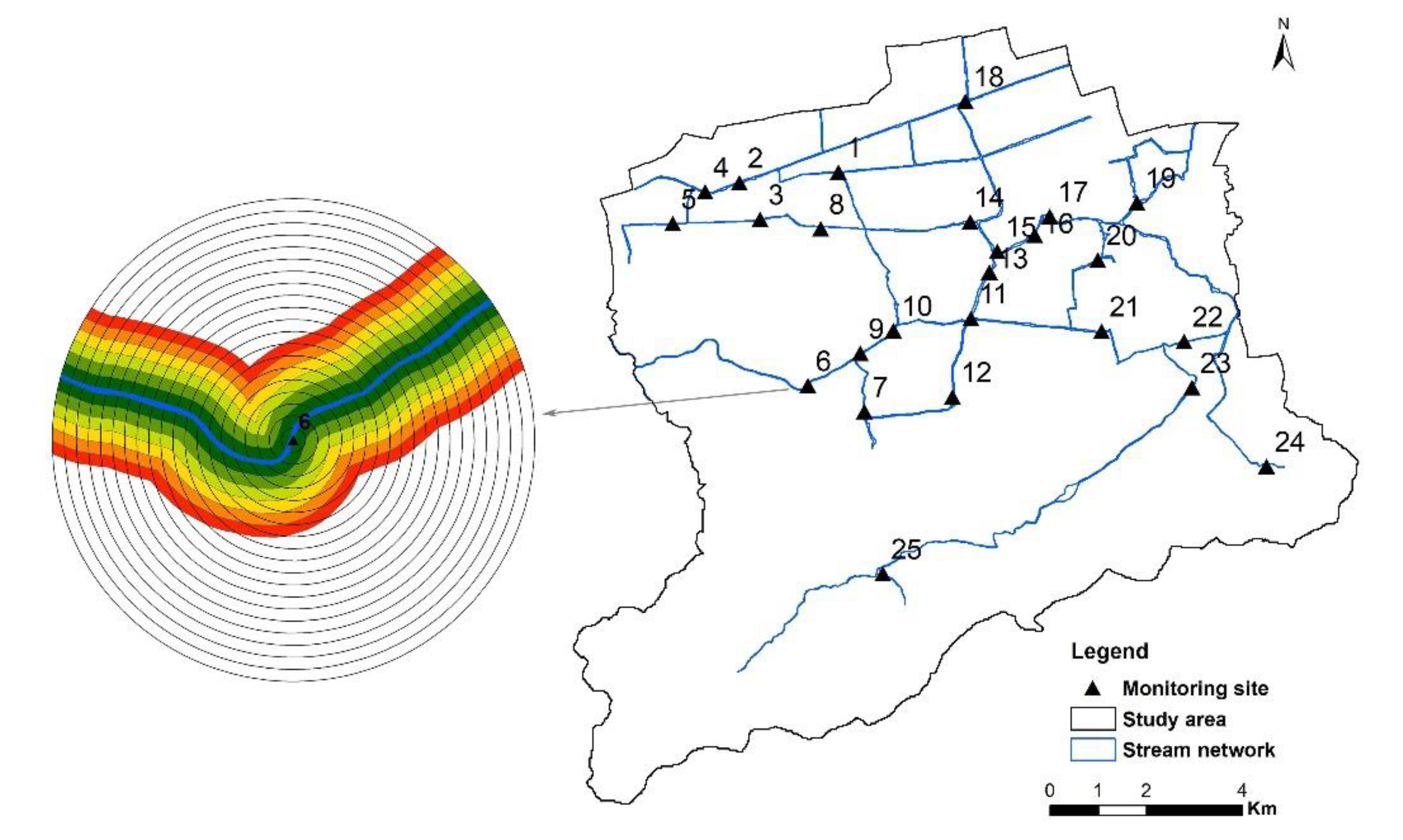
2.1. Study Area

Hangzhou City is a rapidly urbanizing city in the Yangtze River Delta in China (Figure 1). The study area is located in the west of Hangzhou, Zhejiang Province, which is a geographical unit that transitions from the low mountains and hills in the south to the northern plains. There are two large wetlands—the Hemu and Wuchang wetlands, in the study area, with intertwined stream networks. The study area has been experiencing intense urbanization during the past decade, and there have been increased contradictions between urban development and wetland protection in recent years. The study area is in the subtropical humid monsoon climate zone. The mountainous area is mainly composed by bedrock and residual slope deposits, and the plain area is mainly formed by Holocene sediments. The study area is about 120.19 km2, with most of the areas as plain and low-lying lands. The soils have been affected by human activities for centuries and can be categorized as anthrosols (FAO–UNESCO Soil Map of The World, 1988). The background concentrations of the heavy metals Cd, Pb, As, Ni, Cr, Zn and Cu in the plain area of the study area were 0.206, 38.2, 10.0, 41.1, 92.1, 110.0 and 40.8 (unit: mg/kg), respectively [35]. Except As, the concentrations of the other heavy metals were slightly higher than the corresponding values of the 1st class natural background given in the Soil Environment Quality Standard of China (GB15618-1995).

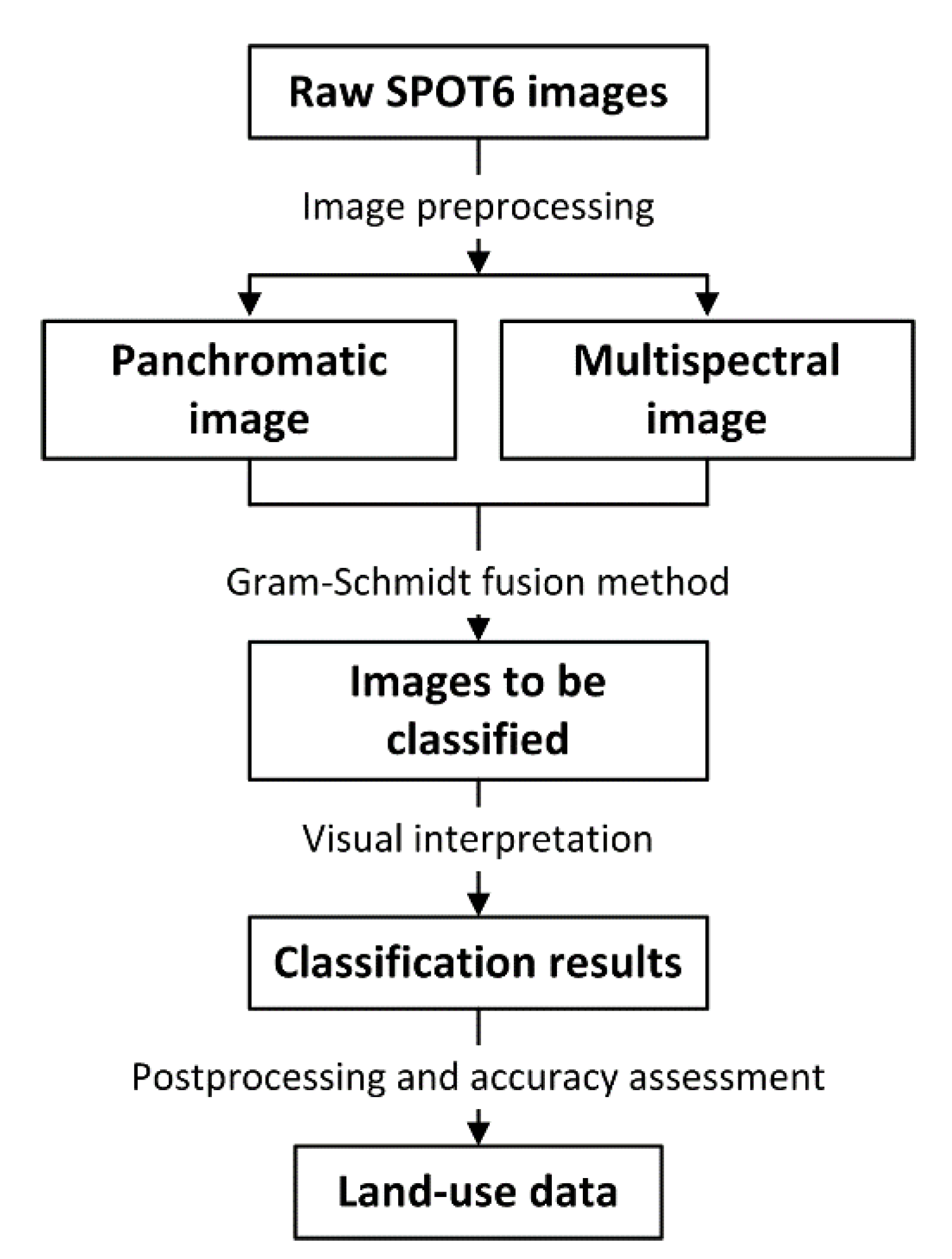
2.2. Land Use Information Extraction

One cloudless SPOT 6 image obtained on 26 October 2014 was used to extract the land use data over the study area. The SPOT 6 image had four multispectral bands and one panchromatic band with 1.5-m resolution. The ancillary data included ASTER DEM and field survey data.
The land use data was extracted using the following steps: (1) projection conversion and geometric correction of SPOT 6 image; (2) fusing the multispectral and panchromatic data using the Gram-Schmidt method (the fused image had a spatial resolution of 1.5 m with blue, green, red and near-infrared bands) and then (3) extracting the land use data by visual interpretation (Figure 2). The classification accuracy was evaluated using a stratified random sampling with reference to the ground-truth data collected in the field survey. The assessment results showed that the overall accuracy of the land use classification was 93%. We adopted a two-level classification schema from the Chinese Standard of Land Use Classification [36] and classified the lands into five Level I classes and 12 Level II classes (Table 1).

2.3. Water Sampling and Buffer Zone Delineation

The water quality of streams during the high water period is affected by the dual effects of land use, especially the construction land and cropland nonpoint sources, which could effectively reflect the content and intensity of human activities in the regional context [37,38,39,40]. The water quality sampling work at 25 stream sections was finished within one week when the stream flow was relatively stable during the local high-water period in June 2014 (Figure 3). The water quality parameters selected were total nitrogen (TN); total phosphorus (TP) and soluble heavy metals arsenic (As), copper (Cu), lead (Pb), chromium (Cr), cadmium (Cd), zinc (Zn), manganese (Mn) and nickel (Ni). The heavy metals selected in this study are the major heavy metals concentrated in the western plain areas of Zhejiang Province. Water samples were collected 0.3–0.5 m below the water surface from the middle of the stream using a 250-mL organic glass hydrophore. At each sampling site, three parallel samples were collected to avoid accidental error. The samples were stored in iceboxes during transport before water quality measurements were carried out in the laboratory. TP and TN were determined using the alkaline potassium persulfate digestion UV spectrophotometric method (GB11893-89, China National Standards) and the ammonium molybdate spectrophotometric method (GB11894-89, China National Standards), respectively. The heavy metal concentrations were determined using inductively coupled plasma optical emission spectrometry (ICP-OES, Thermo Fisher Scientific, Waltman, MA, USA). In addition, concentrations of chlorophyll a (TChla), including a chlorophyll a concentration of Cyanophyta (ChlaCyan), a chlorophyll a concentration of Chlorophyta (ChlaChlo) and a chlorophyll a concentration of Bacillariophyta and Dinophyta (ChlaBaci-Dino), were measured using a four-wavelength-excitation chlorophyll fluorometer (PHYTO-PAM Fa. Walz, Effeltrich, Germany), and each sample was sampled three times.
To explore the spatial scale effects of land use on water quality, two kinds of buffer scales were utilized, i.e., the riparian buffer zone along a specific stream and the circular buffer zone around the sampling point. In the literature, the buffer extent (width or radius) generally ranges from 50 to 1000 m, even 2000 m, according to the topography or sampling density in a case-specific manner, and the intervals between neighboring buffer zones are usually 50 to 100 m [28,41,42]. In this study, a series of buffers with varying widths/radiuses were tested to screen the optimal buffering schema. For the circular buffer scale, 20 buffering zones with radiuses ranging from 50 to 1000 m and an interval of 50 m were created around each sampling point. For the riparian buffer scale, six total buffering zones with widths ranging from 50 to 300 m with an interval of 50 m were created for each specific stream with a sampling point (Figure 3).

2.4. Landscape Metrics

It is acknowledged that there are correlations between regional landscape patterns and the hydrological, physical, chemical and biological indicators of a specific stream system [20,43,44,45]. We selected four categories of landscape metrics, i.e., fragmentation, dominance, connectedness and aggregation and shape complexity, to study the sensitivity of water quality on land use patterns at the class levels (Table 2).

2.5. Statistical Analysis

The correlations between the areas of each land use type and water quality at different spatial scales were analyzed. The Shapiro-Wilk test showed that some land uses and water quality data at certain buffering scales/sampling points did not follow the normal distribution, so we used the Spearman rank correlation, a nonparametric rank-based method which makes no assumption about the distribution of data, in the following analysis.
We also analyzed the relationships between water quality and land use patterns with a multivariate approach. The detrended correspondence analysis (DCA) was applied to evaluate the gradient length of the water quality data and revealed the existence of short gradients less than 3 standard deviations, so the redundancy analysis (RDA) was utilized to explore the relationships among water quality and land use pattern parameters, i.e., the species and environmental variables at the RDA context, respectively. A Monte Carlo permutation test (499 permutations) was used to determine the statistical validity of the RDA, and the significant explanatory variables were selected [46]. The RDAs were performed using the CANOCO 4.5 program.

3. Results

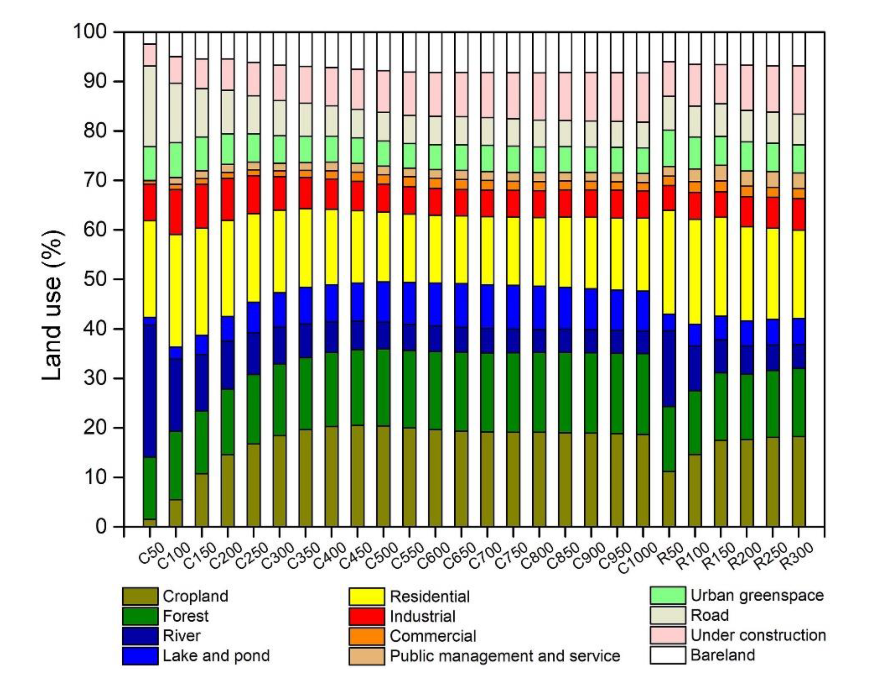
3.1. Land Use Patterns

As shown in the land use map of the study area (Figure 4), the forest land is concentrated in the southern mountain area; the lake and pond scattered in the central part of the study area (mainly concentrated in the Hemu and Wuchang wetlands) featured by a dense stream network, ponds and broken forest plots; the cropland concentrated in the north-central area; the industrial land mainly distributed in the north, west and south areas in a state of agglomeration and the large chunks of residential land mainly scattered along the major traffic roads at the eastern and southern areas, as well as the western area.
Figure 5 shows the average composition of land uses at each buffer scale. Overall, the ratios of the pervious surface and impervious surface were roughly equal. The agricultural, forest and residential lands were the dominant land uses. For each buffer zone, the buffer area and the areas of each land use were calculated, respectively. We summed up the areas of each land use in all buffer zones and calculated the ratios of the total areas of each land use to the total area of all the buffers. The following are the results for each land use. The ratios of the total area of the agricultural, forest and residential lands to the total area of all the buffers were 45% and 52% for the circular and riparian buffers, respectively; the ratios of the three land uses were 16.2%, 13.3% and 19.6%, respectively, at the riparian buffer scale, slightly higher than the corresponding ratios, i.e., 15.8%, 12.1% and 16.8% at the circular buffer scale. Taking the road, under construction and industrial land uses as a whole, the ratios were 25.5% and 20.8% for the circular and riparian buffers, respectively. The ratios of river, urban greenspace, lake and pond and bareland were all about 25% at the circular and riparian buffer scales. The commercial and public management and service had the smallest land areas, and the ratios at both buffering schemas were less than 5%.

3.2. Characteristics of Water Quality

The water quality analysis results of the sampling points are presented in Table S1 in the Supplementary Materials. The statistical analysis of the water quality parameters of the 25 river sections is shown in Table 3. The mean values of these parameters were compared with two Chinese national standards of water quality, i.e., the Environmental Quality Standards for Surface Water (EQSSW) (GB3838-2002, State Environmental Protection Administration of China) and the Sanitary Standards for Drinking Water Quality (SSDWQ) (GB 5749-2006). According to the EQSSW, the water quality is classified into five classes; the higher the class, the worse the water quality. Since Mn and Ni are not listed in the EQSSW, we referred the corresponding thresholds listed in the SSDWQ.
The average concentrations of the TN and TP exceeded the Class V surface water concentration limits, i.e., 2.0 and 0.4 mg/L for the TN and TP, respectively. For the TN, there were 16% and 80% sampling points, except No. 19 (Class IV), that were Class V and beyond; for the TP, there were 12%, 24%, 8% and 52% sampling points in Class III, IV, V and beyond, respectively, except No. 25 (Class II). The heavy metals at most of the sampling points were far below the surface water concentration limit of Class I or the limits in the SSDWQ, except No. 16 with Cr in Class II and No. 3 with Mn over the limits in the SSDWQ. Additionally, there were 40%, 84% and 92% sampling points that detected no Ni, Cd and Zn, respectively; all sampling points detected no Cu.
The mean concentrations of ChlaCyan, ChlaChlo and ChlaBaci-Dino were 8.39, 63.56 and 25.04 µg/L, respectively. The ChlaBaci-Dino in the Hemu and Wuchang wetlands were higher than the other areas. The mean value of TChla was 96.99 µg/L, a typical eutrophic water quality according to the Organization for Economic Co-Operation and Development (OECD) eutrophication evaluation criteria [47]. It was noted that there were 64% sampling points that detected no ChlaCyan.

3.3. Land Use Types and Water Quality

The correlation analysis showed that the nutrient concentration parameters, i.e., TN and TP, had certain correlations with the land use area at different buffer scales (Table S3 in the Supplementary Materials). Under the circular buffer scale, the TN had significant positive correlations with land areas of industrial, road, urban greenspace and commercial land uses, respectively. Specifically, the TN had significant positive correlations with commercial and urban greenspace land use areas at relatively small buffer scales ranging from 50–100 m and 50–400 m, respectively. The TN also had significant positive correlations with the industrial land use areas at relatively large buffer scales (450–1000 m), whilst the TN significantly positively correlated with the road areas at all buffer scales (50–1000 m). On the contrary, the TN had negative significant correlations with the areas of forest, lake and pond (hereafter referred to as wetland) and river land uses. For forests, the significant correlations could be observed at buffer scales ranging from 50–250 m, while, for the river as well as wetland, the ranges were 450–1000 m and 700–1000 m, respectively (Figure 6). Compared with the TN, there were less land uses that significantly correlated with the TP. At relatively large buffer scales, e.g., 650–750 m and 550–1000 m, the TP showed significant positive correlations with the areas of residential and industrial land uses, respectively, while, at small buffer scales (e.g. 50–100 m), the TP had significant positive correlations with commercial land areas (Figure 7). Under the riparian buffer scales, the TN was significantly negatively correlated with the forest areas, while the TP was significantly positively correlated with the areas of urban greenspaces.
The correlation analysis between the algae biomass and land use areas showed that the TChla and ChlaBaci-Dino had significant correlations with land uses at certain buffer scales (Table S4 in the Supplementary Materials). Under the riparian buffer scales, the TChla had significant positive correlations with the areas of river, wetland, industrial, urban greenspace, road and under construction land uses (Figure 8); the ChlaBaci-Dino had significant positive correlations with the areas of river, wetland and residential land uses (Figure 9). Under the circular buffer scale, the ChlaBaci-Dino showed significant positive correlations with the areas of forest, river and wetland at the ranges of 100–300 m, 50–1000 m and 150–1000 m, respectively, as well as negative correlations with the urban greenspace and road areas at the ranges of 650–1000 m and 150–1000 m, respectively. In addition, we found that the areas of wetland and road both had significant positive correlations with the ChlaChlo. Since most of the sampling points detected no Cyanophyta, no further analysis was carried out for this parameter.
The heavy metal concentrations also showed significant correlations with the areas of different kinds of land uses (Table S5 in the Supplementary Materials). For example, Cr and Ni had significant positive correlations with the area of industrial land, Mn and Ni both showed significant positive correlations with the areas of road and urban greenspace, As and Mn had significant positive and negative correlations with the agricultural land area, respectively and Cr and Pb had similar correlations with residential land areas; in addition, Pb also had significant positive correlations with the areas of wetland as well as the residential land uses and a significant negative correlation with the under construction land area. Since most of the sampling points did not detect Cd, Cu and Zn, no further analysis on these heavy metals was carried out.

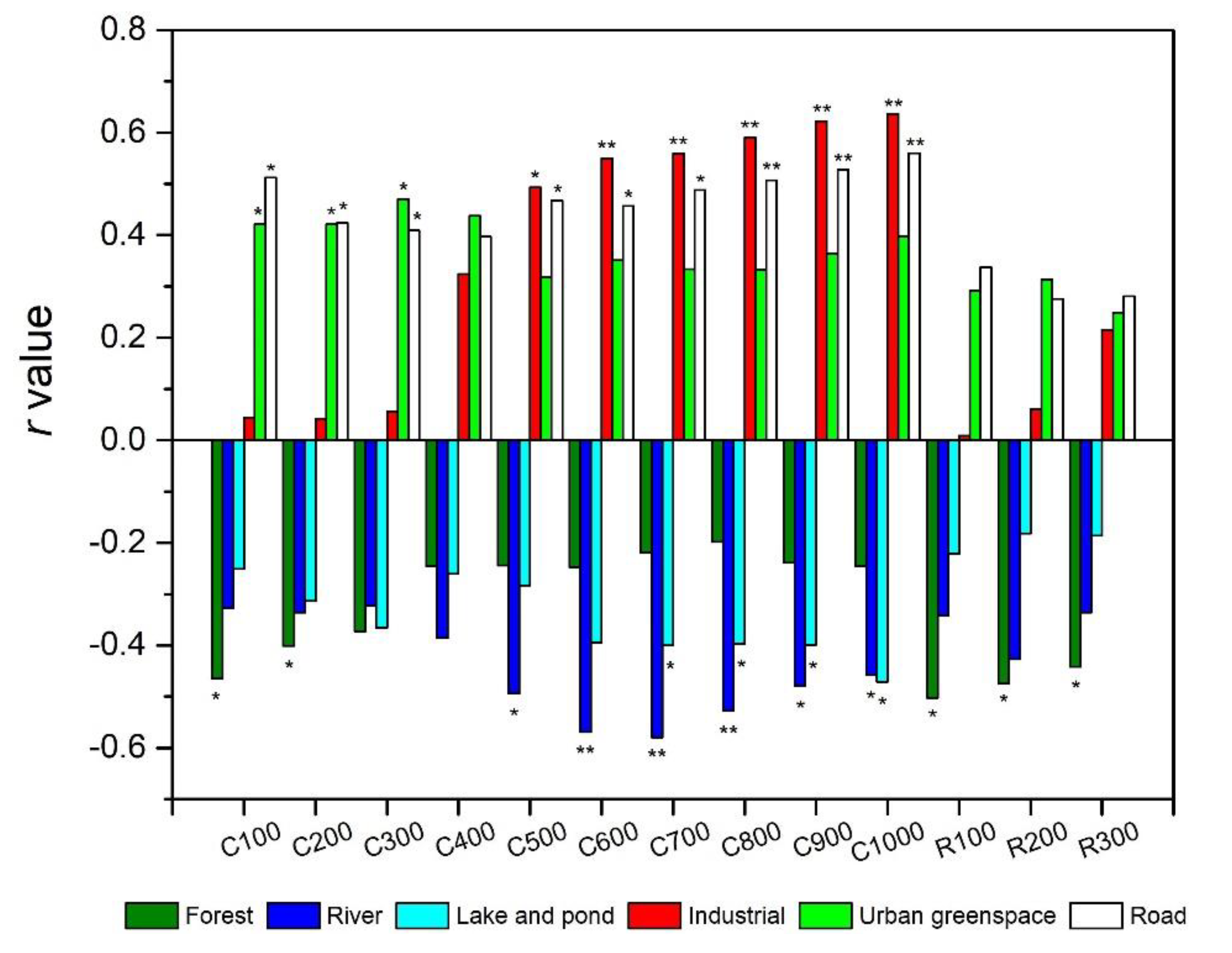
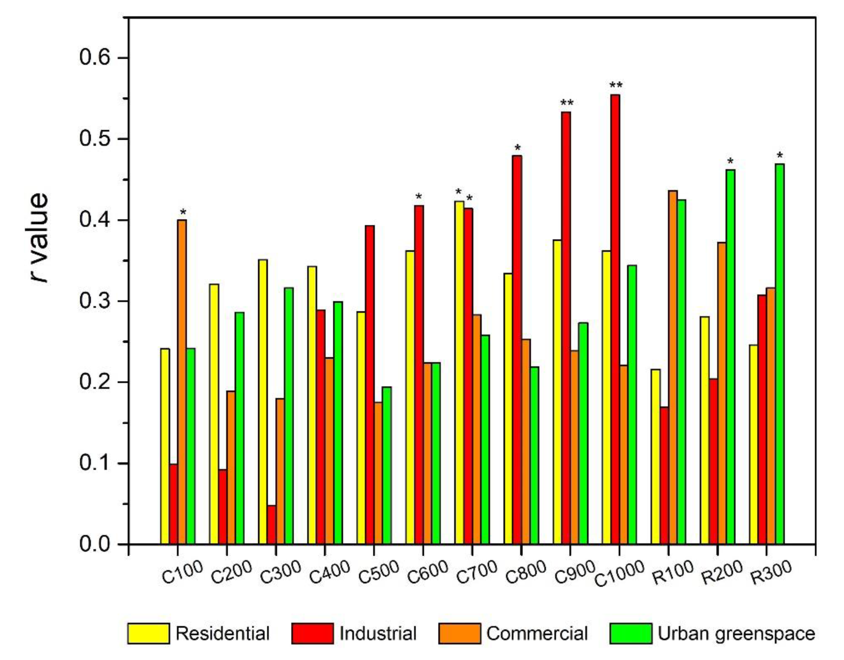
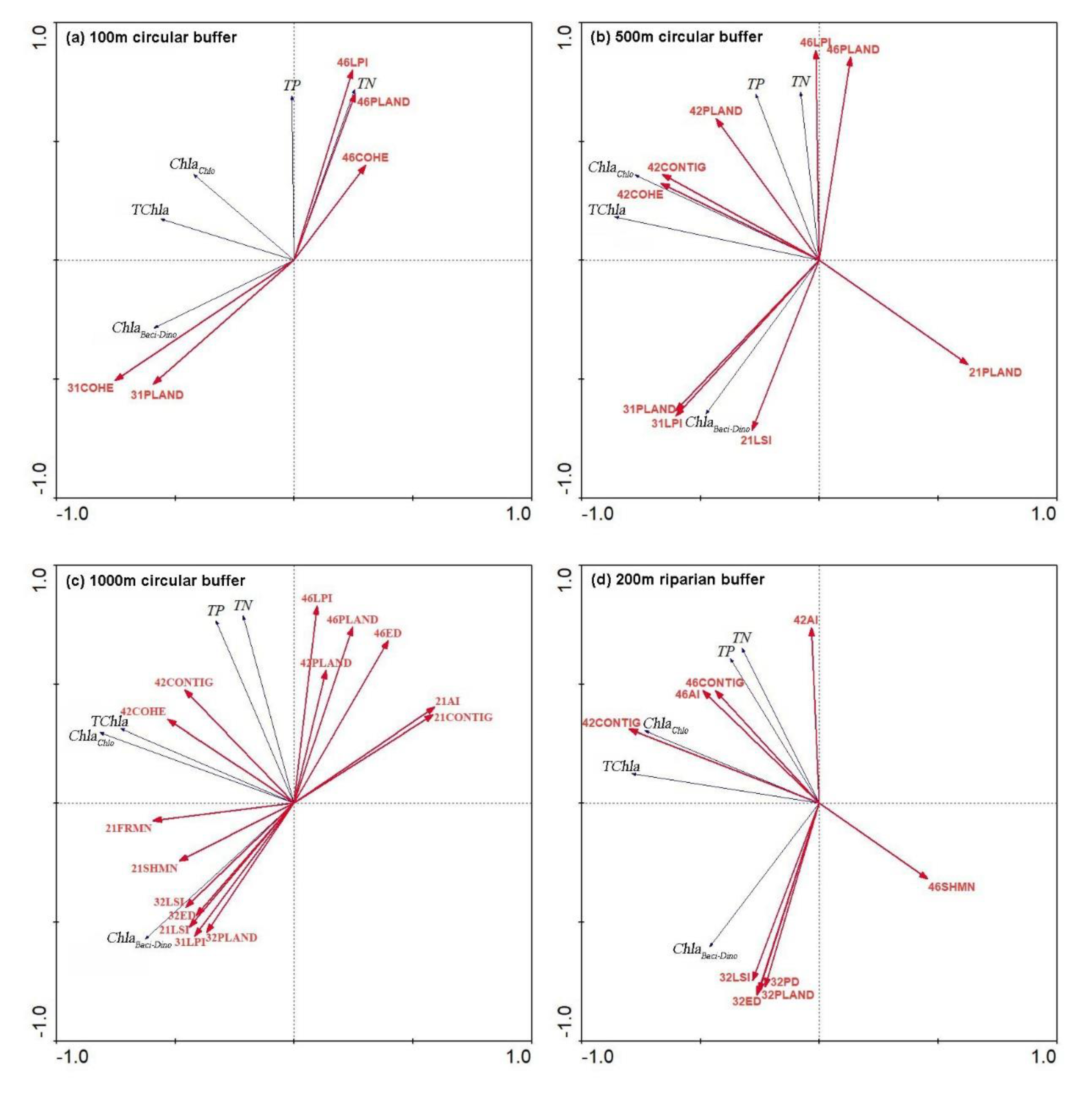
3.4. Land Use Patterns and Water Quality

We did a RDA at several typical buffer scales, i.e., 100, 500 and 1000 m, for the circular buffer and 200 m for the riparian buffer, respectively. The percentages of variance explained by the ordination axis are shown in Table 4. The RDA ordinations showed that there were statistically significant relationships between water quality and different numbers of explanatory variables, i.e., 5, 9 and 15 at 100, 500 and 1000-m circular buffer scales, respectively; at each scale, the landscape metrics could explain 39.5%, 71.7% and 80.9% of the variations in water quality, respectively. For the 200-m riparian buffer scale, there were statistically significant relationships between water quality and nine explanatory variables, and 60.1% of the variation in water quality could be explained by these variables. More than 40% water quality variation was explained by the first two axes, in which the first axis explained about twice as much as the second axis.
Figure 10 shows ordination diagrams derived from the RDA using water quality variables and significant explanatory variables for the four typical buffer scales. Under all scales, the first axis represents variables related with eutrophication, which was mainly related to the industrial land use. The second axis consistently displayed a gradient of nutrients, which was mainly positively correlated with roads and negatively correlated with wetlands. Particularly, the LPI and PLAND of roads were positively correlated with the TN and TP, whilst negatively correlated with ChlaBaci-Dino at 100, 500 and 1000-m circular buffer scales. Under 500 and 1000-m circular buffer scales, the PLAND of industrial land use was positively correlated with the TN and TP; except the TN and TP, the landscape metrics COHE and CONTIG were also positively correlated with the TChla and ChlaChlo. The CONTIG and AI of the road and industrial land uses were positively correlated with the TP, TN, TChla and ChlaChlo, whilst negatively correlated with the ChlaBaci-Dino at 200-m the riparian buffer scale. The SHMN of the roads was negatively correlated with the TP, TN, TChla and ChlaChlo.
The PLAND and LPI of the rivers were positively correlated with the ChlaBaci-Dino, whilst negatively correlated with the TN and TP at 100, 500 and 1000-m circular buffer scales. The PLAND, LSI and ED metrics of the wetlands were positively correlated with the ChlaBaci-Dino, while negatively correlated with the TN and TP at the 1000-m circular buffer scale and 200-m riparian buffer scale, respectively.
The PLAND of the forest land use was negatively correlated with the TN, TP, TChla and ChlaChlo, and the LSI was positively correlated with the ChlaBaci-Dino but negatively correlated with the TN and TP at the 500-m circular buffer scale. The FRMN, SHMN and LSI metrics of the forest land use were positively correlated with the ChlaBaci-Dino, ChlaChlo and TChla, but the AI and CONTIG were negatively correlated with these three water quality parameters at the 1000-m circular buffer scale.

4. Discussion

4.1. Water Pollution in Urbanized Areas

The land use pattern in the study area was mainly dominated by the urbanization process. The proportion of the impervious surface area was over 50% if adding up all the buffer zones used in this study—of which, the proportions of the residential, under construction, road, industrial, commercial and public management and service land uses decreased in turn (Figure 4). The less proportion of the commercial, as well as the public management and service land use, areas, compared with that of the residential land, suggested that the study area was still in the suburban urbanization process. It has been acknowledged that the early stages of rapid urbanization are often the beginning of the accelerated deterioration of urban surface water environments [48]. In the context of rapid urbanization, the TN and TP in stream water usually originated from industrial, living and agricultural activities [49,50]. The sampling data showed that the variations of water quality data were relatively large, and the concentrations of TN and TP were much higher than the Class V thresholds defined in the EQSSW (Table 3), a typical heavily polluted stream water environment.

4.2. Effects of Land Uses Types on Stream Water Quality

4.2.1. Nutrient and Heavy Metal Concentrations

The construction land area was an important factor to explain the change of TN concentration in stream waters (Figure 6). Under the circular buffer scale, the industrial, commercial, road and urban greenspace land uses were the primary sources of nitrogen pollution, whilst the areas of forest, wetland and river had significant negative correlations with the TN, showing effective degradation and purification effects on nitrogen pollution [23,51,52,53,54]. If only considering the TN, more than 80% sampled streams were beyond Class V, and this could be closely related with the densely distributed industrial land in this region, and further, the associated pollution might have exceeded the pollution load capacity of local aquatic ecosystems.
Compared with the TN, the TP had relative weak correlations with particular land uses. We found the TP had significant correlation with the industrial land area but no significant correlations with the area of forest, as well as wetland (Figure 7). This suggests that the TN and TP might have varied sensitivities to land use patterns, and the TN might be a more sensitive indicator of land use changes. We suggested that the TN might be more heavily influenced by human activities coupled with specific land use patterns, while the TP might be more controlled by strong point source emissions and had relative weak correlations with land use changes [55,56].
There was uncertainty in the relationships between the cropland area and concentrations of the TN and TP. The cropland area negatively correlated with the TN and TP, but neither was statistically significant, so it was not an appropriate factor that can be closely related to the eutrophication of water quality in this study area, despite in some cases where the cropland area was proved to be a promising predictor [57,58]. More specifically, this uncertainty could be closely related with local topography, cultivation practices and fertilizer usages [59,60,61]. The densely distributed stream network, including numerous ponds, made this study area more like a wetland from the functional perspective, and this kind of special geographical environment may have greatly weakened the pollution concentration coming from agriculture.
Generally, the construction land is the main source of heavy metal pollution, while the forest and wetland could absorb and promote the transformation of heavy metals [58,62]. In this study, we found significant positive correlations between heavy metals (e.g., Ni) and the areas of industrial, road and urban greenspace land uses, including significant negative correlations with the forest area at certain buffer scales. Similar to the cases of the TN and TP, there were also uncertainties in correlations between heavy metals and the cropland area, and both positive and negative correlations could be found (e.g., As and Mn). It was noted that there were relationships hard to interpret between certain heavy metals and some specific land uses (e.g., wetland and residential land uses); we suggested that this might be connected with the regional background sources [63,64].
The urban greenspace is a kind of urban construction land with special ecological significance, but we found that the area of urban greenspace, similar to the road, usually had significant positive correlations with the TN, TP and Mn at multiple buffer scales. Considering that the study area was still in the process of rapid urbanization, large parts of the greenspace distributed along with the road and traffic facilities, so it could be a main sink of vehicle pollutant emissions.

4.2.2. Algae Biomass

The TN and TP showed close relationships with the algae biomass (Table S2 in the Supplementary Materials), as shown by the positive correlations with the TChla and ChlaChlo, respectively. However, the relationship between the algae biomass and land use pattern was still not straightforward. For example, it was not surprising that the TChla positively correlated with the areas of construction lands, i.e., the industrial, road, urban greenspace and under construction land uses, at the riparian buffer scales (Figure 8). However, our results showed that the TChla positively correlated with the wetland areas, which was against the common consensus that the wetlands, e.g., stream, as well as lake and pond, could reduce the concentration of the TN and TP. It was suggested that, except for the concentrations of the TN and TP, the structure and growth of algae can also be affected by multiple factors, e.g., the ratio between the TN and TP, water pH and dissolved oxygen [65,66].
It was noted that the ChlaBaci-Dino was not sensitive to the TN and TP (Table S2 in the Supplementary Materials), whilst it showed significant negative correlations with the areas of construction lands, i.e., road and urban greenspace, and significant positive correlations with the forest and wetlands areas (Figure 9). In terms of spatial distribution, the ChlaBaci-Dino in the central part of the study area (Hemu and Wuchang wetlands) was relatively higher (Figure S1 in the Supplementary Materials). We suggested that this anomaly might be caused by the specific community structure of the ChlaBaci-Dino in the study area [67]. The wetlands in the study area were mainly composed of the stream network and cropland with closed ponds at the interior, and the impact of this complex land use composition on the structure and stability of the algae community still needs further study.

4.3. Effects of Land Use Patterns on Stream Water Quality

The land use patterns could explain more than 40% variation in water quality at all spatial scales (Table 4). This confirmed that land use patterns had a strong impact on water quality in the study area. For example, we found that the TN and TP were positively correlated with landscape metrics of the PLAND, LPI, CONTIG, COHE and AI of the road and industrial land uses, whilst negatively correlated with the PLAND and LPI of the wetland and river land uses in the RDA (Figure 10). The literature also suggested that the PLAND, LPI and AI are influential metrics on water quality [38,43,68,69].
We found that the larger ED, or higher LSI of the wetland, both correlated with a larger ChlaBaci-Dino at the 1000-m circular buffer scale. In addition, the higher LSI, SHMN and FDMN or lower AI and CONTIG of the forest were also positively correlated with the ChlaBaci-Dino (Figure 10). This suggested that the ChlaBaci-Dino biomass may have close relationships with the complexity and fragmentation characteristics of land use composition, and it emphasized the importance of the spatial structure of land use in this kind of study.
It was noted that the percentages of the explained variations of water quality by the CONTIG and COHE (connectedness); PLAND and LPI (dominance) and SHMN, FAMN and LSI (complexity) were very close. This finding might be helpful in water quality management practices, in that different kinds of compositions of landscape metrics could have similar explanation capabilities in water quality variations.

4.4. Influence of Spatial Scale on Land Use-Water Quality Relationships

Our results showed that the response characteristics of stream water quality to land use were spatial scale-dependent. Under the circular buffer scale, the land use was more closely related with the TN, but the corresponding buffer scales varied with particular land uses (Figure 6). The forest and urban greenspace were more influential to the TN at small buffer scales, and there was a tendency that the correlations (positive) between the TN and industrial land area increased, whilst the correlations (negative) generally decreased with the areas of wetland and river as the buffer scales increased. This suggests that the TN and TP could be partially mitigated by a more rational spatial arrangement of the lands of industry and forest or wetlands [70,71]. We also found strong correlations between land use and algae biomass at the riparian buffer scales (Figure 8), and this implies that the riparian buffer zone could play a key role in the conservation of aquatic ecosystems [72].
The land use patterns also showed scale effects on the water quality in the study area. The variation in water quality explained by the landscape metrics increased with the increasing of the spatial scale, and the total explained variation was up to 80% at the 1000-m circular buffer scale (Table 4). It means that the land use pattern could have continuously improving explanatory capabilities on the water quality, and this finding is consistent with other studies [25,29,68]. In this study, the maximum buffer width was 1000 m to avoid overlap with the neighboring buffer zones, but it would be worth it to explore what would be the relationship if the buffer scale further increased if data allowed.

5. Conclusions

The construction land area was an important factor to explain the variation of the TN concentrations in stream water. At the circular buffer scales, the industrial, commercial, road and urban greenspace land use areas significantly positively correlated with the TN; whilst the forest, wetland and river land use areas had significant negative correlations with the TN. The response characteristics of the stream water quality to land use were spatial scale-dependent. Under the circular buffer scale, the TN was more closely related with the land use status, but the corresponding buffer scales varied with the particular land use types. The forest and urban greenspace were more influential to the TN at small buffer scales, whilst significant positive or negative correlations could be found between the TN and the areas of industrial land or the wetland and stream as the buffer scales increased. Therefore, it might be possible to more quantitatively manage the water environment by identifying the particular buffer scales that closely relate with specific water quality parameters, for example, a more rational spatial arrangement of the industry land at larger spatial scales and the forest at smaller spatial scales to mitigate the TN and TP. In addition, there were more relevant correlations between the land use and algae biomass at the riparian buffer scales, and this suggests that the riparian buffer zone could play a key role in the conservation of aquatic ecosystems.
The land use pattern was an important factor influencing the water quality. The variations in water quality explained by landscape metrics were greater than 40% at all circular and riparian buffer scales. The increased landscape metrics of dominance and connectedness and aggregation of the industrial and road land uses, as well as the decreased landscape dominance metrics of the wetland and river, were correlated with the increased TN and TP. The land use pattern showed a scale effect on the water quality. The variation in water quality explained by the landscape metrics increased with the increasing of the buffer size, and it implies that the land use pattern could have a closer correlation with the water quality at larger spatial scales. This suggests that more attention should be paid to the landscape patterns at relatively larger spatial scales in water environment management practices.

Supplementary Materials

The following are available online at https://www.mdpi.com/2073-4441/12/4/1123/s1, Figure S1: Spatial variation of the (a) TN, (b) TP, (c) TChla, (d) ChlaCyan, (e) ChlaChlo and (f) ChlaBaci-Dino. The range of the corresponding concentration values were classified into six classes based on the natural breaks method. Table S1: Water quality analysis results of the sampling points. Table S2: Correlation coefficients between the stream nutrient concentration, heavy metals and algal biomass based on a Spearman’s rank order correlation analysis. Table S3: Correlations between the TN/TP and land uses at different spatial scales based on a Spearman’s rank correlation coefficient. Table S4: Correlations between the TChla, ChlaChlo, ChlaBaci-Dino and land use at different spatial scales based on a Spearman’s rank correlation coefficient. Table S5: Correlations between heavy metal concentrations and land uses at different spatial scales based on a Spearman’s rank correlation coefficient.

Author Contributions

Conceptualization, Y.S., X.S., G.S. and T.H.; data curation, Y.S., X.S. and T.H.; formal analysis, Y.S. and X.S.; investigation, Y.S. and X.S.; methodology, Y.S., X.S., G.S. and T.H.; software, Y.S.; supervision, X.S. and G.S.; validation, G.S.; writing—original draft, Y.S. and writing—review and editing, X.S., G.S. and T.H. All authors have read and agreed to the published version of the manuscript.

Funding

This research was funded by the Natural Science Foundation of Zhejiang Province, China (grant number: LQ13C030007), Entrepreneurship and Innovation Project for High-level Overseas Returnees in Hangzhou City in 2019 and the Science and Technology Project of the Water Resources Department of Zhejiang Province (grant number: RC1810).

Conflicts of Interest

The authors declare no conflicts of interest.

References

  1. Vörösmarty, C.J.; McIntyre, P.B.; Gessner, M.O.; Dudgeon, D.; Prusevich, A.; Green, P.; Glidden, S.; Bunn, S.E.; Sullivan, C.A.; Liermann, C.R. Global threats to human water security and river biodiversity. Nature 2010, 467, 555–561. [Google Scholar] [CrossRef] [PubMed]
  2. Arnold, C.L., Jr.; Gibbons, C.J. Impervious surface coverage: The emergence of a key environmental indicator. J. Am. Plan. Assoc. 1996, 62, 243–258. [Google Scholar] [CrossRef]
  3. Giri, S.; Qiu, Z. Understanding the relationship of land uses and water quality in Twenty First Century: A review. J. Environ. Manag. 2016, 173, 41–48. [Google Scholar] [CrossRef] [PubMed] [Green Version]
  4. Dewan, A.M.; Yamaguchi, Y. Land use and land cover change in Greater Dhaka, Bangladesh: Using remote sensing to promote sustainable urbanization. Appl. Geogr. 2009, 29, 390–401. [Google Scholar] [CrossRef]
  5. Ren, W.; Zhong, Y.; Meligrana, J.; Anderson, B.; Watt, W.E.; Chen, J.; Leung, H.-L. Urbanization, land use, and water quality in Shanghai: 1947–1996. Environ. Int. 2003, 29, 649–659. [Google Scholar] [CrossRef]
  6. Chen, Q.; Mei, K.; Dahlgren, R.A.; Wang, T.; Gong, J.; Zhang, M. Impacts of land use and population density on seasonal surface water quality using a modified geographically weighted regression. Sci. Total Environ. 2016, 572, 450–466. [Google Scholar] [CrossRef] [Green Version]
  7. Tong, S.T.; Chen, W. Modeling the relationship between land use and surface water quality. J. Environ. Manag. 2002, 66, 377–393. [Google Scholar] [CrossRef]
  8. Deng, J.S.; Wang, K.; Hong, Y.; Qi, J.G. Spatio-temporal dynamics and evolution of land use change and landscape pattern in response to rapid urbanization. Landsc. Urban Plan. 2009, 92, 187–198. [Google Scholar] [CrossRef]
  9. Delphin, S.; Escobedo, F.; Abd-Elrahman, A.; Cropper, W. Urbanization as a land use change driver of forest ecosystem services. Land Use Policy 2016, 54, 188–199. [Google Scholar] [CrossRef] [Green Version]
  10. Göbel, P.; Dierkes, C.; Coldewey, W. Storm water runoff concentration matrix for urban areas. J. Contam. Hydrol. 2007, 91, 26–42. [Google Scholar] [CrossRef]
  11. McGrane, S.J. Impacts of urbanisation on hydrological and water quality dynamics, and urban water management: A review. Hydrol. Sci. J. 2016, 61, 2295–2311. [Google Scholar] [CrossRef]
  12. Kannel, P.R.; Lee, S.; Kanel, S.R.; Khan, S.P.; Lee, Y.-S. Spatial–temporal variation and comparative assessment of water qualities of urban river system: A case study of the river Bagmati (Nepal). Environ. Monit. Assess. 2007, 129, 433–459. [Google Scholar] [CrossRef] [PubMed]
  13. Booth, D.B.; Roy, A.H.; Smith, B.; Capps, K.A. Global perspectives on the urban stream syndrome. Freshw. Sci. 2016, 35, 412–420. [Google Scholar] [CrossRef] [Green Version]
  14. Zhang, Y.; Wang, X.-N.; Ding, H.-Y.; Dai, Y.; Ding, S.; Gao, X. Threshold Responses in the Taxonomic and Functional Structure of Fish Assemblages to Land Use and Water Quality: A Case Study from the Taizi River. Water 2019, 11, 661. [Google Scholar] [CrossRef] [Green Version]
  15. Brabec, E.; Schulte, S.; Richards, P.L. Impervious surfaces and water quality: A review of current literature and its implications for watershed planning. J. Plan. Lit. 2002, 16, 499–514. [Google Scholar] [CrossRef]
  16. Schiff, R.; Benoit, G. Effects of Impervious Cover at Multiple Spatial Scales on Coastal Watershed Streams 1. J. Am. Water Resour. Assoc. 2007, 43, 712–730. [Google Scholar] [CrossRef]
  17. Zampella, R.A.; Procopio, N.A.; Lathrop, R.G.; Dow, C.L. Relationship of Land-Use/Land-Cover Patterns and Surface-Water Quality in The Mullica River Basin. J. Am. Water Resour. Assoc. 2007, 43, 594–604. [Google Scholar] [CrossRef]
  18. Klein, R.D. Urbanization and stream quality impairment. J. Am. Water Resour. Assoc. 1979, 15, 948–963. [Google Scholar] [CrossRef]
  19. Dai, X.; Zhou, Y.; Ma, W.; Zhou, L. Influence of spatial variation in land-use patterns and topography on water quality of the rivers inflowing to Fuxian Lake, a large deep lake in the plateau of southwestern China. Ecol. Eng. 2017, 99, 417–428. [Google Scholar] [CrossRef]
  20. Alberti, M.; Booth, D.; Hill, K.; Coburn, B.; Avolio, C.; Coe, S.; Spirandelli, D. The impact of urban patterns on aquatic ecosystems: An empirical analysis in Puget lowland sub-basins. Landsc. Urban Plan. 2007, 80, 345–361. [Google Scholar] [CrossRef]
  21. Buck, O.; Niyogi, D.K.; Townsend, C.R. Scale-dependence of land use effects on water quality of streams in agricultural catchments. Environ. Pollut. 2004, 130, 287–299. [Google Scholar] [CrossRef]
  22. Johnson, L.; Richards, C.; Host, G.; Arthur, J. Landscape influences on water chemistry in Midwestern stream ecosystems. Freshw. Biol. 1997, 37, 193–208. [Google Scholar] [CrossRef]
  23. Sliva, L.; Williams, D.D. Buffer zone versus whole catchment approaches to studying land use impact on river water quality. Water Res. 2001, 35, 3462–3472. [Google Scholar] [CrossRef]
  24. de Mello, K.; Valente, R.A.; Randhir, T.O.; dos Santos, A.C.A.; Vettorazzi, C.A. Effects of land use and land cover on water quality of low-order streams in Southeastern Brazil: Watershed versus riparian zone. Catena 2018, 167, 130–138. [Google Scholar] [CrossRef]
  25. Zhou, T.; Wu, J.; Peng, S. Assessing the effects of landscape pattern on river water quality at multiple scales: A case study of the Dongjiang River watershed, China. Ecol. Indic. 2012, 23, 166–175. [Google Scholar] [CrossRef]
  26. Hurley, T.; Mazumder, A. Spatial scale of land-use impacts on riverine drinking source water quality. Water Resour. Res. 2013, 49, 1591–1601. [Google Scholar] [CrossRef]
  27. Zhang, W.; Li, H.; Sun, D.; Zhou, L. A statistical assessment of the impact of agricultural land use intensity on regional surface water quality at multiple scales. Int. J. Environ. Res. Public Health 2012, 9, 4170–4186. [Google Scholar] [CrossRef] [Green Version]
  28. Kolpin, D.W. Agricultural chemicals in groundwater of the midwestern United States: Relations to land use. J. Environ. Qual. 1997, 26, 1025–1037. [Google Scholar] [CrossRef]
  29. Zhao, J.; Lin, L.; Yang, K.; Liu, Q.; Qian, G. Influences of land use on water quality in a reticular river network area: A case study in Shanghai, China. Landsc. Urban Plan. 2015, 137, 20–29. [Google Scholar] [CrossRef]
  30. Shen, Z.; Hou, X.; Li, W.; Aini, G.; Chen, L.; Gong, Y. Impact of landscape pattern at multiple spatial scales on water quality: A case study in a typical urbanised watershed in China. Ecol. Indic. 2015, 48, 417–427. [Google Scholar] [CrossRef]
  31. Lewis, W.M., Jr.; Mccutchan, J.R., Jr. Ecological responses to nutrients in streams and rivers of the Colorado mountains and foothills. Freshw. Biol. 2010, 55, 1973–1983. [Google Scholar] [CrossRef]
  32. Elliott, J.; Jones, I.; Thackeray, S. Testing the sensitivity of phytoplankton communities to changes in water temperature and nutrient load, in a temperate lake. Hydrobiologia 2006, 559, 401–411. [Google Scholar] [CrossRef]
  33. Rimet, F. Recent views on river pollution and diatoms. Hydrobiologia 2012, 683, 1–24. [Google Scholar] [CrossRef]
  34. An, K.-J.; Lee, S.-W.; Hwang, S.-J.; Park, S.-R.; Hwang, S.-A. Exploring the non-stationary effects of forests and developed land within watersheds on biological indicators of streams using geographically-weighted regression. Water 2016, 8, 120. [Google Scholar] [CrossRef] [Green Version]
  35. Wang, Q.H.; Dong, Y.X.; Zhou, G.H.; Zheng, W. Soil geochemical baseline and environmental background values of agricultural regions in Zhejiang province. J. Ecol. Rural. Environ. 2007, 23, 81–88. (In Chinese) [Google Scholar]
  36. National Bureau of Standards. Current Land Use Classification (GB/T 21010-2017); China Quality and Standards Publishing & Media Co., Ltd.: Beijing, China, 2017. (In Chinese) [Google Scholar]
  37. Bu, H.; Wei, M.; Yuan, Z.; Wan, J. Relationships between land use patterns and water quality in the Taizi River basin, China. Ecol. Indic. 2014, 41, 187–197. [Google Scholar] [CrossRef]
  38. Ai, L.; Shi, Z.H.; Yin, W.; Huang, X. Spatial and seasonal patterns in stream water contamination across mountainous watersheds: Linkage with landscape characteristics. J. Hydrol. 2015, 523, 398–408. [Google Scholar] [CrossRef]
  39. Pan, Y.; Herlihy, A.; Kaufmann, P.; Wigington, J.; Van Sickle, J.; Moser, T. Linkages among land-use, water quality, physical habitat conditions and lotic diatom assemblages: A multi-spatial scale assessment. Hydrobiologia 2004, 515, 59–73. [Google Scholar] [CrossRef]
  40. Xu, J.; Jin, G.; Tang, H.; Mo, Y.; Wang, Y.-G.; Li, L. Response of water quality to land use and sewage outfalls in different seasons. Sci. Total Environ. 2019, 696, 134014. [Google Scholar] [CrossRef]
  41. Allan, J.D. Landscapes and Riverscapes: The Influence of Land Use on Stream Ecosystems. Annu. Rev. Ecol. Evol. Syst. 2004, 35, 257–284. [Google Scholar] [CrossRef] [Green Version]
  42. Damanik-Ambarita, M.N.; Everaert, G.; Goethals, P.L. Ecological models to infer the quantitative relationship between land use and the aquatic macroinvertebrate community. Water 2018, 10, 184. [Google Scholar] [CrossRef] [Green Version]
  43. Lee, S.-W.; Hwang, S.-J.; Lee, S.-B.; Hwang, H.-S.; Sung, H.-C. Landscape ecological approach to the relationships of land use patterns in watersheds to water quality characteristics. Landsc. Urban Plan. 2009, 92, 80–89. [Google Scholar] [CrossRef]
  44. Zhang, G.; Guhathakurta, S.; Dai, G.; Wu, L.; Yan, L. The control of land-use patterns for stormwater management at multiple spatial scales. Environ. Manag. 2013, 51, 555–570. [Google Scholar] [CrossRef] [PubMed]
  45. Zhang, X.; Liu, Y.; Zhou, L. Correlation analysis between landscape metrics and water quality under multiple scales. Int. J. Environ. Res. Public Health 2018, 15, 1606. [Google Scholar] [CrossRef] [PubMed] [Green Version]
  46. Ter Braak, C.J.; Smilauer, P. Canoco Reference Manual and User’s Guide: Software for Ordination, Version 5.0; Microcomputer Power: Ithaca, NY, USA, 2012. [Google Scholar]
  47. Vollenweider, R.A.; Kerekes, J.J. Eutrophication of Waters: Monitoring, Assessment and Control; OECD: Paris, France, 1982. [Google Scholar]
  48. Hwang, S.-A.; Hwang, S.-J.; Park, S.-R.; Lee, S.-W. Examining the relationships between watershed urban land use and stream water quality using linear and generalized additive models. Water 2016, 8, 155. [Google Scholar] [CrossRef] [Green Version]
  49. Tromboni, F.; Dodds, W. Relationships between land use and stream nutrient concentrations in a highly urbanized tropical region of Brazil: Thresholds and riparian zones. Environ. Manag. 2017, 60, 30–40. [Google Scholar] [CrossRef] [PubMed]
  50. Beaulac, M.N.; Reckhow, K.H. An examination of land use—Nutrient export relationships. J. Am. Water Resour. Assoc. 1982, 18, 1013–1024. [Google Scholar] [CrossRef]
  51. Paul, M.J.; Meyer, J.L. Streams in the urban landscape. Annu. Rev. Ecol. Syst. 2001, 32, 333–365. [Google Scholar] [CrossRef]
  52. Rodríguez-Romero, A.J.; Rico-Sánchez, A.E.; Mendoza-Martínez, E.; Gómez-Ruiz, A.; Sedeño-Díaz, J.E.; López-López, E. Impact of changes of land use on water quality, from tropical forest to anthropogenic occupation: A multivariate approach. Water 2018, 10, 1518. [Google Scholar]
  53. Matteo, M.; Randhir, T.; Bloniarz, D. Watershed-scale impacts of forest buffers on water quality and runoff in urbanizing environment. J. Water Resour. Plan. Manag. 2006, 132, 144–152. [Google Scholar] [CrossRef]
  54. Brogna, D.; Dufrêne, M.; Michez, A.; Latli, A.; Jacobs, S.; Vincke, C.; Dendoncker, N. Forest cover correlates with good biological water quality. Insights from a regional study (Wallonia, Belgium). J. Environ. Manag. 2018, 211, 9–21. [Google Scholar] [CrossRef] [PubMed] [Green Version]
  55. Caccia, V.G.; Boyer, J.N. Spatial patterning of water quality in Biscayne Bay, Florida as a function of land use and water management. Mar. Pollut. Bull. 2005, 50, 1416–1429. [Google Scholar] [CrossRef] [PubMed]
  56. Puckett, L.J. Identifying the major sources of nutrient water pollution. Environ. Sci. Technol. 1995, 29, 408A–414A. [Google Scholar] [CrossRef]
  57. Meador, M.R.; Goldstein, R.M. Assessing water quality at large geographic scales: Relations among land use, water physicochemistry, riparian condition, and fish community structure. Environ. Manag. 2003, 31, 0504–0517. [Google Scholar] [CrossRef]
  58. Lenat, D.R.; Crawford, J.K. Effects of land use on water quality and aquatic biota of three North Carolina Piedmont streams. Hydrobiologia 1994, 294, 185–199. [Google Scholar] [CrossRef]
  59. Casalí, J.; Gastesi, R.; Álvarez-Mozos, J.; de Santisteban, L.; de Lersundi, J.D.V.; Giménez, R.; Larrañaga, A.; Goñi, M.; Agirre, U.; Campo, M. Runoff, erosion, and water quality of agricultural watersheds in central Navarre (Spain). Agric. Water Manag. 2008, 95, 1111–1128. [Google Scholar] [CrossRef]
  60. Ding, J.; Jiang, Y.; Fu, L.; Liu, Q.; Peng, Q.; Kang, M. Impacts of land use on surface water quality in a subtropical River Basin: A case study of the Dongjiang River Basin, Southeastern China. Water 2015, 7, 4427–4445. [Google Scholar] [CrossRef] [Green Version]
  61. Skaggs, R.W.; Breve, M.; Gilliam, J. Hydrologic and water quality impacts of agricultural drainage. Crit. Rev. Environ. Sci. Technol. 1994, 24, 1–32. [Google Scholar] [CrossRef]
  62. Bai, J.; Yang, Z.; Cui, B.; Gao, H.; Ding, Q. Some heavy metals distribution in wetland soils under different land use types along a typical plateau lake, China. Soil Tillage Res. 2010, 106, 344–348. [Google Scholar] [CrossRef]
  63. Ouyang, W.; Wang, Y.; Lin, C.; He, M.; Hao, F.; Liu, H.; Zhu, W. Heavy metal loss from agricultural watershed to aquatic system: A scientometrics review. Sci. Total Environ. 2018, 637, 208–220. [Google Scholar] [CrossRef]
  64. Lindström, M. Urban land use influences on heavy metal fluxes and surface sediment concentrations of small lakes. Water Air Soil Pollut. 2001, 126, 363–383. [Google Scholar] [CrossRef]
  65. Smith, V.H. Low nitrogen to phosphorus ratios favor dominance by blue-green algae in lake phytoplankton. Science 1983, 221, 669–671. [Google Scholar] [CrossRef] [Green Version]
  66. Zelnik, I.; Balanč, T.; Toman, M.J. Diversity and Structure of the tychoplankton diatom community in the limnocrene spring Zelenci (Slovenia) in relation to environmental factors. Water 2018, 10, 361. [Google Scholar] [CrossRef] [Green Version]
  67. Teittinen, A.; Taka, M.; Ruth, O.; Soininen, J. Variation in stream diatom communities in relation to water quality and catchment variables in a boreal, urbanized region. Sci. Total Environ. 2015, 530, 279–289. [Google Scholar] [CrossRef] [PubMed]
  68. Ding, J.; Jiang, Y.; Liu, Q.; Hou, Z.; Liao, J.; Fu, L.; Peng, Q. Influences of the land use pattern on water quality in low-order streams of the Dongjiang River basin, China: A multi-scale analysis. Sci. Total Environ. 2016, 551, 205–216. [Google Scholar] [CrossRef]
  69. Uuemaa, E.; Roosaare, J.; Mander, Ü. Landscape metrics as indicators of river water quality at catchment scale. Hydrol. Res. 2007, 38, 125–138. [Google Scholar] [CrossRef]
  70. Wang, X. Integrating water-quality management and land-use planning in a watershed context. J. Environ. Manag. 2001, 61, 25–36. [Google Scholar] [CrossRef]
  71. Mander, Ü.; Tournebize, J.; Tonderski, K.; Verhoeven, J.T.; Mitsch, W.J. Planning and establishment principles for constructed wetlands and riparian buffer zones in agricultural catchments. Ecol. Eng. 2017, 103, 296–300. [Google Scholar] [CrossRef]
  72. Junior, R.F.V.; Varandas, S.G.; Pacheco, F.A.; Pereira, V.R.; Santos, C.F.; Cortes, R.M.; Fernandes, L.F.S. Impacts of land use conflicts on riverine ecosystems. Land Use Policy 2015, 43, 48–62. [Google Scholar] [CrossRef] [Green Version]
Figure 1. Locations of the study area.
Water 12 01123 g001
Figure 2. Technical schema in the land use data extracted from SPOT 6 images.
Water 12 01123 g002
Figure 3. Spatial distribution of surface water quality monitoring sites. The left subfigure shows the buffering schema, i.e., the circular buffer and riparian buffer, used in this study. The interval of the neighboring buffers is 50 m. The circular buffer is a series of buffers around the sampling point with radiuses ranging from 50 to 1000 m, and the riparian buffer is along the particular stream bank with distances ranging from 50 to 300 m.
Water 12 01123 g003
Figure 4. Land use map of the study area.
Water 12 01123 g004
Figure 5. Proportions of each land use at different buffer scales. The labels at the x-axis indicate different buffer zones for the circular and riparian buffer scales, respectively. The initial character “C” or “R” represents the circular or riparian buffer types, and the numerical values after that character means the corresponding buffer radius. For example, “C50” means a circular buffer with a radius of 50 m around a sampling point. Hereinafter, the same.
Water 12 01123 g005
Figure 6. Correlations between TN and the areas of particular land uses under the circular and riparian buffer scales at different spatial scales based on a Spearman’s rank correlation analysis. The one-asterisk (two-asterisk) superscripts denote above 90% (95%) confidence levels. Note that only the land uses that significantly correlated with the TN were shown.
Water 12 01123 g006
Figure 7. Correlations between TP and the areas of particular land uses under the circular and riparian buffer scales at different spatial scales based on a Spearman’s rank correlation analysis. The one-asterisk (two-asterisk) superscripts denote above 90% (95%) confidence levels. Note that only the land uses that significantly correlated with the TP were shown.
Water 12 01123 g007
Figure 8. Correlations between TChla and the areas of particular land uses under the circular and riparian buffering scales at different spatial scales based on a Spearman’s rank correlation analysis. The one-asterisk (two-asterisk) superscripts denote above 90% (95%) confidence levels. Note that only the land uses that significantly correlated with TChla were shown.
Water 12 01123 g008
Figure 9. Correlations between ChlaBaci-Dino and the areas of particular land use types under the circular and riparian buffering scales at different spatial scales based on a Spearman’s rank correlation analysis. The one-asterisk (two-asterisk) superscripts denote above 90% (95%) confidence levels. Note that only the land uses that significantly correlated with the ChlaBaci-Dino were shown.
Water 12 01123 g009
Figure 10. Biplots of water quality parameters (represented by dark blue lines) and landscape metrics (represented by red lines) within the circular buffers of 100 m (a), 500 m (b) and 1000 m (c) and the riparian buffer of 200m (d) according to the redundancy analysis (RDA). The length of the arrow represents the standard deviation of variables in the sorting space, and the direction indicates the change of gradient direction. The cosine values of the arrow and axis represent the correlation.
Water 12 01123 g010
Table 1. Land use classification scheme.
Level ILevel IIDescription
1 Cropland11 CroplandCultivated land
2 Forest21 ForestA large area dominated by trees
3 Water31 RiverNatural-flowing watercourse and artificial canal
32 Lake and pondlake, reservoir and pond
4 Construction land41 ResidentialHouses and apartment buildings
42 IndustrialLand and buildings used for manufacturing, logistics, warehouse and mining
43 CommercialHouses and buildings for businessman working, commercial retails, restaurants, lodging and entertainments
44 Public management and serviceLands used for administration, public services and municipal utilities, education and research
45 Urban greenspaceParks and greenspace lands used for entertainments and environmental conservations
46 RoadPaved roads including freeways, major and minor city roads
47 Under constructionUnder construction but not yet finished
5 Bareland51 BarelandBare soil and bare rock
Table 2. Description of the landscape metrics selected at the class levels.
AttributesName (Abbreviation)UnitDescription
FragmentationEdge density (ED)m/haTotal length of all edge segments divided by total area for the corresponding patch type
Patch density (PD)n/km2Number of patches of the corresponding patch type per unit area
DominancePercentage of landscape (PLAND)%Percentage of the landscape comprised of the corresponding patch type
Largest patch index (LPI)%Proportion of total area occupied by the largest patch of a patch type
Shape complexityMean shape index (SHMN)-Mean patch perimeter divided by the minimum perimeter of the corresponding land use area
Mean fractal dimension index (FDMN)-Sum of 2 times the logarithm of the patch perimeter divided by the logarithm of the total area for the corresponding patch type divided by the number of patches
Landscape shape index (LSI)-Perimeter-to-area ratio for the corresponding class, increasing with irregular shapes
Connectedness and aggregationContiguity index (CONTIG)-Assessing patch shapes based on the spatial connectedness of cells within a patch
Cohesion index (COHE)-Indicates the physical connectedness of the corresponding patch type
Aggregation index (AI)%Number of like adjacencies involving the corresponding class, divided by the maximum possible number of like adjacencies involving the corresponding land use type
Table 3. Statistics of the stream water quality parameters. TN: total nitrogen and TP: total phosphorus.
IndicatorMaximumMinimumMean (Std.)
TN (mg/L)31.691.346.46 (6.73)
TP (mg/L)2.800.090.61 (0.62)
As (μg/L)8.200.004.48 (2.28)
Cd (μg/L)1.000.000.10 (0.27)
Cr (μg/L)12.300.003.66(3.36)
Cu (μg/L)0.000.000.00 (0.00)
Mn (μg/L)676.400.0030.40 (134.80)
Ni (μg/L)1.700.000.32 (0.43)
Pb (μg/L)5.400.001.98 (1.43)
Zn (μg/L)2.000.000.13 (0.46)
ChlaCyan (μg/L) 1130.430.008.39 (26.52)
ChlaChlo (μg/L) 2233.290.0063.56 (69.46)
ChlaBaci-Dino (ug/L) 3138.740.0025.04 (31.18)
TChla (μg/L) 4328.842.0896.99 (83.75)
1 ChlaCyan: chlorophyll a concentration of Cyanophyta. 2 ChlaChlo: chlorophyll a concentration of Chlorophyta. 3 ChlaBaci-Dino: chlorophyll a concentration of Bacillariophyta and Dinophyta. 4 TChla: total chlorophyll a concentration.
Table 4. Variations in water quality explained by land uses and landscape metrics at different buffer scales in the redundancy analysis (RDA).
ScalesExplained Variation (%)Explanatory Variables Selected (p < 0.05)
Axis 1Axis 2All Axes
100-m circular buffer26.012.239.531COHE, 31PLAND, 46LPI, 46PLAND and 46COHE
500-m circular buffer43.925.271.621LSI, 21PLAND, 31LPI, 31PLAND, 42COHE, 42CONTIG, 42PLAND, 46LPI and 46PLAND
1000-m circular buffer47.423.780.921AI, 21CONTIG, 21FRMN, 21LSI, 21SHMN, 31LPI, 32ED, 32LSI, 32PLAND, 42COHE, 42CONTIG, 42PLAND, 46ED, 46LPI and 46PLAND
200-m riparian buffer38.220.360.132ED, 32PD, 32LSI, 32PLAND, 42AI, 42CONTIG, 46AI, 46CONTIG and 46SHMN
Notes: Landscape metrics include the edge density (ED), patch density (PD), percentage of landscape (PLAND), largest patch index (LPI), mean shape index (SHMN), mean fractal dimension index (FDMN), landscape shape index (LSI), contiguity index (CONTIG), cohesion index (COHE) and aggregation index (AI). The land use metrics refer to the following land use types, i.e., 11 (cropland), 21 (forest), 31 (river), 32 (wetland), 42 (industrial) and 46 (road). The p-values were derived from Monte Carlo permutation tests (499 permutations) of all of the canonical axes.

