1. Introduction
The dissolution of CO
in water slightly increases the density of water; e.g., [
1]. This can lead to an unstable layering of CO
-rich water with a higher density above water with lower density. Convective mixing characterized by protruding fingers is triggered after a certain onset time. In geological systems, we often see double-diffusive convective systems, where density differences typically arise from changes in the concentration of the dissolved components and from differences in temperature. For this study at atmospheric pressure, we focus on concentration-dependent processes by keeping the temperature constant, and consequently denote the process as density-driven or density-induced dissolution.
Convective dissolution is of practical importance in various technical and geological fields of research. One such field is CO
geological storage. The injection of supercritical CO
into a geological formation, e.g., a saline aquifer, typically leads to a buoyancy-driven segregation of the CO
and the brine. The CO
fluid density depends on the pressure and temperature in a reservoir and is often in the order of half the density of the brine. Thus, the CO
phase will end up in a stratum underneath a hydraulic barrier on top of the brine. Over time, CO
dissolves in the brine, increases the brine’s density, and triggers a fingering process, which eventually results in an enhanced dissolution and an effective vertical downward transport of CO
. This effect has already been discussed in early publications in the field of CO
geological storage, e.g., [
2,
3], and is denoted also as solubility trapping [
4]. On the subject of CO
geological storage, many publications are found on (in-)stability analyses and estimates for the time until the onset of fingering or the wave length of the fingering pattern in porous media, e.g., [
5,
6,
7,
8,
9], or the scaling with different dimensionless numbers, e.g., [
10]. High-resolution numerical studies on Darcy-type models for porous media also show that the spatial discretization length has to be very small relative to the scale of a typical storage reservoir in order for us to resolve onset time and fingering pattern correctly [
7,
11], making grid-converged results on large spatial scales practically infeasible. Therefore, more pragmatic approaches avoid the resolution of the fingers and employ effective rates, dependent on permeability; density difference as a function of CO
concentration and brine salinity; and fluid viscosity [
11]. An overview is given, for example, in the paper of Green and Ennis-King (2018) [
12].
This study is motivated by another problem, featuring similar processes of CO
density-driven dissolution but in a completely different context. Karstification is a field where CO
density-driven dissolution in a water body may play a role underestimated so far. Scherzer et al. (2017) [
13] formulated the concept of nerochytic (from Greek nerochytis = sink) speleogenesis which hypothesizes the density-driven dissolution of CO
from cave air with elevated CO
concentrations in the cave atmosphere in the water body to be a relevant mechanism for karstification. CO
density-driven dissolution might be a process that can be considered an essential supplement to common karstification models, since it could enrich water bodies with additional carbonic acid from cave air with its seasonal fluctuations in CO
concentrations. Thus, it would contribute to a perpetuation of the dissolution potential in the phreatic zone and consequently increase the dissolution rate of CaCO
there. In this context, we are interested in estimating the time-scales on which an enrichment of resting cave waters with dissolved CO
may take place. Furthermore, a quantitative understanding of the seasonal dynamics of CO
input to cave water may allow estimates on how significant this transport process might be for karstification. We consider numerical modeling as an appropriate tool for studying such effects over the relevant geological time-scales, including both the dynamics in flow and transport processes, and the chemistry of the CO
reacting with water to form carbonic acid and further upon dissolving calcium carbonate. Our vision is to develop and validate such a model; this study aims at contributing to it. The particular focus of the validation attempt is on the sinking velocity of the density-induced fingers, since, for the application we have in mind, it is far more important to capture the dynamics of the fingers during seasonal fluctuations in CO
concentrations rather than the onset time of the first fingers. According to [
14],
validation is the substantiation that a computerized model within its domain of applicability possesses a satisfactory range of accuracy consistent with the intended application of the model.
In other words, we consider validation to be the successful comparison of the simulation result with data from a well-controlled experiment. In this study, we present a first step towards this goal.
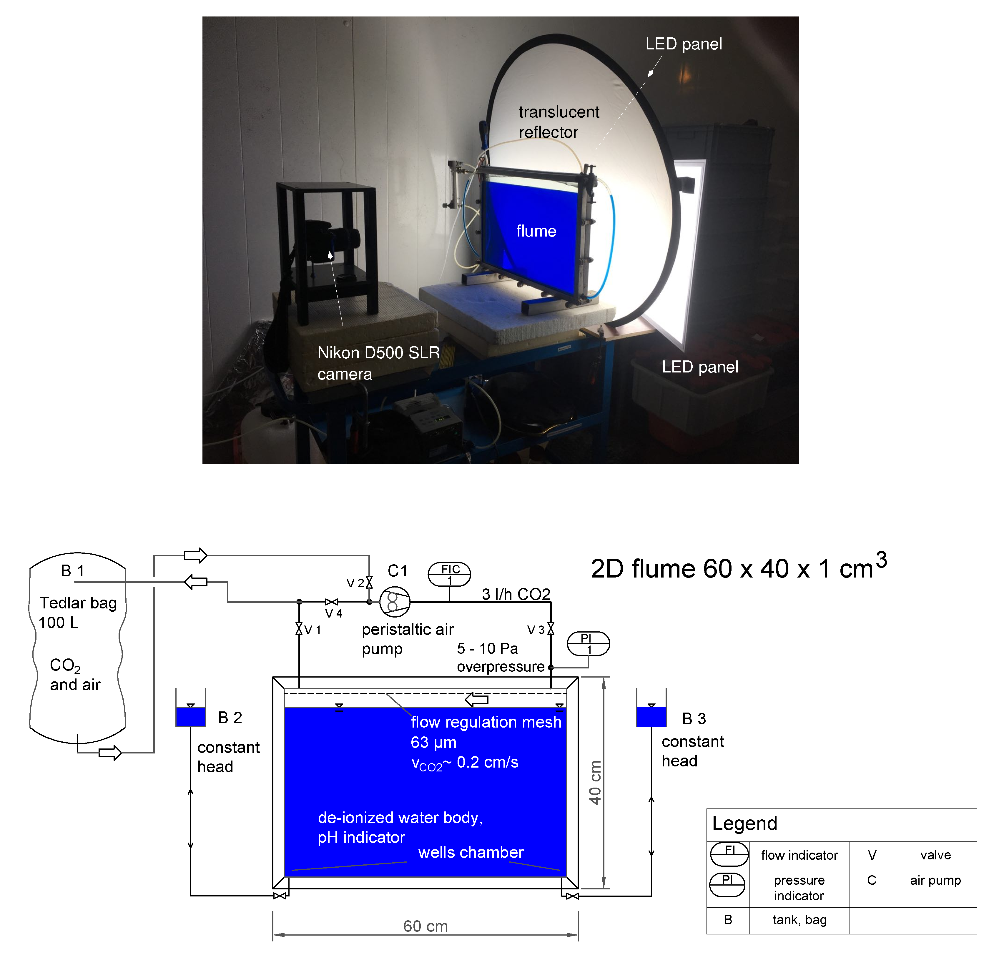
We set up a quasi-two-dimensional experiment in a laboratory flume with dimensions 60 cm × 40 cm × 1 cm, where we visualized density-driven dissolution of CO
using a pH-sensitive color indicator; see
Section 2.1. The data of onset time and evolving fingering pattern over time were then compared with the results of a numerical model that solves the Navier–Stokes equation with a density dependent on CO
concentration, and a transport equation for CO
including advective and diffusive terms. The model is presented in
Section 2.2 and the results and discussion of the comparison between the experiment and simulation are found in
Section 3 and
Section 4.
3. Results
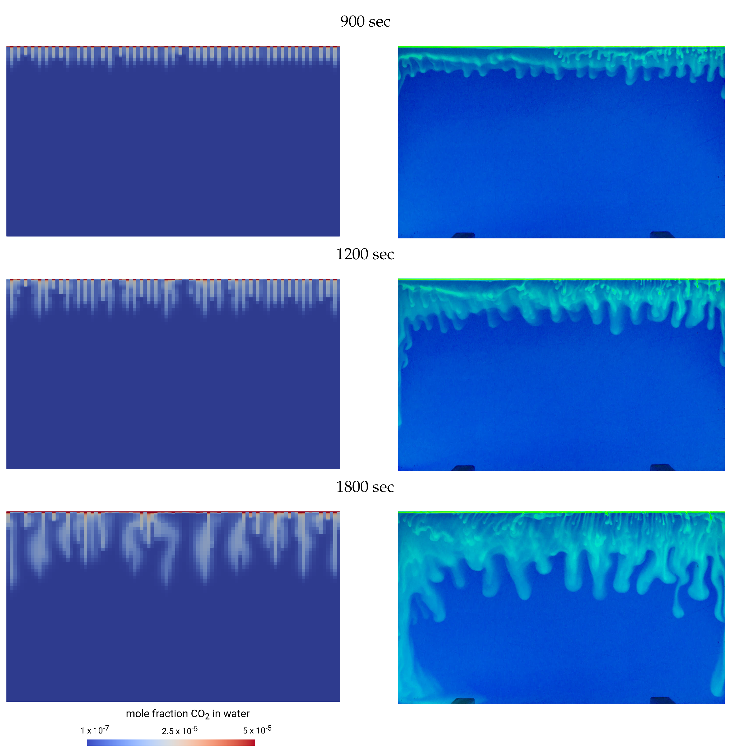
Figure 4 and
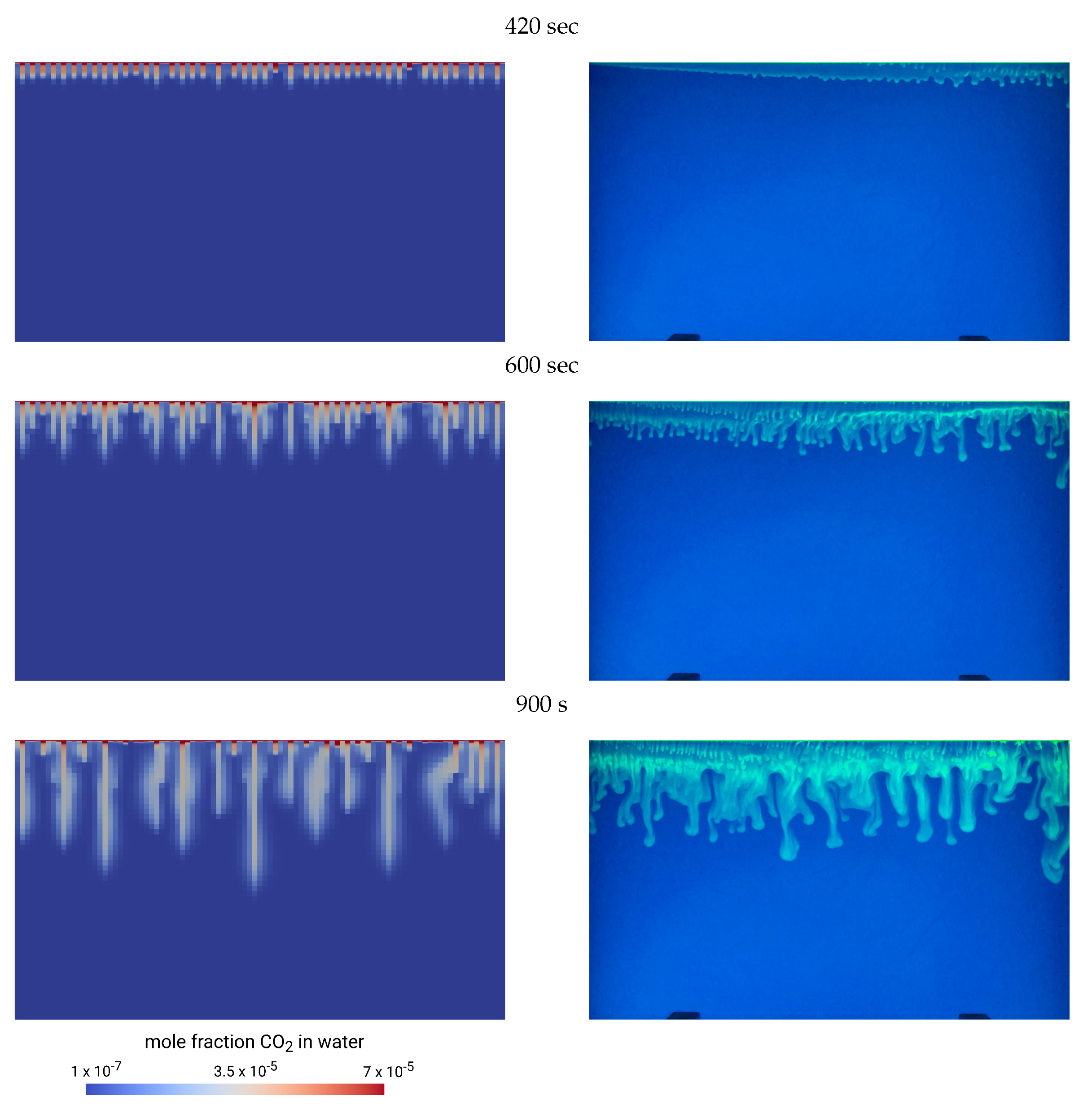
Figure 5 show the comparison between pseudo-3D numerical simulation results, obtained with the graded grid, and pictures taken at three different times during the experiments with
atm (
Figure 4) and with
atm (
Figure 5), both at 8 °C. The pseudo-3D approach is computationally as efficient as the 2D approach, and in terms of the relevant metrics, i.e., onset time and finger velocities, almost as “correct” as the 3D approach, as shown further below. Numerical results are displayed with a constant color legend for the mole fractions in all plots within each figure, but minimum/maximum values of CO
mole fraction differ from figure to figure. We did not attempt to derive reliable values of CO
concentrations from the photos, since this would have required a very costly calibration procedure, probably without much additional benefit for this study. The color indicator consumes some CO
before changing color. Therefore, we do not consider it appropriate to try to compare the very details between the numerical results and the photos. The color indicator might suppress the diffusive part of the processes, whereas we expect that the dynamics of the convective fingers are reasonable to compare. This is indeed confirmed by the comparison provided in
Figure 4 and
Figure 5 with a very satisfactory agreement between model results and experiments.
Experiments at 8 °C were successfully performed for 1 atm, 0.75 atm, 0.5 atm, 0.25 atm, and 0.05 atm. We also conducted two experiments at 20 °C at atm, 0.75 atm, and 0.5 atm. Without any fitting of parameters, the onset of instability is at about the same time in model and experiment when the graded grid is used. The same holds for the progress of the fingers. At later times, there is a tendency towards more disagreement between numerical results and experiments. The experimental fingers seem to get stuck or retarded after some time, and cease to show the same dynamics as the numerical fingers. The buffering by the color indicator probably hinders the visualization of the diffusive processes that tend to dilute the protruding fingers as they grow.
A full set of photos is provided in the
Supplementary Materials; it is representative of the experimental setups with 0.75 atm both at 8 °C and at 20 °C.
The initial dynamics are mainly determined by the evolving convective flow once the instability sets in. Therefore, as a criterion for model validation, we will compare the simulations and experiments with regard to the onset times and the velocities of the protruding fingers.
The 2D simulations neglect the third dimension, while the pseudo-3D model accounts for it phenomenologically by a drag term for wall friction. In fact, the 1 cm distance between that back and front plate has an influence on the dynamics, since no-slip conditions slow down the induced flow. Using
to estimate a permeability analogous to that in a porous porous medium yields a value of 8.3 × 10
m
. This is a relatively high value, and a Darcy model is therefore not appropriate since Reynolds numbers at typical finger velocities in this study are in the order of 1 or slightly higher; i.e., too high.
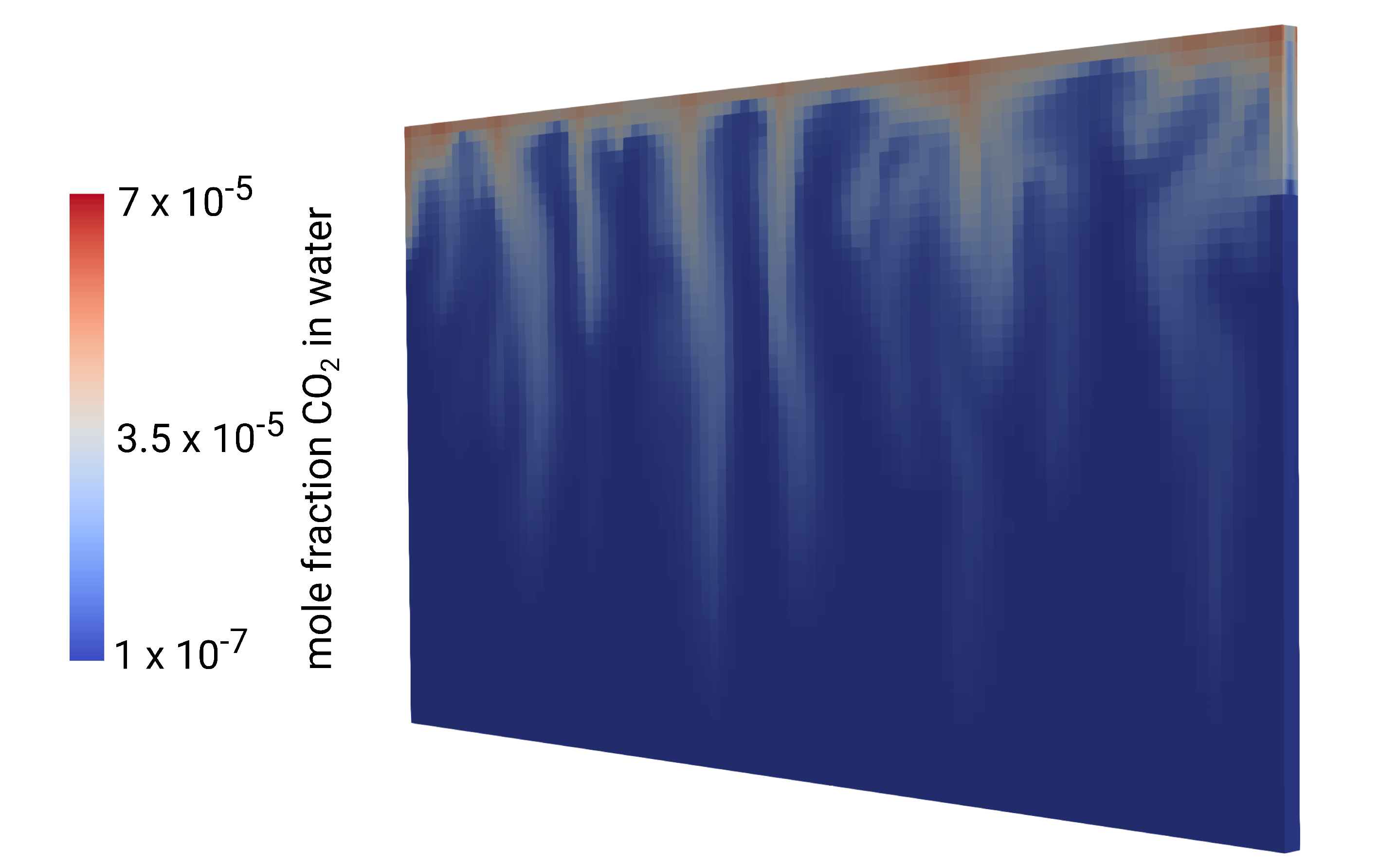
Figure 6 shows an exemplary snap-shot of a 3D simulation with
atm at 8 °C. It is clearly visible that the CO
concentrations accumulate at all no-flow boundaries. Thus, density differences are high there in particular, and the onset of fingering starts at the boundaries. This effect is not seen in the 2D and pseudo-3D simulations, while the images of the experiments confirm the accumulation of CO
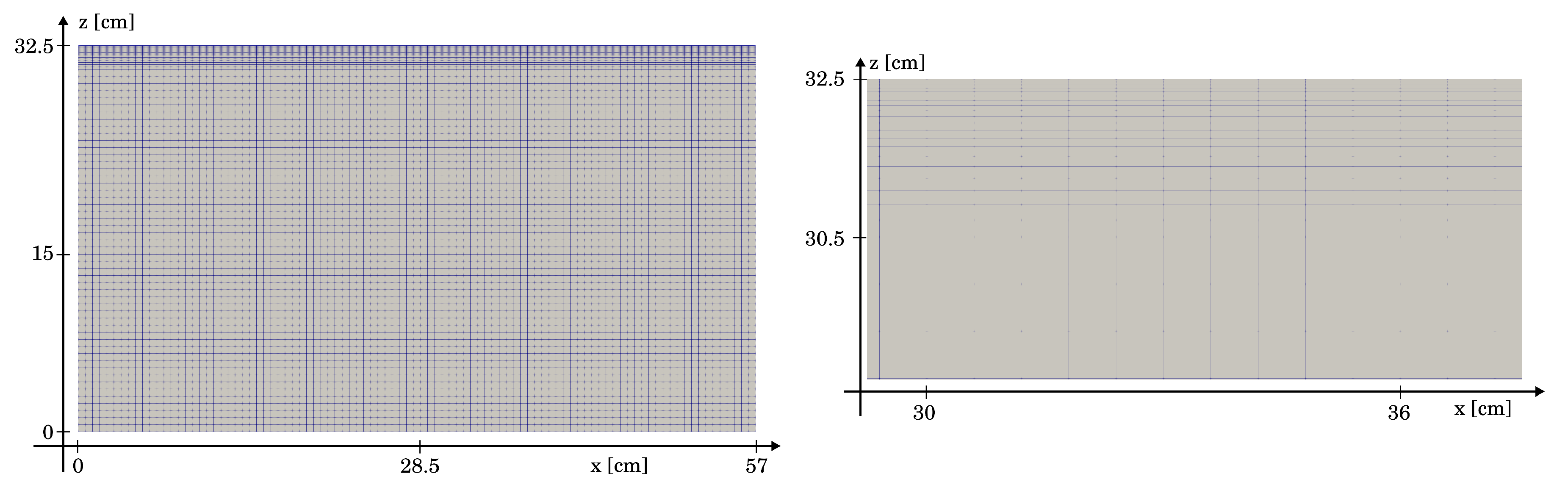
at the lateral boundaries. The grid resolution in the simulations is very high in the top few centimeters, and thus almost comparable with high-resolution studies; for example, [
7,
11]. We tested further grid refinement below the graded region only for the 2D simulations, but this did not further improve the mainly qualitative comparison with the experiments.
Onset times were determined in both simulation and experiment simply as those times when the initiation of fingers could be clearly discerned in the plots and images. Of course, this involves some uncertainty, but the overall significant uncertainties in the experiment justify this approach. Similarly, the wave lengths were “measured” from the finger tips observed in the simulations. We did not try to express the wave lengths in numerical values. A qualitative look at the images and comparison with the simulations shows similar behavior; see also
Figure 4 and
Figure 5. The onset times of the pseudo-3D simulations are summarized in
Table 2. 3D results and their evaluation were very similar and are omitted for the sake of brevity. The table further provides the values for the proportionality factor
as obtained by solving Equation (
9). The values are not constant, but rather differ over orders of magnitude; thus, they clearly indicate that the factors of influence in Equation (
9) do not cover all relevant processes properly.
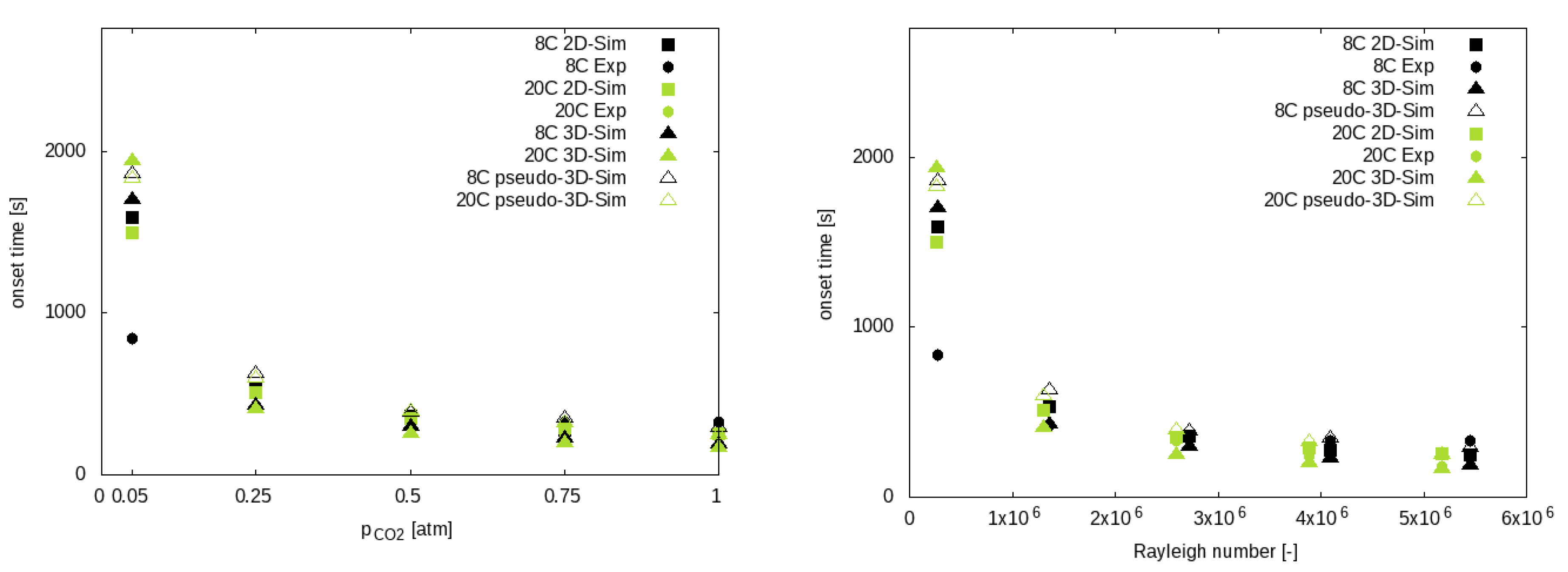
Figure 7 shows the onset times depending on the concentration of CO
in the atmosphere at the top boundary and depending on the Rayleigh number. The plots in
Figure 7 use model results from the graded grid. They show a clear and consistent tendency towards later onset for smaller CO
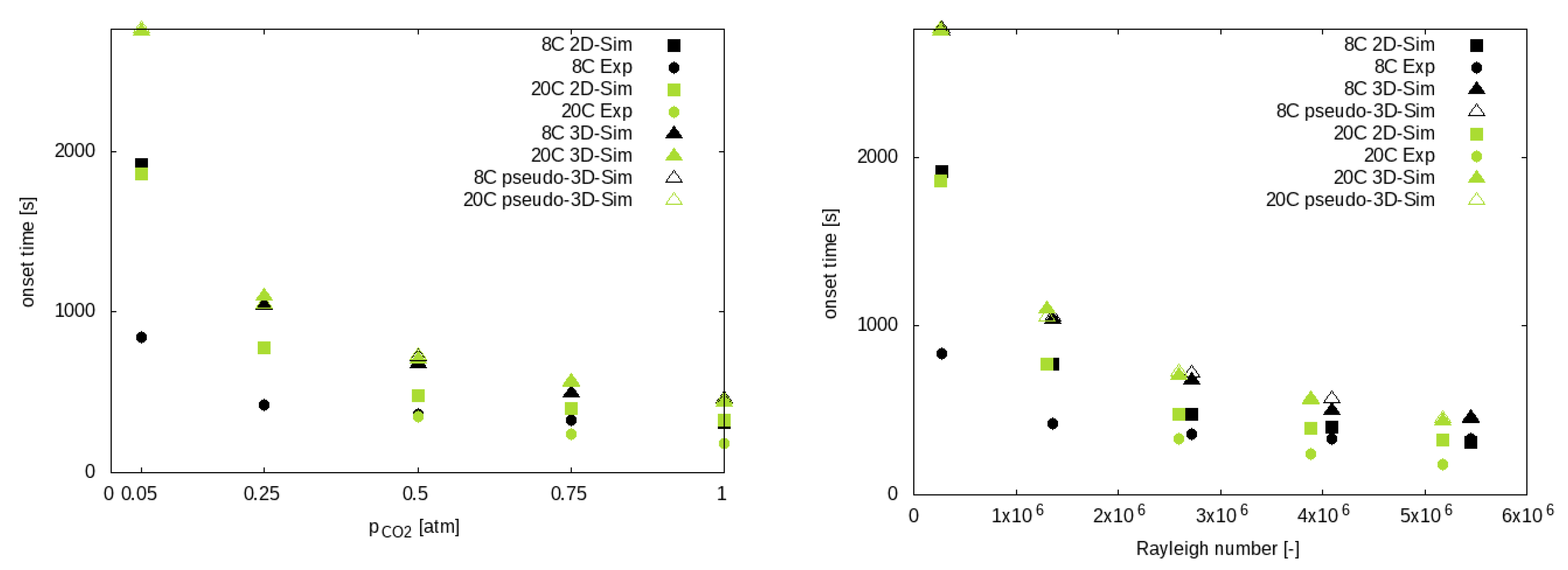
concentrations and smaller Rayleigh numbers. We can see the same tendency in the plots of
Figure 8, which uses the model results from the regular grid. The experimental onset times are in very good agreement with the simulations on the graded grid, except for the case with 0.05 atm where the experimental value at 8 °C is earlier than the models’. At 8 °C and 0.5 atm, for example, we see deviations from the experimental value of 0.8% higher for the 2D graded grid, 18% lower for the 3D graded, 7.5% higher for the pseudo-3D graded, 88% higher for the 3D regular, 33% higher for the 2D regular, and 99% higher for the pseudo-3D regular. Experimental results at 20 °C are not available for all CO
concentrations. While the results, both in the simulations and the experiments, did not show a strong influence of the temperature, we faced problems visualizing the fingers with the color indicator for higher temperatures and smaller CO
concentrations. The results on the regular grid do not match as well as those on the graded grid. Here, the 2D results seem to match better than the pseudo-3D and 3D. We argued above that pseudo-3D and 3D should be expected to be more realistic, since they consider wall friction. Therefore, further explanation is required to understand this effect. In fact, this depends on the implementation of the Dirichlet boundary condition for the CO
concentration at the top. Initially, we assumed that no dissolved CO
was present in the topmost cell. Therefore, at time zero, diffusion starts filling up the first cell and instability develops in terms of a growing density difference. The smaller the topmost cell, the faster the concentration in this cell can increase, which essentially leads in a coarser grid to an underestimated concentration, and thus, underestimated density. Generally, a coarse grid then shows a tendency towards overestimating the onset time, which is partly "compensated" by the neglected wall friction in the 2D model. This explains the seemingly better matching 2D model in the regular grid.
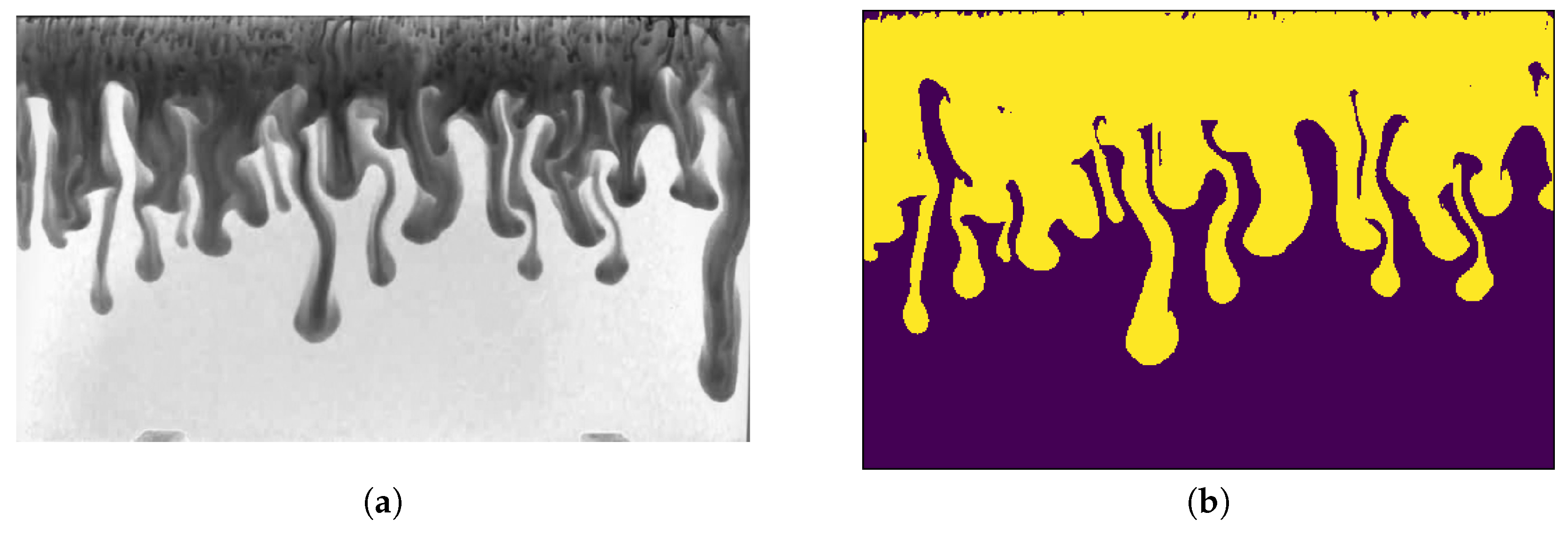
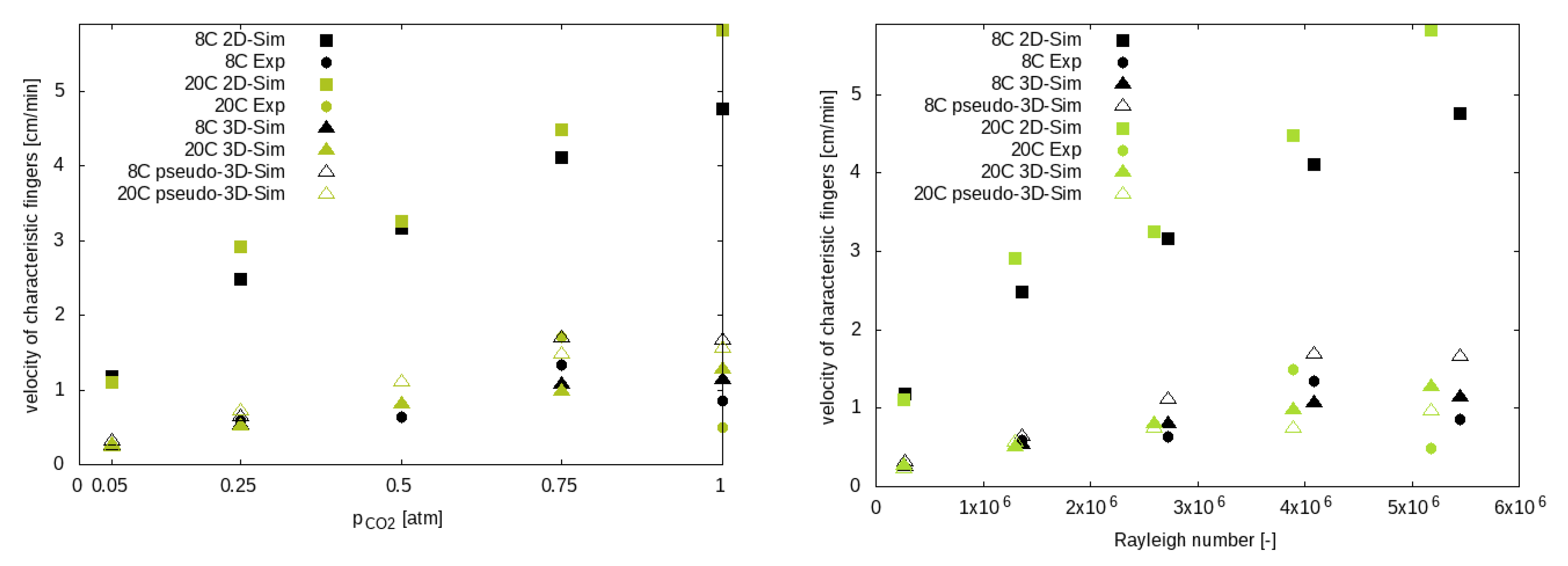
We consider the velocities of the protruding fingers an important criterion in the comparison between experiments and simulations, since they describe the dynamics of such a setup in the long run. The finger velocities were determined from the images, as explained in
Section 2.1; see also
Figure 2. The same approach as with the images from the experiment has been applied to the plots from the simulations. We used a range between 1 × 10
and 3 × 10
for the mole fraction of CO
in water to identify fingers with sufficiently sharp contrasts. We provide the details in
Supplementary Materials to this manuscript. With this procedure, the characteristic velocities were determined; they are plotted in
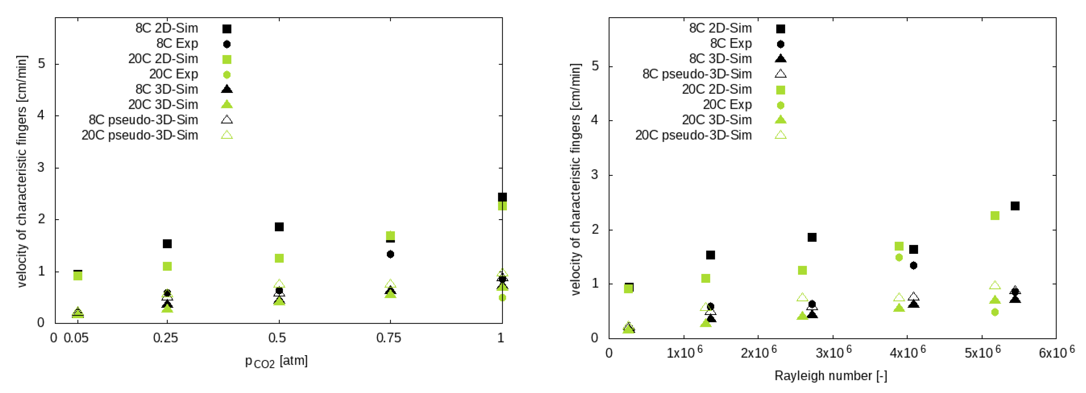
Figure 9 for the graded grid and in
Figure 10 for the regular grid, in both cases depending on the CO
partial pressure and on the Rayleigh number respectively. All plots reveal a tendency towards faster fingers at higher concentrations, and thus higher density differences. Using the same example as for the onset times, i.e., at 8 °C and 0.5 atm, we observed deviations from the experimental value of 393% higher for the 2D graded grid, 25% higher for the 3D graded, 73% higher for the pseudo-3D graded, 33% lower for the 3D regular, 190% higher for the 2D regular, and 11% lower for the pseudo-3D regular. The first obvious observation is that the finger velocities from the 2D model on the graded grid are far from all other data points. This is proof of the importance of considering the wall friction, as we do in the pseudo-3D and in the 3D model. On the regular grid, it is also the 2D finger velocities which have the highest values, but they are much closer to all other data points than on the graded grid. This, in turn, confirms our argument from above that the density difference in the top layers is underestimated on the coarser grid. For the pseudo-3D and the 3D cases, the grid does not have such an obvious effect in the comparison with the experimental data, but with the explanations above, we have clearly made our case for the pseudo-3D model as the best trade-off between desired physical accuracy and computational efficiency.
The “measurement” of fingering velocities is prone to be affected by random effects in the fingering patterns. This might to some extent explain the noise in the data and some outliers we see, for example, at 0.75 and 1 atm, which, however, seem less pronounced in the plot over the Rayleigh number.
Wave lengths were evaluated only qualitatively. They were slightly larger for smaller CO concentrations, as expected, but were not analyzed further.
4. Discussion
The results show a very good agreement between experimental results and numerical simulations on the graded grid, and they were still reasonable on the regular grid. The metrics we used for the comparisons were rather simple and qualitative, but we consider this appropriate given the uncertainties in the experiment. The color indicator has proven useful to visualize the dynamics of the convective fingers, while it compromised the diffusive effects that would counteract the convective growth of the fingers by diluting the concentrations at the finger tips. The qualitative comparison of the density-driven concentration pattern as shown in
Figure 4 and
Figure 5 looks promising, although for later times, the match between experiment and simulation is impaired mainly by the above-mentioned limitations in the experiment. In particular, we note that the shift in onset time and temporal evolution from
Figure 4 to
Figure 5 is in good agreement between experiment and model. The qualitative and quantitative difference in the finger’s dynamics from one scenario to the next is in very good agreement regarding experimental and numerical results. Thus, this study is a significant step towards a successful validation of our Navier–Stokes model with concentration-dependent density.
The 2D simulations neglect the no-slip conditions at the front and back plate of the flume. Thus, as expected, they tend to overestimate the finger growth and propagation velocity, but, as the comparison with the experiment and the 3D simulations shows, this is still within the same order of magnitude. Both the 3D and the pseudo-3D results show a close match in terms of reproducing the characteristic velocity of the fastest fingers; see
Figure 10. Our setup with 1 cm distance between front and back plate is a trade-off between our goals (i) to have the processes in an open water body, and (ii) to use simple imaging by taking a photo of the front glass plate as representative of the fingers developing inside.
Onset times are consistently overestimated in the simulations on the regular grid compared with the experiment. They match well when the graded grid is used, except for the case of a very small CO
concentration being present, where the experimental onset is seen significantly earlier than in all models. The experiment is probably disturbed by non-perfect conditions at the top boundary. The constant gas concentration at the top was achieved not instantaneously, but gradually, according to the velocity of a gas flow along the top of the water body, which was, however, separated from the water by a metal grid to minimize disturbance. Nevertheless, even if small, such a disturbance might lead to a premature triggering of fingers. If so, it does not seem to be very important for a large enough CO
concentration, but for small concentrations where onset is late, it seems to play a role. On the other hand, the buffering by the color indicator should act protractingly. A third point: as we have shown, the implementation of the discretization scheme (see
Section 2.2.2) [
20,
21] can cause a delay of the onset time for coarse grids, since it requires some time to have the first discrete finite volume at the top of the water body at a high enough CO
concentration to trigger instability. While it is not easy to separate these effects quantitatively, we can still state that the agreement between experiment and simulations is very reasonable and the tendency towards longer onset times for lower CO
concentrations is consistently reproduced in all cases.
The influence of temperature is not very distinct and clear. Since the Rayleigh numbers are dependent on the temperature, see
Table 1, the instability at the same CO
concentration should be higher at 8 °C than at 20 °C. Consequently, this would favor an earlier onset and faster fingers at the lower temperature. On the one hand, the density difference is influenced by temperature due to the solubility being temperature-dependent. On the other hand, there is the viscosity as the dampening effect for developing fingers, which shows the opposite tendency. Viscosity is high at low temperatures; thus, the higher instability encounters a more viscous fluid and vice versa. While at 8 °C, the viscosity is higher by a factor of 1.35 than at 20 °C, the density difference at 8 °C is higher by a factor of 1.41 than at 20 °C. Both parameters occur linearly in the numerator and denominator of the Rayleigh number. Therefore, since the relative change is very similar, it is expected that in this case, this has no significant impact on the onset times. Regarding the finger’s velocities, it is not as simple, since the density difference diminishes during the advancement of a finger and viscosity might become the stronger argument. In any case, as we expected, the data from the experiments and models do not give us strong evidence for a temperature dependence.
With respect to the choice of the model, we can state that the 2D model consistently overestimates the dynamics of the fingers, and does so very strongly on the graded grid. While the impact on the onset time is visible, it is much more important for the velocity of the fingers. Shear stress is imposed by the back and front glass plate when fingers start developing. The pseudo-3D model accounts for this with a correction term in the momentum balance. Regarding the metrics we apply, i.e., onset time and velocity of the fingers, the pseudo-3D model achieves very good agreement, since it is close to the results of the full 3D model in all instances. We consider the velocities of the fingers as the most important metric for comparison, and here we clearly see that pseudo-3D and 3D both work well, while the neglection of wall friction in the 2D model is the main reason for the deviations observed.
With regard to the characterization of instability, we tried to use metrics from the abundant literature on the convective dissolution of CO
injected into saline aquifers, where Equations (
9) and (
10) can be used to predict onset time and critical wave length. In our study, we assessed the value of
for the onset time, and found that this proportionality factor is far from being a constant value. Interestingly, when
is divided by the Péclet number as given by Equation (
11), the values obtained are almost constant. This is shown in
Table 3.
While the values for
vary by a factor of about 60 between the respective minimum and maximum values (
Table 2), this variation is reduced to a factor of about 3 for
/Pe (
Table 3). Using the definition of the Pe number from Equation (
11), we can write
From Equation (
15), one can conclude that, with
g,
k, and
all being constant, and
varying only slightly with temperature, an almost constant
/Pe would suggest a rather anti-proportional correlation between
and
. In contrast to that, Equation (
9) suggests that
has a quadratic influence on
.
We note that we did not pursue further theoretical considerations or stability analyses on the given system of equations consisting of Navier–Stokes equation and mass balance equations for the two components coupled via a density depending on concentration. Our study is rather descriptive based on observations, which we have found to be in satisfactory agreement between numerical simulations and experiments.
Finally, let us offer some remarks on the computational efforts in the three different models. We may compare the CPU time required to simulate 2000 s in the case of 8 °C with 50 % CO as the boundary condition using the graded grid. The full 3D model required 152,800 s, the 2D model 525 s, and the pseudo-3D model 325 s. Obviously, the 3D model is by far the most costly. In fact, the pseudo-3D shows the best performance, even in comparison to the 2D model. The tiny additional effort of computing the drag term is easily compensated for in this case by a better convergence of the Newton solver, since velocities in the pseudo-3D are smaller than in the 2D simulations.


